Unsteady Simulation of Transonic Buffet of a Supercritical Airfoil with Shock Control Bump - MDPI
←
→
Page content transcription
If your browser does not render page correctly, please read the page content below
aerospace
Article
Unsteady Simulation of Transonic Buffet of a Supercritical
Airfoil with Shock Control Bump
Yufei Zhang *, Pu Yang, Runze Li and Haixin Chen

                                          School of Aerospace Engineering, Tsinghua University, Beijing 100084, China;
                                          yang-p19@mails.tsinghua.edu.cn (P.Y.); lirz16@mails.tsinghua.edu.cn (R.L.); chenhaixin@tsinghua.edu.cn (H.C.)
                                          * Correspondence: zhangyufei@tsinghua.edu.cn

                                          Abstract: The unsteady flow characteristics of a supercritical OAT15A airfoil with a shock control
                                          bump were numerically studied by a wall-modeled large eddy simulation. The numerical method
                                          was first validated by the buffet and nonbuffet cases of the baseline OAT15A airfoil. Both the pressure
                                          coefficient and velocity fluctuation coincided well with the experimental data. Then, four different
                                          shock control bumps were numerically tested. A bump of height h/c = 0.008 and location xB /c = 0.55
                                          demonstrated a good buffet control effect. The lift-to-drag ratio of the buffet case was increased by
                                          5.9%, and the root mean square of the lift coefficient fluctuation was decreased by 67.6%. Detailed
                                          time-averaged flow quantities and instantaneous flow fields were analyzed to demonstrate the flow
                                          phenomenon of the shock control bumps. The results demonstrate that an appropriate “λ” shockwave
                                          pattern caused by the bump is important for the flow control effect.

                                          Keywords: transonic buffet; large eddy simulation; shock control bump; supercritical airfoil


Citation: Zhang, Y.; Yang, P.; Li, R.;
Chen, H. Unsteady Simulation of           1. Introduction
Transonic Buffet of a Supercritical             Modern civil aircraft usually adopt a supercritical wing and operate at transonic
Airfoil with Shock Control Bump.          speed [1]. Shockwaves appear at both the cruise condition and the buffet condition for
Aerospace 2021, 8, 203.
                                          a supercritical wing or airfoil [2]. The buffet, which is a self-sustained shock oscillation
https://doi.org/10.3390/
                                          induced by periodic interactions between a shockwave and a separated boundary layer [3],
aerospace8080203
                                          is a key constraint of the flight envelope of a civil aircraft [4].
                                                The transonic buffet phenomenon has been studied for decades. It was first observed
Academic Editor: Sergey B. Leonov
                                          by Hilton and Fowler [5] in a wind tunnel investigation. When a buffet occurs, the
                                          shockwave location and the lift coefficient, as well as the turbulent boundary layer thickness
Received: 28 June 2021
Accepted: 22 July 2021
                                          after the shockwave, change periodically [5]. Iovnovich and Raveh [6] classified transonic
Published: 26 July 2021
                                          buffets into two types: one is where a shock oscillation appears on both the upper side
                                          and lower side of the wing, while the other is where an oscillation only exists on the upper
Publisher’s Note: MDPI stays neutral
                                          side. The latter is more common for a supercritical wing of a civil aircraft [7]. Pearcey
with regard to jurisdictional claims in
                                          et al. [8] studied the relation between the flow separation near the trailing edge and the
published maps and institutional affil-   onset of a buffet, which is widely used in the determination of the buffet onset boundary [3].
iations.                                  When the shockwave strength is weak, which is the case for a supercritical airfoil, the
                                          Kutta wave is believed to play an important role in the shockwave oscillation [9,10]. A self-
                                          sustained feedback model of a shockwave buffet was proposed by Lee et al. [10]. The model
                                          illustrated that when the pressure fluctuation of the shockwave propagates downstream of
Copyright: © 2021 by the authors.
                                          the trailing edge, the sudden change in the disturbance forms a Kutta wave propagating
Licensee MDPI, Basel, Switzerland.
                                          upstream, and the shockwave is made to oscillate by the energy contained in the Kutta
This article is an open access article
                                          wave [10]. The Kutta wave, which propagates by the speed of sound [10], is also considered
distributed under the terms and           a sound wave generated at the trailing edge [11]. Chen et al. [12] further extended the
conditions of the Creative Commons        feedback model to more types of shockwave oscillations. Crouch et al. [13] found that
Attribution (CC BY) license (https://     both the stationary mode and oscillatory mode of instability occur on an unswept buffet
creativecommons.org/licenses/by/          wing, and that the intermediate-wavelength mode has a flow feature of the airfoil buffeting
4.0/).                                    mode.

Aerospace 2021, 8, 203. https://doi.org/10.3390/aerospace8080203                                          https://www.mdpi.com/journal/aerospace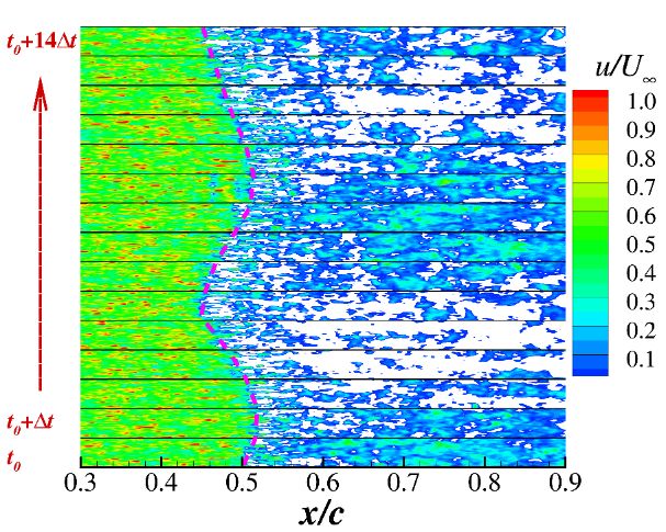
Aerospace 2021, 8, 203                                                                                           2 of 18

                               Experimental [14,15] and numerical investigations [16–18] have been widely used in
                         buffet studies in recent years. The transonic buffet characteristics of an OAT15A supercriti-
                         cal airfoil were experimentally measured [14] and widely adopted as a validation case for
                         numerical study. The unsteady Reynolds-averaged Navier–Stokes (RANS) method [16] and
                         detached eddy simulation [17] can resolve the large-scale pattern of a transonic buffet and
                         determine the main frequency of the shockwave oscillation, while a large eddy simulation
                         (LES) [18] can provide abundant details of the interaction between the shockwave and
                         turbulence structures inside the boundary layer.
                               The buffet onset boundary determines the flight envelope of a civil aircraft [19]. Sup-
                         pressing the shockwave oscillation and improving the buffet onset lift coefficient are vital
                         for modern civil aircraft design. Vortex generators [20] and shock control bumps (SCBs) [21]
                         are two common passive flow control devices used for transonic buffets. The vortex gener-
                         ator has been intensively studied and widely adopted on Boeing’s civil aircraft to control
                         the transonic buffet [22]. However, SCBs are still receiving considerable research attention
                         and are not yet practical on civil aircraft. SCBs can be classified into two-dimensional
                         (2D) bumps and three-dimensional (3D) bumps [23]. The 2D bump is identical along the
                         spanwise direction, while the 3D bump can have different shapes in the spanwise direction.
                               The basic control mechanism of a 2D SCB is a combination of the compression wave
                         and expansion wave near the shockwave [24]. A supercritical airfoil usually has a weak
                         normal shock on the upper surface. If a bump is placed at the shockwave location, a
                         compression wave can be formed when the flow moves upward from the bump and
                         weakens the normal shock. Expansion waves downside of the bump are also beneficial
                         for pressure recovery after the shockwave. With the compression and expansion waves, a
                         “λ” shockwave structure is formed instead of a normal shock on the airfoil [25], meaning
                         the wave drag can be reduced. As the benefit comes from the interaction between the
                         shockwave and the bump, the drag reduction effect is relevant to the bump location and
                         height. Sabater et al. [26] applied a robust optimization on the location and shape of a 2D
                         SCB and achieved a drag reduction of more than 20% on an RAE2822 airfoil. Jia et al. [27]
                         found that a 2D SCB can reduce the drag coefficient at a large lift coefficient; however,
                         it increases the drag coefficient at a small lift coefficient. Adaptive SCBs [28,29], which
                         change shapes according to the shockwave location, provide drag reduction effectiveness
                         under a wide range of flow conditions. Lutz et al. [30] optimized adaptive SCBs and found
                         the drag curve shows significant improvement compared to the initial airfoil.
                               The control mechanism of a 3D SCB includes not only the “λ” shockwave structure
                         formed by the bump but also the vortical flow induced by the bump [31], which is similar
                         to a small vortex generator [32]. The streamwise vortex induced by the edge of the 3D SCB
                         is beneficial for the mixing of high-energy outer flow and low-energy boundary layer flow,
                         consequently suppressing the flow separation. A 3D bump with a wedge shape [33,34] or
                         hill shape [31,35,36] can effectively induce a vortical flow after the bump and change the
                         shockwave behavior.
                               SCBs have shown great potential for buffet control. However, there are also some
                         issues mentioned in the literature. One of the concerns is that the control efficiency is
                         sensitive to the shock location [37]. This might decrease the performance at the off-design
                         condition. An adaptive SCB can extend the effective range of shock control; however, an
                         adaptive SCB might increase the structure complexity and maintenance cost [38].
                               From the numerical method perspective, the steady [39,40] or unsteady [32,41] RANS
                         method has been widely used in the study of buffets or in the shape design of SCBs for
                         supercritical airfoils. However, the control effect of SCBs is rarely studied by high-fidelity
                         turbulence simulation methods such as the RANS–LES hybrid method or the LES method.
                         As stated before, a buffet is a natural unsteady turbulent flow that includes periodic
                         shockwaves and a thickened turbulent boundary layer under a high Reynolds number. A
                         large eddy simulation can resolve the small-scale turbulent structures of the boundary and
                         the generated acoustic waves of the tailing edge [18], which is a superior method to study
                         the unsteady interaction mechanism between the shockwave and the SCB.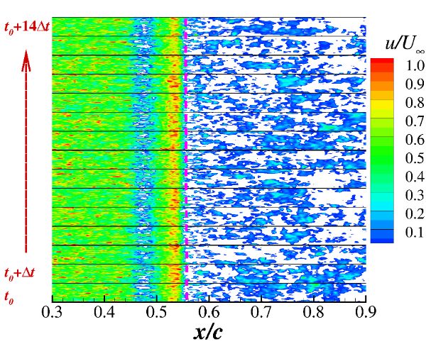
Aerospace 2021, 8, 203                                                                                            3 of 18

                              In this paper, the transonic buffet of an OAT15A supercritical airfoil with an SCB was
                         numerically studied by a wall-modeled large eddy simulation (WMLES). The numerical
                         method was validated by the experimental data of the OAT15A airfoil. Several 2D SCBs
                         were adopted to test the control effect of the unsteady flow. The flow fields of both the
                         nonbuffet case and buffet case were analyzed. To the authors’ knowledge, this is the first
                         study to use a large eddy simulation on the SCB of a supercritical airfoil. The time-averaged
                         flow quantities, periodic flow patterns and pressure fluctuations were compared for the
                         airfoil without or with an SCB.

                         2. Numerical Method and Validation
                         2.1. Numerical Method
                               In this paper, a wall-modeled large eddy simulation was adopted to compute the flow
                         field of an OAT15A supercritical airfoil. The solver was developed based on a finite-volume
                         CFD code [42,43]. The inviscid flux was computed based on a blending of an upwind
                         scheme and a central difference scheme [44,45]. The time advancing method is a three-
                         step Runge–Kutta method. Vreman’s eddy viscosity model [46] was used to model the
                         subgrid-scale turbulence motion. Based on the estimation of Choi and Moin [47], the grid
                         requirement of a wall-resolving large eddy simulation is proportional to Re13/7  L   , and L is
                         the character length of the flow field; in contrast, the grid requirement of a wall-modeled
                         simulation is proportional to Re L . In this study, the computational cost of a wall-resolving
                         LES was too high because the Reynolds number is 3 × 10⁶ . Consequently, an equilibrium
                         stress-balanced equation was solved to model the energy-containing eddies in the inner
                         turbulent boundary layer [44,45]. The wall-modeled equation was solved on an additional
                         one-dimensional grid with 50 grid points to obtain the velocity profile of the inner layer
                         of the boundary layer. The shear stress provided by the wall-modeled equation was
                         applied as the boundary condition of the Navier–Stokes equation. The velocity of the
                         upper boundary of the wall-modeled equation was interpolated from the third layer of
                         the LES grid. The numerical method is not the focus of this paper. Consequently, detailed
                         numerical schemes and formulas are not presented here. Readers can refer to our previous
                         work on high-Reynolds separated flows [44,45].

                         2.2. Computational Grid
                               The computational grid used in this paper was a C-type grid, which was generated
                         by an in-house grid generation code that solves Poisson’s equation. The computational
                         domain was [−18c, 20c] in the x direction and [−20c to 20c] in the y direction (c is the
                         chord length). Although the bump shape was two-dimensional, we carried out a three-
                         dimensional simulation because of the three-dimensional nature of the turbulence. The
                         spanwise length was 0.075c, which is larger than the WMLES in the study by Fukushima
                         et al. [18]. The grid had 1945 points in the circumferential direction and 261 points in the
                         normal direction. It had 51 points evenly located in the spanwise direction. The trailing
                         edge thickness was 0.005c, and a grid block with 21 × 51 × 249 points was located on the
                         trailing edge region. The total grid number was 26.2 million. Figure 1a shows the grid of
                         the x–y plane of the baseline OAT15A airfoil. The figure is plotted by every two points
                         of the grid. Figure 1b shows the wall grid near the leading edge of the airfoil. The first
                         layer height of the grid was 2.0 × 10⁻⁴ c. The increasing ratio in the normal direction was
                         less than 1.1. The first grid layer can be located in the logarithmic layer of the turbulent
                         boundary layer because the wall-modeled equation can provide the shear stress boundary
                         condition of the wall. When the SCB was installed on the airfoil surface, the wall surface
                         was deformed to simulate the effect of the bump while keeping the grid topology and grid
                         number the same.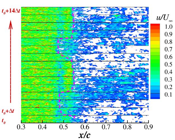
Aerospace
Aerospace 2021, 2021,PEER
8, x FOR 8, x FOR PEER REVIEW
REVIEW 4 of 18 4 of 18
Aerospace 2021, 8, 203 4 of 18
When theWhen
SCB the
wasSCB was installed
installed on thesurface,
on the airfoil airfoil surface,
the wallthe wall was
surface surface was deformed
deformed to sim- to sim-
ulate the effect of the bump while keeping the grid topology and grid number
ulate the effect of the bump while keeping the grid topology and grid number the same. the same.
(a) grid
(a) Surface Surface grid
in the in plane
x–y the x–y plane (b) Wall(b) Wall
grid neargrid
thenear the edge
leading leading edge
Figure 1. Figure 1. Computational
Computational grid
grid of grid
the of the OAT15A
baseline baseline OAT15A airfoil.
airfoil. airfoil.
Figure 1. Computational of the baseline OAT15A
2.3. Validation
2.3. Validation of the Baseline
of the Baseline OAT15AOAT15A Airfoil Airfoil
2.3. Validation of the Baseline OAT15A Airfoil
The baseline The baseline
OAT15AOAT15A airfoil was airfoil
adoptedwas adopted as the validation
as the validation case. Thecase. flowThe flow condition
condition
The baseline OAT15A airfoil 6was adopted as the validation case. The flow condition
was Ma = 0.73 and Re = 63.0 × 10
was Ma = 0.73 and Re = 3.0 × 10 . [14] The6 nondimensional time step was ΔtU∞/c = 1.37∞/c× = 1.37 ×
. [14] The nondimensional time step was ΔtU
was Ma = 0.73
10 . Approximately and Re = 3.0 × 10 . [14] The nondimensional time
(tU∞/c) were computed for each case, and the ∞ step was ∆tU /c 100
=
180 time180 time(tUunits last
−4
10−4. Approximately −4 . Approximately units ∞/c) were computed for each case, and the last 100
1.37
time × 10
units were applied for 180
flow time units (tU
field statistics. /c) were computed for each
∞ It cost approximately5 2.0 × 10⁵ core hours case, and the
time units
last
were
100 time
applied
units
for flow
were
field
applied
statistics.
for flowwith
It cost approximately
field astatistics.
2.0 × 10 core hours
cost approximately 2.0 × 10⁵ core
for each for
floweachcase flow
on case
an on
Intel an Intel
cluster cluster
with a 2.0 GHz 2.0 GHzItCPU.
CPU.
hours The for each+ and flowΔy case+ ofon anfirst
Intel cluster with
werea collected
2.0 GHz CPU.
The ΔxThe + and Δx Δy + of the first the
grid layer grid werelayer
collected to demonstrateto demonstrate
the gridthe the grid resolu-
resolu-
tion of ∆x present
the
+ and ∆ycomputation.
+ of the first grid Figure layer2a were
shows collected
the Δx to demonstrate
+ and Δy + of the LES gridcollected
grid resolu-
tion of tion
the present computation.
of the present computation.FigureFigure2a shows the Δxthe
2a shows
+ and
∆xΔy+ and+ of ∆y
the+LESof thegrid
LES collected
grid collected
by an angleby an angle of attack
= 2.5°.ααΔy = +2.5°. Δy + was approximately 50upper
on thesurface
upper and surface and 80 on
by anof attack
angle of αattack = 2.5 was
◦ ∆y
+ .was
approximately
+ was approximately 50 on the 50 on +the upper surface 80 on and 80
the lower the lower
surface, surface, while Δx approximately twice the Δy . The first grid point in the
lowerwhile Δx while
was approximately twice the Δy . The thefirst
∆y+ grid
. Thepoint in the
+ +
on the surface, ∆x+ was approximately twice first grid point in
wall normalwall normal
direction direction was located at the logarithmic layer of a turbulent boundary layer,
the wall normalwas locatedwas
direction at the logarithmic
located layer of a turbulent
at the logarithmic layer of boundary
a turbulent layer,
boundary
which satisfies
which layer,
satisfies the requirement
the requirement for a WMLES. for a WMLES. Δy+ The Δy of the
+ first grid layer of the wall-
which satisfies the+ requirement forThe
a WMLES. of theThefirst∆y+grid layer
of the firstofgrid
the wall-
layer of the
modeled modeled
equation (Δy equation (Δy
wm) was(∆y
wm)+was always less than 1.0, as shown in Figure 2b. This is suffi-
always) less wasthan 1.0,less
as shown in asFigure 2b.inThis is suffi-
+
wall-modeled equation always than 1.0, shown Figure 2b. This is
cient to describe
cient tosufficient
describe the viscous viscouswm
the sublayer sublayer
of the of the turbulent
turbulent boundary boundary
layer. Thelayer. The spanwise
spanwise cor- cor-
to describe the viscous sublayer of the turbulent boundary layer. The spanwise
relation
relationcorrelation [43]
[43] of the[43] of the
pressure pressure
fluctuation fluctuation
was computed was computed
to test the to test the
spanwise spanwise
domain. domain.
As As
of the pressure fluctuation was computed to test the spanwise domain. As
shownshown shown
in Figure in Figure 3, the
3, the correlations correlations
of bothofx/c of both
= 0.4 x/c = 0.4 and 0.8 damp fast in the spanwise
in Figure 3, the correlations both x/cand= 0.40.8and
damp fast in fast
0.8 damp the inspanwise
the spanwise
direction, direction,
which which demonstrates
demonstrates that the that the spanwise
present present spanwise
domain domain
size (0.075sizec) (0.075
is c) is adequate.
adequate.
direction, which demonstrates that the present spanwise domain size (0.075 c) is adequate.
(a) Δx
(a) Δx+ and Δy+ and
+ ΔyLES
of the of the
gridLES grid
+ (b)the
(b) Δy+ of Δywall-modeled
of the wall-modeled
+
grid grid
2.Figure 2.Δy
+Δx + and Δy+ of the first grid layer and the wall-modeled grid (Ma = 0.73, Re = 3.0 × 10⁶, α = 2.5°).
FigureFigure
Δx+ 2.
and∆x + of
and ∆y
the+first grid
of the layer
first gridand theand
layer wall-modeled grid (Ma
the wall-modeled = 0.73,
grid (Ma = Re0.73,
= 3.0Re
× 106, α×
= 3.0 106 , α = 2.5◦ ).
= 2.5°).
Figure 4 shows the lift and drag coefficient histories at three different angles of attack.
When a buffet does not occur (α = 2.5◦ ), the lift and drag coefficients have oscillations with
small amplitudes. Then, the amplitude of oscillation is increased at α = 3.0◦ . When α = 3.5◦ ,
a clear periodic oscillation pattern appears on both the lift and drag coefficients, which
demonstrates that a buffet occurs.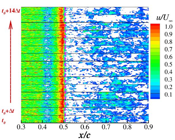
Aerospace2021,
Aerospace 2021,8,8,xxFOR
FORPEER
PEERREVIEW
REVIEW 55of
of18
18
Aerospace 2021, 8, 203 5 of 18
Aerospace 2021, 8, x FOR PEER REVIEW 5 of 18
Figure3.3.Spanwise
Figure Spanwisecorrelation
correlationof
ofthe
thepressure
pressurefluctuations.
fluctuations.
Figure44shows
Figure showsthe thelift
liftand
anddrag
dragcoefficient
coefficienthistories
historiesat
atthree
threedifferent
differentangles
anglesof
ofattack.
attack.
When a buffet does not occur (α = 2.5°), the lift and drag coefficients have oscillations
When a buffet does not occur (α = 2.5°), the lift and drag coefficients have oscillations with with
smallamplitudes.
small amplitudes.Then,
Then,the
theamplitude
amplitudeof ofoscillation
oscillationisisincreased
increasedat atαα==3.0°.
3.0°.When
Whenαα==3.5°,
3.5°,
aa clear
clear periodic
periodic oscillation
oscillation pattern
pattern appears
appears on on both
both the
the lift
lift and
and drag
drag coefficients,
coefficients, which
which
Figure3.3.Spanwise
Figure
demonstratesSpanwise correlation
thatcorrelation ofofthe
thepressure
pressurefluctuations.
fluctuations.
demonstrates that aabuffet
buffetoccurs.
occurs.
Figure 4 shows the lift and drag coefficient histories at three different angles of attack.
When a buffet does not occur (α = 2.5°), the lift and drag coefficients have oscillations with
small amplitudes. Then, the amplitude of oscillation is increased at α = 3.0°. When α = 3.5°,
a clear periodic oscillation pattern appears on both the lift and drag coefficients, which
demonstrates that a buffet occurs.
Figure 4.
Figure Liftand
4. Lift anddrag
dragcoefficient
coefficient histories
histories of
historiesof the
ofthe OAT15A
theOAT15A airfoil.
OAT15Aairfoil.
airfoil.
The
Thelift
The lift coefficient
liftcoefficient
coefficientwaswas time-averaged
wastime-averaged
time-averagedfor for comparison
forcomparison
comparisonwith with
withthethe experimental
theexperimental data,
experimentaldata, as
data,asas
shown
shown in
in Figure
Figure 5.
5. The experimental
The experimental datadata were
were extracted
extracted from
from [48].
[48]. There
There were
were two
two series
series
shown in Figure 5. The experimental data were extracted from [48]. There were two series
of experimental
ofexperimental
experimentaldata data
datainin the
inthe reference.
thereference. One
reference.One
Onewaswas from
wasfrom
fromthethe S3MA
theS3MA
S3MAwind wind tunnel,
windtunnel, and
tunnel,and the
andthe other
theother
other
of 6
was from
was from
from the the T2
the T2 wind
T2 wind tunnel.
wind tunnel. The
tunnel. The Reynolds
The Reynolds number
Reynolds number
number in in that
in that experiment
that experiment was
experiment was 6.0
was 6.0 × 10
1066,,,
6.0 ×× 10
was
Figureis
which
which 4.higher
Lift andthan
dragthecoefficient
presenthistories
present of the OAT15A
computation. Although airfoil.
the flow condition was slightly
which isis higher
higher than
than the
the present computation.
computation. Although
Although the flow
the flow condition
condition was
was slightly
slightly
different
different from
from the
the present
present computation,
computation, the
the time-averaged
time-averaged lift
lift coefficients
coefficients of
of the
the present
present
different from the present computation, the time-averaged lift coefficients of the present
The lift were
computation coefficient
locatedwas time-averaged
between the two for comparison
series of with the
experimental data.experimental data, as
computation were located between the two series of experimental
computation were located between the two series of experimental data. data.
shown in Figure 5. The experimental data were extracted from [48]. There were two series
of experimental data in the reference. One was from the S3MA wind tunnel, and the other
was from the T2 wind tunnel. The Reynolds number in that experiment was 6.0 × 10⁶,
which is higher than the present computation. Although the flow condition was slightly
different from the present computation, the time-averaged lift coefficients of the present
computation were located between the two series of experimental data.
Figure5.
Figure
Figure 5.Comparison
5. Comparisonof
Comparison ofthe
of thecomputed
the computedlift
computed liftcoefficient
lift coefficientwith
coefficient withexperimental
with experimentaldata
experimental data[48].
data [48].
[48].
The mean
The mean pressure
pressure coefficient
coefficient was
wascompared
was compared with
compared with the
with the experimental
the experimental data
experimental data of
data of [14].
[14]. As
As
As
shown in Figure 6, the pressure coefficients at
coefficients at
shown in Figure 6, the pressure coefficients three
at three different
three different angles
different angles
angles ofof attack
of attack coincide
attack coincide well
coincide well
well
withthe
with theexperimental
experimentaldata,
data,except
exceptthat
thatthe
theshockwave
shockwavelocation
locationisisslightly
slightlydownstream
downstreamof
downstream of
of
the experimental
the experimental data.
data.
Figure 5. Comparison of the computed lift coefficient with experimental data [48].
The mean pressure coefficient was compared with the experimental data of [14]. As
shown in Figure 6, the pressure coefficients at three different angles of attack coincide well
with the experimental data, except that the shockwave location is slightly downstream of
the experimental data.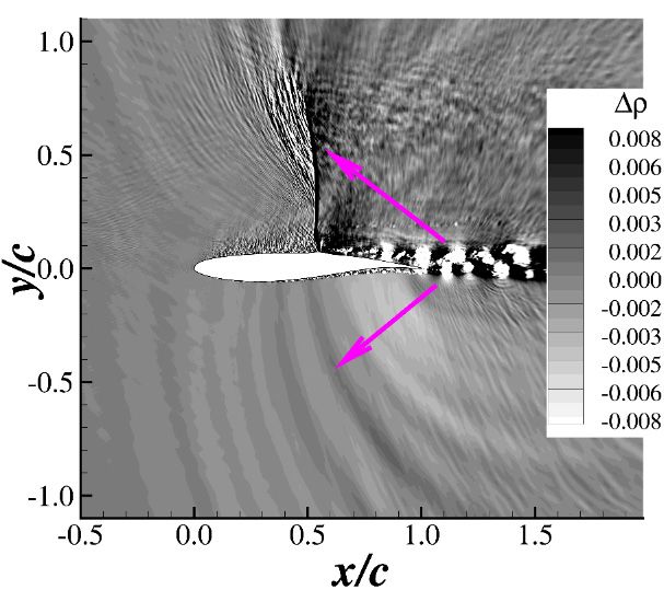
Aerospace 2021, 8, x FOR PEER REVIEW 6 of 18
x FOR PEER REVIEW
Aerospace 2021, 8, 203 6 of 18
(a) α = 2.5° (b) α = 3.0°
(a) α = 2.5° (b) α = 3.0°
(c) α = 3.5°
(c) α = 3.5°
Figure 6. Comparison of pressure coefficients at different angles of attack (Ma = 0.73, Re = 3.0 × 10⁶).
Figure6.
Figure 6. Comparison
Comparison of
of pressure
pressurecoefficients
coefficientsat
atdifferent
differentangles
anglesof
ofattack
attack(Ma
(Ma==0.73,
0.73,Re
Re== 3.0
3.0 ×
× 10
106).).
6
Figure 7a shows the mean Mach contour at α = 3.5°.◦ It is clear that a low-speed region
Figure
Figure 7a shows the mean Mach contour contour at αα = 3.5°.
3.5 . It
It is
is clear
clear that
that aa low-speed
low-speed region
appears near the trailing edge of the airfoil. The mean shockwave is also smeared because
appears
appears near the trailing edge of the airfoil. The mean shockwave
The mean shockwave is also smeared because
of the periodic oscillation of the shock location. Figure 7b demonstrates the root mean
of
of the periodic oscillation of the shock location. Figure Figure 7b demonstrates
demonstrates the root mean
square (RMS) of the pressure fluctuations. It is normalized by the dynamic pressure of the
square
square (RMS)
(RMS)of ofthe
thepressure
pressurefluctuations.
fluctuations.It It
is normalized
is normalized by by thethe
dynamic
dynamic pressure of the
pressure of
freestream condition. The maximum pressure fluctuation appears near the shockwave lo-
freestream condition.
the freestream condition.TheThe
maximum
maximum pressure
pressurefluctuation appears
fluctuation appearsnearnear
the the
shockwave
shockwavelo-
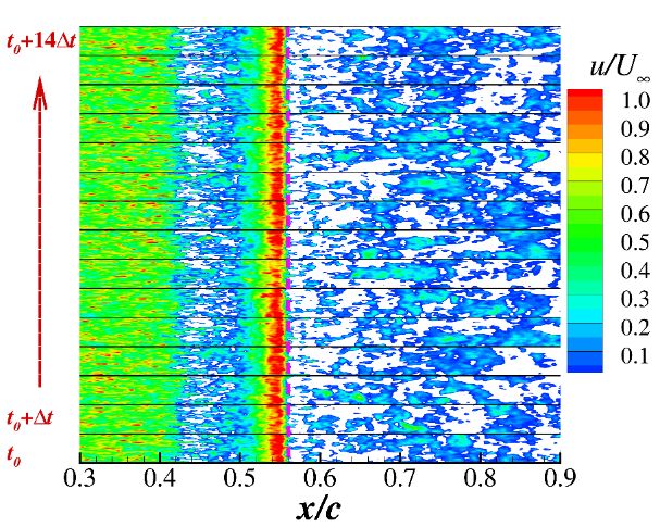
cation. Figure 8 compares the RMS of the streamwise velocity fluctuation with the exper-
cation. Figure
location. 8 compares
Figure 8 comparesthe RMS of theofstreamwise
the RMS velocity
the streamwise fluctuation
velocity with the
fluctuation exper-
with the
imental data of the S3Ch wind tunnel [49]. The values in Figure 8 are dimensional, and
experimental
imental data
data of theof the S3Ch
S3Ch wind wind
tunneltunnel [49].values
[49]. The The values
in Figurein Figure
8 are8dimensional,
are dimensional,
and
the contours have the same legend. The contours of the computation and experiment are
andcontours
the the contours
havehave the same
the same legend.
legend. The The contours
contours of computation
of the the computation andand experiment
experiment are
quite consistent in both shape and value, which validates that the present computational
are quite
quite consistent
consistent in both
in both shape
shape andand value,
value, whichvalidates
which validatesthat
thatthethepresent
present computational
computational
method
methodisisreliable.
method reliable.
(a) Mach contour (b) RMS of pressure fluctuation
(a) Mach contour (b) RMS of pressure fluctuation
Figure 7. Mean flow field and pressure fluctuations
fluctuations (Ma =
= 0.73, Re
Re = 3.0 ××10
10,66,α
6
, αα===3.5°).
3.5◦ ).
Figure7.7.Mean
Figure Meanflow
flowfield
fieldand
andpressure
pressure fluctuations(Ma
(Ma =0.73,
0.73, Re==3.0
3.0 × 10 3.5°).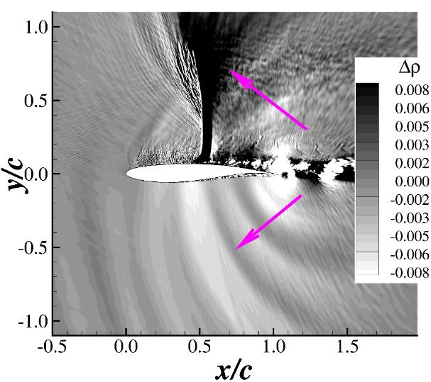
Aerospace 2021, 8, x FOR PEER REVIEW 7 of 18
Aerospace 2021,
Aerospace 2021, 8,
8, 203
x FOR PEER REVIEW of 18
7 of 18
(a) (b)
(a) (b)
Figure 8. Comparison of streamwise velocity fluctuation (Ma = 0.73, Re = 3.0 × 10⁶, α = 3.5°). (a) Experimental data (taken
Figure 8. Comparison
Comparison
from [49]),
Figure 8. of
(b) presentof streamwisevelocity
computation.
streamwise velocityfluctuation
fluctuation(Ma
(Ma==0.73,
0.73,Re
Re==3.0
3.0×× 10
1066,, α
α== 3.5°).
3.5◦ ). (a)
(a) Experimental data (taken
Experimental data (taken
from [49]), (b) present computation.
from [49]), (b) present computation.
Figure 9 further compares the wall pressure fluctuation at α = 3.5°. The experimental
◦ . The experimental
data Figure 9 further from
were extracted compares
[14]. the wall
Thewall pressure
pressure
computed fluctuation
fluctuation
location atpeak
at
of the αα== 3.5
3.5°.
fluctuation is slightly
data were extracted from [14]. The computed location of the peak
downstream, which is consistent with the pressure coefficient distribution (Figurefluctuation is slightly
slightly
6c).
downstream, which
which is consistent
consistent with
with the pressure coefficient distribution
However, the peak value of the present computation is close to the experiment, which (Figure 6c).
However,
means thatthethepeak valueshock
primary of the present
present
buffet computation
computation
phenomenon is close
is wellclose to the
to
captured theby experiment,
experiment, which
which
the computation.
means that the primary
The motivation shock buffet
of the present paper phenomenon
was to study is thewell captured
effect by thecontrol
of the shock computation.
bump.
The motivation
The motivation ofthe
of
variation causedthepresent
bypresent paper
the paper
bump, was
was to to
rather study
study
than thethe
the effect
effect of
of the
accurate the
shock
shockwave shock control
control bump.
location, bump.
is The
our
variation
The caused
variation by
causedthebybump,
the rather
bump, than
ratherthe accurate
than the shockwave
accurate location,
shockwave
focus in the following sections. Consequently, the numerical method is validated to be is our
location,focus
is in
our
the following
focus in the
practicable. sections.
following Consequently,
sections. the numerical
Consequently, the method
numerical is validated
method isto be practicable.
validated to be
practicable.
Figure 9.
Figure 9. Comparison
Comparison of
of wall
wall pressure
pressure fluctuation
fluctuation (Ma
(Ma == 0.73,
0.73, Re
Re =
= 3.0
3.0 ××10
10,6 ,αα==3.5°).
6
3.5◦ ).
Figure 9. Comparison of wall pressure fluctuation (Ma = 0.73, Re = 3.0 × 10⁶, α = 3.5°).
3. Numerical Study of Shock Control Bump
3. Numerical
3.1. Study of Shock Control Bump
3.1. Shape
Shape of of the
the Shock
Shock Control
Control Bump
Bump
3.1. Shape
In of the Shock Control Bump
In this
this section,
section, aa two-dimensional
two-dimensional SCB SCB is is numerically
numerically tested
tested and and compared
compared with with thethe
baseline
In this
baseline configuration.
configuration. Several bumps
section, a two-dimensional
Several bumps with with is
SCB different heights
numerically
different heights and
tested
andand locations
compared
locations are
are analyzed.
with the
analyzed.
The
The geometries
baseline of
of the
configuration.
geometries the bumps
Severalare
bumps controlled
bumps
are by
by the
with different
controlled the Hicks–Henne
heights andfunction
Hicks–Henne locations[27],
function are as
[27], as shown
analyzed.
shown
in
TheEquation (1). The bump function f (x ) is superposed on
in Equation (1). The bump function f(xB) is superposed on the baseline airfoil. h/cshown
geometries of the bumps are controlled
B by the Hicks–Hennethe baseline
functionairfoil.
[27], h/c
as is
is the
the
relative
in Equation height of
(1). the
The bump,
bump x /c is
function the central
f(x ) is location
superposed andonl is
the
relative height of the bump, BxB/c is the central location andB lB is the bump length. Figure
B the bump
baseline length.
airfoil. Figure
h/c is 10
the
shows
relative
10 shows the geometries
height of
of the bump,
the geometries bumps with
xB/c is with
of bumps different
the central
differentparameters.
location Four
and lB is
parameters. bumps
the bumps
Four are computed
bump length. Figure
are computed in
this
10 paper,
in shows
this paper, as shown
the geometries in
as shown in Figure 10a.
of Figure
bumps10a. The lengths
withThe differentof
lengths the bumps
parameters. are
of the bumps 0.2c.
Fourare The
bumpsfirst three bumps
are computed
0.2c. The first three
are
in this located
paper, at
as x
bumps are all located at xB/c = 0.55, which is the shockwave location of theOAT15A
all shown
B /c = 0.55,
in which
Figure 10a.is the
The shockwave
lengths of location
the bumps of the
are baseline
0.2c. The first three
baseline
airfoil.
bumps The
are relative
all locatedheights
at x h/c
/c = of the
0.55, first
which three
is bumps
the are
shockwave 0.004,
OAT15A airfoil. The relative heights h/c of the first three bumps are 0.004, 0.008 and 0.012.
B 0.008
location and
of 0.012.
the The
baseline
fourth bump
OAT15A is located
airfoil. The slightly
relative upstream
heights h/c of xthe
B /cfirst
= 0.50 andbumps
three has the are same height
0.004, 0.008 as
andBump
0.012. 2.
The fourth bump is located slightly upstream xB/c = 0.50 and has the same height as Bump
Figure
The 10b
fourth10b shows
bump the geometries
is located of the
slightly upstream airfoil superposed
xB/csuperposed with
= 0.50 and has the bumps.
thethesame height as Bump
2. Figure shows the geometries of the airfoil with bumps.
2. Figure 10b shows the geometries of the airfoil superposed with the bumps.
h π ( x/c − x B /c) π
f ( x B ) = · sin4 + , x B /c − l B /2 ≤ x/c ≤ x B /c + l B /2 (1)
c lB 2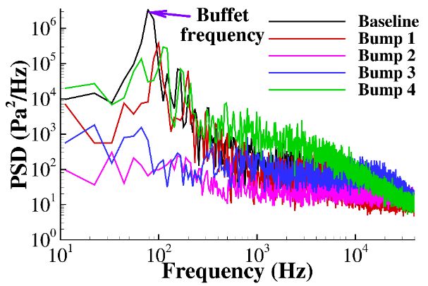
h π ( x c − xB c) π
f ( xB ) = ⋅ sin 4 + , xB c − lB 2 ≤ x c ≤ xB c + lB 2 (1)
c lB 2
The computational settings are the same as the baseline OAT15A airfoil in Section 2.
Aerospace 2021, 8, 203 8 of 18
The computational grids of the bump configurations are deformed from the baseline grid,
which keeps the computation appropriate to compare with the baseline OAT15A airfoil.
(a) Shapes of four different bumps (b) Geometries of the airfoil superposed with bumps
Figure
Figure10.
10.The
Thegeometries
geometriesof
ofthe
theshock
shockcontrol
controlbumps.
bumps.
The computational
3.2. Time-Averaged settingsofare
Characteristics thethe same
Airfoil as the
with baseline OAT15A airfoil in Section 2.
Bumps
The The
computational grids of the bump configurations
aerodynamic performance of the airfoil with arebumps
deformed
wasfrom the baseline
computed grid,
and com-
which keeps the computation appropriate to compare with the baseline OAT15A airfoil.
pared with the baseline airfoil. The nondimensional time step is ΔtU∞/c = 1.37 × 10 . The
−4
flow field of the baseline
3.2. Time-Averaged airfoil isofused
Characteristics as thewith
the Airfoil initial
Bumpscondition of the bump cases. More
than 130 time units (tU∞/c) are computed for each case. The last 80 time units are used for
The aerodynamic performance of the airfoil with bumps was computed and compared
time averaging to obtain the aerodynamic coefficients. Six cases were computed, which
with the baseline airfoil. The nondimensional time step is ∆tU∞ /c = 1.37 × 10⁻⁴ . The flow
are α = 3.5° for all four bumps and α = 2.5° for Bump 2 and Bump 4.
field of the baseline airfoil is used as the initial condition of the bump cases. More than
Figure 11 shows the histories of the lift and drag coefficients in the computation. It is
130 time units (tU∞ /c) are computed for each case. The last 80 time units are used for time
obvious that the periodic oscillation of the lift and drag coefficients at α = 3.5° is sup-
averaging to obtain the aerodynamic coefficients. Six cases were computed, which are
pressed◦by Bumps 2, 3 and 4, while Bump 1 has very little effect on the lift oscillation. It
α = 3.5 for all four bumps and α = 2.5◦ for Bump 2 and Bump 4.
can be seen that the bumps may have a negative influence on the lift coefficient. The lift
Figure 11 shows the histories of the lift and drag coefficients in the computation. It is
coefficient is more or less decreased at α = 3.5°, while it is significantly decreased at the
obvious that the periodic oscillation of the lift and drag coefficients at α = 3.5◦ is suppressed
nonbuffet condition α = 2.5°. Moreover, the drag coefficient is also influenced by the
by Bumps 2, 3 and 4, while Bump 1 has very little effect on the lift oscillation. It can be seen
bumps. The drag coefficient at α = 2.5° is notably increased, as shown in Figure 11d.
that the bumps may have a negative influence on the lift coefficient. The lift coefficient
The or
is more time-averaged
less decreased values
at α = of3.5
the◦ , aerodynamic coefficientsdecreased
while it is significantly are listed at intheTable 1. The
nonbuffet
relative variations ◦(in percentage) in the coefficients compared
condition α = 2.5 . Moreover, the drag coefficient is also influenced by the bumps. Thewith the baseline configu-
ration are also listed
drag coefficient at α in the◦ parentheses
= 2.5 of the table.
is notably increased, A tendency
as shown in Figure of the
11d.bumps is that the
lift coefficient is consistently decreased by the four bumps
The time-averaged values of the aerodynamic coefficients are listed at both α = 2.5°inandTableα =1.3.5°.
The
The lift coefficient at α = 2.5° is decreased by approximately 5%,
relative variations (in percentage) in the coefficients compared with the baseline configu- and it is decreased by
approximately
ration are also 1% to 5%
listed at αparentheses
in the = 3.5°. Withof increasing
the table.bump height of
A tendency (Bumps
the bumps 1, 2 and 3), the
is that the
lift drop becomes increasingly significant. If the location of the bump
lift coefficient is consistently decreased by the four bumps at both α = 2.5 and α = 3.5◦ . is moved ◦ upstream
(Bumps
The lift 2coefficient
and 4), theatliftα= decrement caused by
2.5◦ is decreased bythe bump becomes
approximately 5%,larger.
and itThe influence of
is decreased by
the
approximately 1% to 5% at α = 3.5 . With increasing bump height (Bumps 1, 2and
bump on the drag coefficient is
◦ distinctly different under the nonbuffet and buffet
3), the
conditions. The drag
lift drop becomes coefficientsignificant.
increasingly is increasedIfatthe α =location
2.5°, andof it
theis bump
reduced at α = 3.5°.
is moved Con-
upstream
sequently,
(Bumps 2 the andlift-to-drag
4), the lift ratio is increased
decrement caused at the buffet
by the casebecomes
bump α = 3.5°, except
larger.for Thetheinfluence
highest
bump
of the (Bump
bump on 3),the
while
drag the lift-to-drag
coefficient ratio is decreased
is distinctly at the nonbuffet
different under the nonbuffet caseand
α =buffet
2.5°.
Consequently,
conditions. The thedrag
bump is beneficial
coefficient for the buffet
is increased 2.5◦and
at α =case , andmight be harmful
it is reduced at αfor the◦ .
= 3.5
nonbuffet case, which coincides with our previous study based
Consequently, the lift-to-drag ratio is increased at the buffet case α = 3.5 , except for theon ◦
Reynolds-averaged
Navier–Stokes
highest bumpcomputation
(Bump 3), while [27]. the
Thelift-to-drag
pitching momentratio isisdecreased
also listedat inthe
the nonbuffet
table. The case
ref-
erence ◦
α = 2.5points of the moment
. Consequently, the bumpare x/c = 0.25 andfory the
is beneficial = 0.buffet
The negative
case andvalue mightmeans a nose-
be harmful for
down moment.case,
the nonbuffet It can be seen
which that thewith
coincides absolute values of
our previous the moment
study based onare all decreased by
Reynolds-averaged
the SCBs; however,
Navier–Stokes the variations
computation [27].are The notpitching
significant.
moment is also listed in the table. The
reference points of the moment are x/c = 0.25 and y = 0. The negative value means a
nose-down moment. It can be seen that the absolute values of the moment are all decreased
by the SCBs; however, the variations are not significant.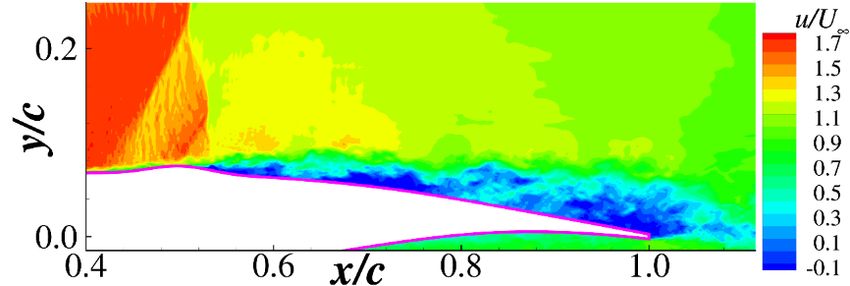
Aerospace 2021, 8, x FOR PEER REVIEW 9 of 18
Aerospace 2021, 8, 203 9 of 18
(a) Lift coefficient at α = 3.5° (b) Drag coefficient at α = 3.5°
(c) Lift coefficient at α = 2.5° (d) Drag coefficient at α = 2.5°
Figure 11. Lift and drag coefficients of the baseline airfoil and airfoil with bumps.
Figure 11. Lift and drag coefficients of the baseline airfoil and airfoil with bumps.
A more interesting phenomenon shown in Table 1 is that regardless of whether the
Table Time-averaged
lift1.and aerodynamic
drag are increased coefficientsthe
or decreased, of the airfoil
RMSs of with bumps.
the coefficients are all suppressed by
the bumps. With increasing bump height, the suppression effect of the lift oscillation is
RMS of
Angle of more significant.
Lift In theofpresent
RMS Lift computation,
Drag Bump 2 has the Lift-to-Drag
highest increment of L/D α
Pitching
Configuration Drag
Attack Coefficient
= 3.5° and a good Coefficient Coefficient
suppression effect on the shockwave Ratio
oscillation. The L/D Moment
of the buffet
Coefficient
case is increased by 5.9%, and the RMS of the lift coefficient fluctuation is decreased by
Baseline 2.5◦ 0.919 0.006884 0.03009 0.000724 30.54 −0.1335
67.6%; consequently, it is considered a good SCB design, with an appropriate height and
airfoil 3.5◦ 0.968 0.037572 0.04823 0.003737 20.07 −0.1262
location.
Bump 1
0.965 0.027828 0.04634 0.003107 20.82 −0.1252
(h/c = 0.004, 3.5◦ Table 1. Time-averaged aerodynamic coefficients of the airfoil with bumps.
(−0.3%) (−25.9%) (−3.9%) (−16.8%) (+3.7%) (+0.8%)
xB /c = 0.55)
Angle of Lift Coeffi- RMS of Lift Drag Coeffi- RMS of Drag Lift-to- Pitching
Configuration 0.866 0.004527 0.03174 0.000662 27.28 −0.1260
Bump 2 2.5◦ Attack
(h/c = 0.008, (−5.8%)cient Coefficient (+5.5%)
(−34.2%) cient Coefficient
(−8.6%) Drag
(−10.6%) Ratio Moment
(+5.6%)
xBBaseline
/c = 0.55) airfoil 2.5° 0.919 0.006884 0.03009 0.000724 30.54 −0.1335
0.953 0.012188 0.04484 0.001569 21.25 −0.1229
3.5◦ 3.5° (−1.5%)0.968 0.037572 0.04823 0.003737 20.07 −0.1262
(−67.6%) (−7.0%) (−58.0%) (+5.9%) (+2.6%)
BumpBump
3 1 0.965 0.027828 0.04634 0.003107 20.82 −0.1252
3.5° 0.917(−0.3%) 0.008297 −(+0.8%)
(h/c = 0.004, x
(h/c = 0.012, B/c 3.5◦
= 0.55) (−25.9%) 0.04642 (−3.9%) 0.001343
(−16.8%) 19.75
(+3.7%) 0.1184
(−5.3%) (−77.9%) (−3.8%) (−64.1%) (−1.6%) (+6.2%)
xB /c = 0.55) 0.866 0.004527 0.03174 0.000662 27.28 −0.1260
2.5°
Bump 2 0.870(−5.8%) 0.003852(−34.2%) 0.03395 (+5.5%) 0.000549
(−8.6%) (−10.6%)
25.63 −(+5.6%)
0.1271
Bump 4 2.5◦
(h/c
(h/c= =
0.008,
0.008,xB/c = 0.55) (−5.3%)0.953 (−44.0%) 0.012188 (+12.8%)0.04484 ( − 24.2%)
0.001569 ( − 16.1%)
21.25 (+4.8%)
−0.1229
3.5°
xB /c = 0.50) 0.925(−1.5%) 0.016171(−67.6%) 0.04559 (−7.0%) 0.002168
(−58.0%) (+5.9%)
20.29 −(+2.6%)
0.1193
3.5◦
Bump 3 (−4.4%)0.917 (−56.9%) 0.008297 ( − 5.5%)
0.04642 ( − 42.0%)
0.001343 (+1.1%)
19.75 (+5.5%)
−0.1184
3.5°
(h/c = 0.012, xB/c = 0.55) (−5.3%) (−77.9%) (−3.8%) (−64.1%) (−1.6%) (+6.2%)
A more interesting phenomenon shown in Table 1 is that regardless of whether the lift
0.870 0.003852 0.03395 0.000549 25.63 −0.1271
and drag are increased or decreased, the RMSs of the coefficients are all suppressed by the
2.5°
Bump 4 (−5.3%) (−44.0%) (+12.8%) (−24.2%) (−16.1%) (+4.8%)
bumps. With increasing bump height, the suppression effect of the lift oscillation is more
(h/c = 0.008, xB/c = 0.50) 0.925 0.016171 0.04559 0.002168 20.29
significant. In the present computation, Bump 2 has the highest increment of L/D −0.1193
α = 3.5◦
3.5°
and a good(−4.4%)
suppression (−56.9%)
effect on the (−5.5%) (−42.0%) The L/D
shockwave oscillation. (+1.1%) (+5.5%)
of the buffet case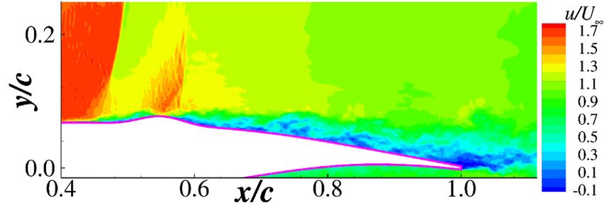
Aerospace 2021, 8, 203 10 of 18
Aerospace 2021, 8, x FOR PEER REVIEW 10 of 18
Aerospace 2021, 8, x FOR PEER REVIEW 10 of 18
is increased by 5.9%, and the RMS of the lift coefficient fluctuation is decreased by 67.6%;
Figure 12 it
consequently, shows the time-averaged
is considered a good SCB Mach contour
design, with ofanthe four bumps.
appropriate Bump
height and1location.
has the
lowest Figure 12 shows the time-averaged Mach contour of the four bumps. Bump 1 hasFigure
height,
Figure 12meaning
shows the
the shock pattern
time-averaged is similar
Mach to the
contour baseline
of the fourconfiguration
bumps. in
Bump 1 has
the
7a.
the A clear “λ”-type shock is formed near the shockwave foot of Bump
lowest height, meaning the shock pattern is similar to the baseline configuration in Figure in
lowest height, meaning the shock pattern is similar to the baseline 2 and Bump
configuration 4.
However,
Figure 7a. the
A “λ”
clear shock of
“λ”-type Bump
shock 4 is
is stronger
formed than
near that
the of Bump
shockwave
7a. A clear “λ”-type shock is formed near the shockwave foot of Bump 2 and Bump 4. 2, which
foot results
of Bump in more
2 and
Bump
lift loss 4.
However,andHowever,
less drag
the “λ” the “λ”
of shock
reduction.
shock Bump of
4 isBump
Bump 3 has4 the
stronger is than
stronger
highest than
bump
that of Bumpthat2,ofwhich
height.Bump 2, which
As results
shown results
inmore
in Figure
inlift
12c, more
the lift
andloss
lossbump and
pushes
less dragless
thedrag
firstreduction.
reduction. shock
BumpupstreamBump
3 has 3and
hasforms
the highest the highest
bump a secondbump
height. height.
shock
As shown As
on in
the shown
bump;
Figure
in12c,
Figure
the 12c,
consequently, bump thepushes
bump pushes
aerodynamic
the the first
first performance
shock shockofupstream
upstream this
and bump
forms and
is forms than
worse
a second ashock
second
the shock
onothers. on the
the bump;
bump; consequently,
consequently, the aerodynamic
the aerodynamic performance
performance of this of this is
bump bump
worse isthan
worse thethan the others.
others.
(a) Bump 1 (b) Bump 2
(a) Bump 1 (b) Bump 2
(c)(c) Bump
Bump 33 (d)
(d) Bump
Bump44
Figure
Figure 12.12. Time-averaged
Time-averaged Machcontour
Mach contourofofthe
thefour
fourbumps
bumps (Ma
(Ma =
= 0.73, Re
0.73, Re
Re===3.0
3.0××
×10
6,6 α = 3.5°).
10
Figure 12. Time-averaged Mach contour of the four bumps (Ma = 0.73, 3.0 106, ,αα==3.5°).
3.5◦ ).
Figure 13presents
Figure presents thepressure
pressure coefficients of the airfoil with bumps. For the drag
Figure 1313 presents the the pressure coefficients
coefficients of
of the
the airfoil
airfoil with
with bumps.
bumps. For For thethe drag
drag
reduction
reduction cases
cases (α(α= = 3.5°),
◦
3.5°), the
the strong
strong shockwave
shockwave of
of the
the baseline
baseline configuration
configuration is divided
is divided
reduction cases (α = 3.5 ), the strong shockwave of the baseline configuration is divided into
into two weak shockwaves. In contrast, for the drag increment cases (α = ◦2.5°), the shock-
into
two two
weak weak shockwaves.
shockwaves. In contrast,
In contrast, fordrag
for the the drag increment
increment casescases
(α = (α
2.5= ),2.5°), the shock-
the shockwave
wave is also divided, but the strength of the second shockwave is even stronger than that
wave
is alsoisdivided,
also divided,
but the but the strength
strength of theof the second
second shockwave
shockwave is evenis stronger
even stronger thanofthat
than that the
of the baseline airfoil.
of the baseline
baseline airfoil.airfoil.
(a) α = 3.5° (b) α = 2.5°
Figure (a) α = 3.5° pressure coefficients for the airfoil with bumps(b) α == 0.73,
2.5° = 3.0 × 10⁶). 6
Figure 13. 13. Time-averaged
Time-averaged (Ma
pressure coefficients for the airfoil with bumps (Ma = 0.73, Re
Re = 3.0 × 10 ).
Figure 13. Time-averaged pressure coefficients for the airfoil with bumps (Ma = 0.73, Re = 3.0 × 10⁶).Aerospace 2021, 8, 203 11 of 18
Aerospace 2021, 8, x FOR PEER REVIEW 11 of 18
Figure 14 shows the time-averaged wall friction coefficient of the airfoil. It is worth
Figure
noting that the14wall
shows the time-averaged
friction is computed bywall the friction coefficient
wall-modeled of theThe
equation. airfoil.
lower It is worth
Aerospace 2021, 8, x FOR PEER REVIEW 11 of 18surface
is hardly influenced by the upper surface bumps, meaning only the lower surface cf surface
noting that the wall friction is computed by the wall-modeled equation. The lower of the
is hardlyairfoil
baseline influenced by the
is plotted upper
in the surface
figure. Thebumps, meaning
wall friction only the
coefficient oflower surface
the upper cf of the
surface is
baselineaffected
strongly airfoil isbyplotted
the in theThe
bumps. figure. Thefirst
friction walldeclines
frictionwhen
coefficient of the upper
approaching the bumpsurfaceand is
Figure 14 shows the time-averaged wall friction coefficient of the airfoil. It is worth
strongly
then
noting
affected
increases
that theonwallbyfriction
the the bumps.
bump, iswhich
The
computed
friction
coincides first
by the with
declines
the tendency
wall-modeled
when approaching
of the
equation. Theflow
the bump
acceleration
lower surface on
and then
theisbump increases
hardly(Figure
influenced on the bump, which coincides with the tendency of the
12).by the upper surface bumps, meaning only the lower surface cf of the flow accelera-
tion on the
baseline bump
airfoil (Figure
is plotted in12).
the figure. The wall friction coefficient of the upper surface is
strongly affected by the bumps. The friction first declines when approaching the bump
and then increases on the bump, which coincides with the tendency of the flow accelera-
tion on the bump (Figure 12).
Figure14.
Figure 14. Wall
Wall friction
frictioncoefficient
coefficientofof
thethe
baseline airfoil
baseline and and
airfoil airfoil with with
airfoil bumps (Ma = (Ma
bumps 0.73, =Re0.73,
= 3.0
× 106, α = 3.5°).6 ◦
Re = 3.0 × 10 , α = 3.5 ).
Figure 14. Wall friction coefficient of the baseline airfoil and airfoil with bumps (Ma = 0.73, Re = 3.0
× 106Figure
, α = 3.5°).15 presents the velocity profile and Reynolds stresses inside the shock-
Figure 15 presents the velocity profile and Reynolds stresses inside the shockwave/boundary
wave/boundary
layer-induced layer-induced flow separation region. Two
at x/c locations at x/c = 0.6 and 0.8
Figure 15flow separation
presents region.
the velocity Two and
profile locations
Reynolds = 0.6 inside
stresses and 0.8 theare presented.
shock-
are
The presented. The velocity
velocity near layer-induced
wave/boundary near
the bump (x/cflow the
= 0.6) bump (x/c
is decreased
separation = 0.6)
region.byTwois decreased
thelocations
bumps, as by the
shown
at x/c bumps,
= 0.6 inand as
Figureshown
0.8 15a,
inare
Figure
while 15a, while
the velocity
presented. the velocity
Theprofile
velocity becomes
near the profile
plump
bump becomes
at=x/c
(x/c 0.6)=plump
is0.8 for at
decreased x/cby= the
Bumps 0.8 for Bumps
1 and
bumps,2. The 1 andof2.the
RMS
as shown The
RMS of the
in Figure 15a,
streamwise streamwise
while the
velocity velocity fluctuation
velocity profile
fluctuation is
becomes plump
is equivalent equivalent
to the at to the
x/c = 0.8
square square
for of
root Bumps root of the Reynolds
1 and 2. Thenormal
the Reynolds
normal
stress ofstress
RMS. .
the streamwise
The The
Reynolds Reynolds
velocity shear shear
fluctuation
stress stress
isis
equivalentis relevant
relevant totothe to
square
the the
wall wall
root friction.
of the
friction. The Reyn-
Reynolds
The Reynolds
normal
olds
normal normalstressstresses
stresses .
are allThe
are Reynolds shear
all suppressed
suppressed stress
by all by is relevant
all
bumps, bumps,whileto the shear
while
the wall
the friction.
shear The
stressstress Reyn-
is increased
is increased by
byolds
Bumps normal
Bumps stresses
3 and3 4and 4 at=are
at x/c x/c
0.6.all suppressed
=Bump
0.6. 2 has2by
Bump has
the allbest
bumps,
the bestwhile
Reynolds the shear
Reynolds
stress stress
stress is increased
suppression
suppression effect
effect on bothon
by Bumps
both normal 3 and 4 atand
stress x/c =shear
0.6. Bump
stress 2at
has the locations.
both best Reynolds stress suppression effect on
normal stress and shear stress at both locations.
both normal stress and shear stress at both locations.
(a) Time-averaged streamwise velocity
(a) Time-averaged streamwise velocity
(b) RMS of streamwise velocity fluctuation (c) Reynolds shear stress
Figure 15. Velocity profile and Reynolds stresses of the airfoil with bumps (Ma = 0.73, Re = 3.0 × 10⁶, α = 3.5°).
Figure(b)
15. RMS of streamwise
Velocity velocitystresses
profile and Reynolds fluctuation (c) Reynolds
of the airfoil with bumps shear
(Ma = 0.73, 3.0 × 10⁶ , α = 3.5◦ ).
Re =stress
Figure 15. Velocity profile and Reynolds stresses of the airfoil with bumps (Ma = 0.73, Re = 3.0 × 10⁶, α = 3.5°).Aerospace 2021, 8, x FOR PEER REVIEW 12 of 18
Aerospace 2021,8,8,203
Aerospace2021, x FOR PEER REVIEW 12
12 of
of 18
18
3.3. Fluctuation Characteristics of the Airfoil with Bumps
Bumps
3.3. Fluctuation Characteristics of the Airfoil with Bumps
The fluctuations of the baseline airfoil and airfoil with SCBs are compared in this
TheThe
fluctuations the baseline
baseline airfoil
airfoil and airfoil
airfoil with
with SCBs
SCBs are compared
compared in in this
this
section. RMS of theofpressure
the fluctuation and
on the upper surface isare shown in Figure 16.
section. The
section. The RMS
RMS of
ofthe
thepressure
pressurefluctuation
fluctuationon onthe
theupper
uppersurface
surface is is shown
shown in in Figure
Figure 16.16.
It
It is clear that the pressure fluctuation of the baseline airfoil is significantly suppressed by
It is
is clear
clear that
that the
the pressurefluctuation
pressure fluctuationofofthe
thebaseline
baselineairfoil
airfoilisissignificantly
significantlysuppressed
suppressed by by
the bumps. Bump 2 has the smallest RMS value of the pressure fluctuation among the five
the bumps.
bumps. Bump 2 has the smallest RMS value of the pressure fluctuation fluctuation among
among thethe five
five
cases, which is coincident with the fluctuation of the lift and drag coefficients. Not only
cases,
cases, which
whichisiscoincident
coincidentwith
withthe
thefluctuation
fluctuationof of
thethe
liftlift
andand
drag coefficients.
drag NotNot
coefficients. onlyonly
the
the fluctuation near the shockwave but also the fluctuation near the trailing edge is sup-
fluctuation near the shockwave but also the fluctuation near the trailing edge
the fluctuation near the shockwave but also the fluctuation near the trailing edge is sup- is suppressed
pressed by Bump 2. Bump 3 and Bump 4 also have favorable suppression effects on the
by Bumpby
pressed 2. Bump
Bump 2.3 and
BumpBump3 and4 also
Bump have favorable
4 also suppression
have favorable effects oneffects
suppression the pressure
on the
pressure fluctuation.
fluctuation.
pressure fluctuation.
Figure 16. RMS of the pressure fluctuation on the upper surface (Ma = 0.73, Re = 3.0 × 10⁶, α = 3.5°).
Figure 16.
Figure 16. RMS
RMS of
of the
the pressure
pressurefluctuation
fluctuationon
onthe
theupper
uppersurface
surface(Ma
(Ma==0.73,
0.73,Re
Re==3.0
3.0×× 10
1066,, αα == 3.5
3.5°).
◦ ).
Figure 17 shows the RMS contours of the pressure fluctuations for Bump 2 and Bump
Figure 17 17 shows
shows the
theRMSRMS contours
contoursof the the
pressure fluctuations for Bump 2 and 2Bump
4. It is clear that the high-fluctuation regionofnear pressure
the fluctuations
shockwave for Bump
is decreased when com- and
4. It is clear
Bump 4. It that
is the high-fluctuation
clear that the region near
high-fluctuation the shockwave
region near the is decreased
shockwave is when com-
decreased
pared with the baseline configuration (Figure 7b). The “λ” shock region has a high pres-
pared compared
when with the baseline
with the configuration
the (Figure 7b).(Figure
baseline configuration The “λ”7b).
shock
Theregion has aregion
“λ” shock high pres-
has
sure fluctuation, while shockwave above the “λ” shock is quite stable. It is interesting
sure
a highfluctuation,
pressure while the shockwave
fluctuation, while the above the “λ”above
shockwave shock the
is quite
“λ” stable.
shock It is
is interesting
quite stable.
that the shockwave far away from the airfoil fluctuates greatly. This demonstrates that the
that
It is the shockwave
interesting thatfar
theaway from the airfoil
shockwave fluctuates greatly.
airfoilThis demonstrates that the
expansion wave forms near the leadingfar away
edge fromweakening
region, the fluctuates
the strength greatly. This
of the shock-
expansion wave
demonstrates thatforms
the near the leading
expansion wave edge near
region,
theweakening theregion,
strength of the shock-
wave and inducing unsteadiness, whichforms leading
is a basic principle edge
of the design of weakening
a supercriticalthe
wave andofinducing
strength unsteadiness,
the shockwave which isunsteadiness,
and inducing a basic principle of the
which is design
a basic of a supercritical
principle of the
airfoil [50].
design of a supercritical airfoil [50].
airfoil [50].
(a) Bump 2 (b) Bump 4
(a) Bump 2 (b) Bump 4
Figure 17.
17. RMS contours
contours of the pressure
pressure fluctuationsfor
for Bump22and
and Bump44(Ma
(Ma = 0.73, Re
Re = 3.0 ×
× 1066, ,αα==3.5°).
3.5◦ ).
Figure 17.RMS
Figure RMS contoursofofthe
the pressurefluctuations
fluctuations forBump
Bump 2 andBump
Bump 4 (Ma= =0.73,
0.73, Re==3.0
3.0 × 10
106, α = 3.5°).
Three
Threestreamwise
streamwise locations
locations on on the
the airfoil
airfoil are
are sampled
sampled to to compare
compare the the power
power spectral
spectral
Three streamwise locations on the airfoil are sampled to compare the power spectral
density
density(PSD)
(PSD)of of the
the pressure
pressure fluctuation,
fluctuation, as as shown
shown in in Figure
Figure 18. The The locations
locations x/c
x/c == 0.5
0.5
density (PSD) of the pressure fluctuation, as shown in Figure 18. The locations x/c = 0.5
and
and0.60.6are
are near
near thethe shockwave,
shockwave, and and x/c
x/c ==0.8
0.8 is
is located
located inin the
the low-speed
low-speed region
region near
near the
the
and 0.6 are near the shockwave, and x/c = 0.8 is located in the low-speed region near the
trailing
trailing edge.
edge. The dimensional
dimensional quantities
quantitiesininFigure
Figure1818are are scaled
scaled based
based onon
thethe length
length of
of the
trailing edge. The dimensional quantities in Figure 18 are scaled based on the length of
the experiment [14]. It is clear that a peak frequency appears on the baseline
experiment [14]. It is clear that a peak frequency appears on the baseline airfoil, which is the airfoil, which
the experiment [14]. It is clear that a peak frequency appears on the baseline airfoil, which
isbuffet
the buffet frequency
frequency of theof the baseline
baseline airfoil.airfoil. With
With the the SCBs,
SCBs, the PSDtheofPSDthe of the pressure
pressure fluc-
fluctuation
is the buffet frequency of the baseline airfoil. With the SCBs, the PSD of the pressure fluc-
tuation is significantly
is significantly reduced reduced
at x/c =at0.5.
x/c =The0.5.buffet
The buffet frequency
frequency of theofbaseline
the baseline configu-
configuration
tuation is significantly reduced at x/c = 0.5. The buffet frequency of the baseline configu-
ration
is clearis even
clear at
eventheatdownstream
the downstream x/c = x/c
0.8.= Bump
0.8. Bump 1 has1 the
has lowest
the lowest height,
height, meaning
meaning the
ration is clear even at the downstream x/c = 0.8. Bump 1 has the lowest height, meaningYou can also read