A New Phylogenetic Inference Based on Genetic Attribute Reduction for Morphological Data - MDPI
←
→
Page content transcription
If your browser does not render page correctly, please read the page content below
entropy
Article
A New Phylogenetic Inference Based on Genetic
Attribute Reduction for Morphological Data
Jun Feng 1 , Zeyun Liu 1 , Hongwei Feng 1, *, Richard F. E. Sutcliffe 1 , Jianni Liu 2, * and Jian Han 2
1 Department of Information Science and Technology, Northwest University, Xi’an 710127, China;
fengjun@nwu.edu.cn (J.F.); liuzeyun@stumail.nwu.edu.cn (Z.L.); rsutcl@nwu.edu.cn (R.F.E.S.)
2 Early Life Institute, State Key Laboratory of Continental Dynamics, Department of Geology,
Northwest University, Xi’an 710069, China; elihanj@nwu.edu.cn
* Correspondence: hwfeng@nwu.edu.cn (H.F.); eliljn@nwu.edu.cn (J.L.)
Received: 7 February 2019; Accepted: 19 March 2019; Published: 22 March 2019
Abstract: To address the instability of phylogenetic trees in morphological datasets caused by missing
values, we present a phylogenetic inference method based on a concept decision tree (CDT) in conjunction
with attribute reduction. First, a reliable initial phylogenetic seed tree is created using a few species
with relatively complete morphological information by using biologists’ prior knowledge or by applying
existing tools such as MrBayes. Second, using a top-down data processing approach, we construct
concept-sample templates by performing attribute reduction at each node in the initial phylogenetic
seed tree. In this way, each node is turned into a decision point with multiple concept-sample templates,
providing decision-making functions for grafting. Third, we apply a novel matching algorithm to evaluate
the degree of similarity between the species’ attributes and their concept-sample templates and to
determine the location of the species in the initial phylogenetic seed tree. In this manner, the phylogenetic
tree is established step by step. We apply our algorithm to several datasets and compare it with the
maximum parsimony, maximum likelihood, and Bayesian inference methods using the two evaluation
criteria of accuracy and stability. The experimental results indicate that as the proportion of missing
data increases, the accuracy of the CDT method remains at 86.5%, outperforming all other methods and
producing a reliable phylogenetic tree.
Keywords: attribute reduction; information entropy; morphological analysis; phylogenetic tree
1. Introduction
In biology, phylogenetic inference is an important research focus with the goal to discover the
evolutionary history of species and their relationships. The goal of phylogenetic inference is to assemble
a tree representing a hypothesis of the evolutionary ancestry of a set of genes, species, or other taxa.
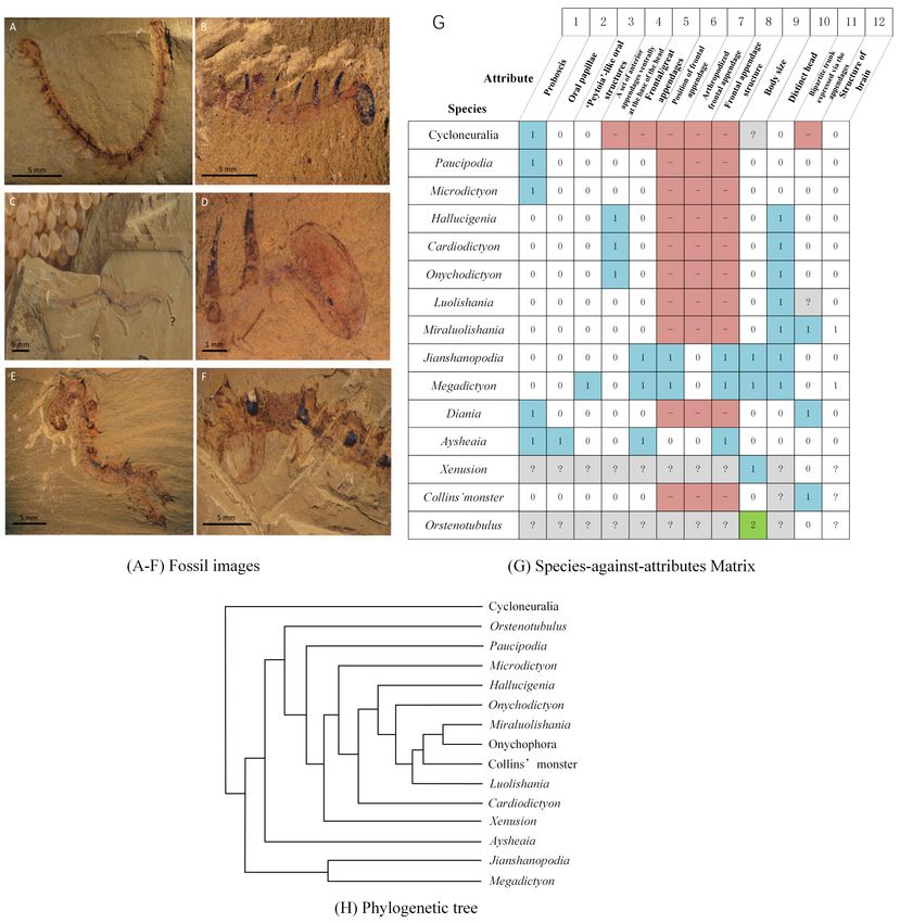
Figure 1A–H shows selected fossil images, a species-against-attributes matrix, and the results of the
phylogenetic inference analysis.
Entropy 2019, 21, 313; doi:10.3390/e21030313 www.mdpi.com/journal/entropy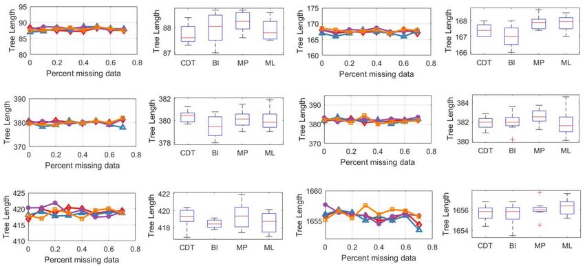
Entropy 2019, 21, 313                                                                                         2 of 17

      Figure 1. An example of phylogenetic inference. Photographs (A–F) show examples of Cambrian
      Chengjiang Lagerstätte fossils. (G) is a morphological attribute matrix, where the rows represent species
      and the columns represent attributes. In the column labels of the matrix, the first row represents the
      attribute number and the second row corresponds to the attribute name. (H) is a phylogenetic tree for
      selected lobopodians and arthropods from the early Cambrian era [1].

     Due to incomplete records, there are almost always missing values for fossils; for example, the parts
marked with “?” in image (C) in Figure 1 indicate missing data. Thus, it may be difficult to support
the results of the phylogenetic inference analysis under such circumstances. To solve this problem, four
methods have been developed to deal with missing data. First, a certain proportion of incomplete species
or attributes can be removed [2,3]. However, in many cases, the exclusion of incomplete species and
attributes is carried out in an arbitrary manner without specific explanations or reasons [3–6]. Second,
the number of attributes can be increased [7,8]. Research results showed that if the overall number of
attributes in the analysis was sufficiently large (more than 1000 attributes), a phylogenetic inference
method accurately reconstructed the position of highly incomplete taxa (e.g., 95% missing data) [2,3].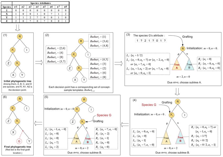
Entropy 2019, 21, 313                                                                                    3 of 17

However, due to the simple structure of early paleontology, species often have less than 200 attributes.
When the absence rate is high, a common phylogenetic inference cannot be accurately inferred. Highly
incomplete taxa may produce multiple equally parsimonious trees and poorly resolved consensus trees,
resulting in low phylogenetic accuracy [9]. Third, the missing values can be filled in. In the Hennig86 [10]
and PAUP [11] programs, for example, each unspecified attribute is randomly assigned a value that is
suitable for the attribute. Each of these three methods of dealing with missing data has its strengths and
weaknesses, but none reflect the true value of the missing data. Fourth, The species-against-feature matrix
with missing data can transform into a suitable sparse expression form by a sparse sampling algorithm,
and the reconstruction algorithm is used to reconstruct the sampling point. Sparse signal recovery theory
shows that this method can accurately reconstruct data. A common sparse representation method is
wavelet analysis [12–15]. By sparse representation of the data, wavelet analysis could potentially be
applied to the task of recovering missing phylogenetic information. It has been successfully applied to
signals, images, gene classification and so on [16,17]. However, in the study of morphological phylogenetic
analysis, it is a method that is little studied but worth trying.
      In addition, there are three main approaches based on the principle of optimality for inferring the
phylogenetic tree, namely maximum parsimony (MP) [18], maximum likelihood (ML) [19] and Bayesian
inference (BI) methods [9,20]. The ML and Bayesian methods are commonly used probabilistic approaches
based on matrices containing only gene data from living species [21]. However, since DNA is usually
not available for fossil taxa, only the fossil occurrence dates are used in time-calibrated phylogenies [22].
Moreover, researchers have found that the ML and Bayesian methods do not deal effectively with missing
morphological data [20]. MP is well known to be non-deterministic polynomial-time (NP)-hard [23]. Given
the large number of taxonomic groups, the only effective method of obtaining the optimal phylogenetic
tree is to perform a heuristic search. However, studies have shown that MP may fall into a local optimum.
Therefore, complex and flexible heuristics are needed to ensure that the tree space is fully explored.
      Our motivation is to introduce a phylogenetic inference method that reduces the impact of missing
data. In this paper, we propose an evolution analysis algorithm based on bi-directional cognitive processing;
we call this approach phylogenetic deduction based on a concept decision tree (CDT). We use a cognitive
model to reduce the search scope caused by incomplete data. In this model, a priori knowledge of
relatively complete species is used to create a highly reliable phylogenetic tree as an initial seed. Attribute
reduction [24] based on rough sets [25] is used to construct multiple concept-sample templates for each
node of the initial seed tree by removing unrelated or unimportant attributes in order to improve the
classification or decision-making [26], thereby reducing the impact of missing data. We apply a matching
algorithm to evaluate the matching degree between species’ attributes and the nodes’ concept-sample
templates; hence we determine the location of the species by a serial search in the phylogenetic tree.
Therefore, the global combinatorial explosion problem is decomposed into a classification framework that
prevents instability. Compared with the traditional parallel phylogenetic inference process applied to
all species, our method greatly reduces the computational scale and complexity of the task. Gradually,
a complete phylogenetic tree is established.
      Here we compare our method with the MP, ML, and BI methods using morphological datasets with
different amounts of missing data. We show that the proposed algorithm makes a contribution to the field
because it enables the construction of morphological data with an accuracy of 86.5% whereas the MP, ML,
and BI methods provide accuracies of 85.5%, 82.8%, and 85.1%, respectively. We also compare the stability
of the methods to establish the tree. The experimental results show that the variance of our method and
the other methods is 0.0872. Therefore, a stable phylogenetic tree can be constructed.
      The rest of the paper is organized as follows. Section 2 introduces the framework of the CDT algorithm.
The process of developing concept-sample templates based on genetic algorithms (GAs) is described in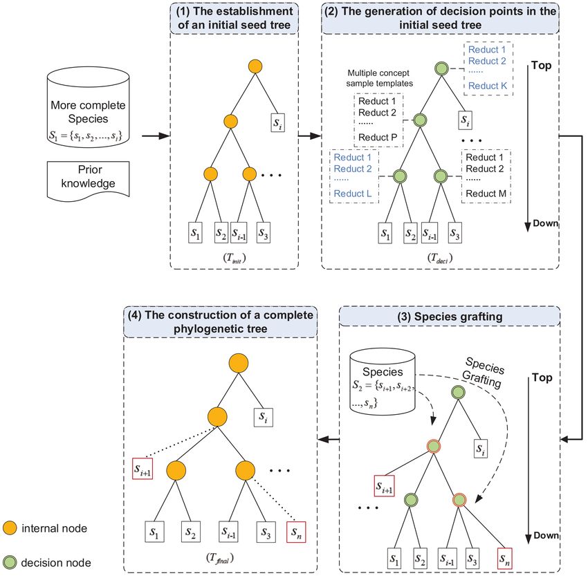
Entropy 2019, 21, 313                                                                                         4 of 17

Section 3. Section 4 presents the experimental results of the CDT and the discussion. Finally, Section 5
provides the conclusions of the study.

2. Framework of the CDT Algorithm
      The objective of the CDT algorithm is to construct a phylogenetic tree T for a set of species S,
expressed as T = (V, E) where V ← S. We input a species-against-attribute matrix SOA for a set of species
S. The species are sorted in order of completeness from high to low, which is denoted as S = {s1 , s2 , ..., sn }.
For each species s j (1 ≤ j ≤ n), there are m attributes, which are defined as A = { a1 , a2 , ..., am }. We divide
S into sub1 and sub2 , where sub1 = {s1 , s2 , ..., si } and sub2 = {si+1 , si+2 , ..., sn }. The species in sub1 are
relatively complete, whereas those in sub2 are missing many attributes.
      The framework of the phylogenetic inference based on the CDT is shown in Figure 2.

                Figure 2. The framework of phylogenetic inference based on the Concept Decision Tree.

    We divide the framework into four steps as follows:
    (1) The establishment of the initial seed tree
    Due to the ambiguity of phylogenetic tree construction, the initial concept establishment is
very important because it reduces the complexity of the subsequent steps. During the analysis of
species evolution, we first apply either biologists’ prior knowledge or common software tools (such
as MrBayes [27], PAUP* [11], or TNT [28]) to a set of relatively complete species sub1 = {s1 , s2 , ..., si } in
order to build a reliable phylogenetic tree Tinit as an initial seed, where Tinit = (V ∗ , E∗ ), V ∗ = sub1 .
    (2) The generation of decision points in the initial seed tree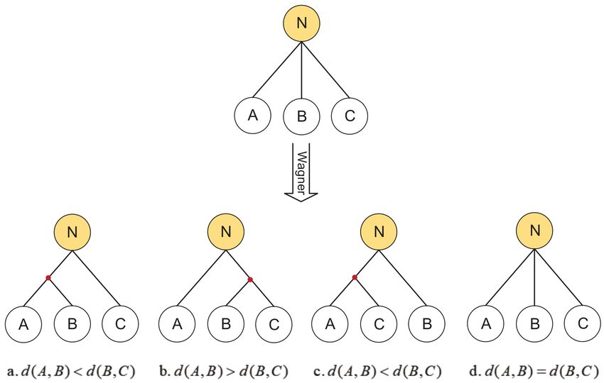
Entropy 2019, 21, 313                                                                                    5 of 17

       To take advantage of the established concepts, we perform attribute reduction on the rough set at each
branch node of the initial seed tree Tinit by analyzing the species sub1 ’ location. In this way, we obtain the
concept-sample templates for the branch nodes in Tinit . Therefore, the branch nodes have decision-making
functions that become decision points. Correspondingly, the phylogenetic seed tree becomes the decision
tree Tdeci , which provides the basis for the grafting of species with missing data.
       (3) Species grafting
       For species s j in sub2 , we can determine its location in the phylogenetic tree by matching the species’
attributes with multiple concept-sample templates of each decision point in a top-down manner.
       (4) The construction of a complete phylogenetic tree
       The evolutionary process starts with the most reliable species si+1 in sub2 , followed by grafting it
onto the tree, as described in Step 3. The next species si+2 is then added, and so on, finishing with species
sn . In this way, a complete phylogenetic tree T f inal is constructed.
       In this paper, we focus on the generation of decision points in the initial seed tree (Section 3) and
species grafting (Section 4).

3. Construction of Multiple Concept-Sample Templates
     The internal nodes in the phylogenetic tree are an important decision-making basis for phylogenetic
inference. Therefore, we transform the internal nodes into decision points. Due to a large number of
missing and inconsistent attributes, traditional pattern recognition methods are not applicable. Therefore,
a method is required to provide decision-making attribute sets for the internal nodes.
     We propose to generate multiple concept-sample templates for the internal nodes based on the species’
location. The purpose of rough set attribute reduction is to remove unrelated or unimportant attributes
in order to improve classification or decision-making [21,29]. Attribute reduction has been shown to
be an NP-hard problem for combinatorial optimization [22,23]. However, in many applications, it is
necessary to find only one minimum attribute reduction. On the other hand, because morphological data
in Paleontology are often missing many values, we need to use multiple concept-sample templates to
make full use of the data. In this study, we use entropy-based genetic algorithms (GAs) [24] to find the
optimal template sets heuristically because they can simulate the optimal solution of a natural evolutionary
process, and phylogenetic inference is essentially part of the study of evolution.

3.1. The Design of the Genetic Algorithm for Attribute Reduction
    In this section, we introduce the details of the GA to deal with attribute reduction in the
rough set theory.

3.1.1. Encoding Method
      A variable-length decimal array of one-dimensional strings represents the chromosome. The length
of the chromosome equals the number of the species’ attributes, i.e., N. Each gene bit corresponds to an
attribute in the chromosome. Each gene bit in the chromosome is numbered 1 − N, and the corresponding
code ranges from 0 to the number of the species’ attributes, where 0 denotes that the attribute is not
selected and i (0 < i < N ) denotes that the ith attribute is selected as the attribute of the concept-sample
template. The chromosomes in the initial population are generated using uniformly distributed random
numbers.
      When the length of the chromosome is N, each chromosome corresponds to a unique set of
concept-sample templates for a total of ( N + 1) N , as shown in Table 1 below: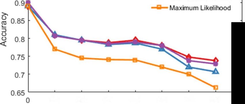
Entropy 2019, 21, 313                                                                                                                            6 of 17

                                          Table 1. The number of possible values.

          No. Attributes   No. Values                                             Possible Value
                   1             2                                                     {0} {1}
                   2            32                  {0, 0} {0, 1} {0, 2} {1, 0} {1, 1} {1, 2} {2, 0} {2, 1} {2, 2}
                   3            43           {0, 0, 0} {0, 0, 1} {0, 0, 2} {0, 0, 3} {0, 1, 0} {0, 1, 1} {0, 1, 2} {0, 1, 3}
                  ...           ...                                                         ...
                  N         ( N + 1) N        {0, 0, . . . , 0} {0, 0, . . . , 1} {0, 0, . . . , 2} . . . {0, 0, . . . , N } {0, 1, . . . , 0}

     For example, Table 2 shows the encoding method of a chromosome with N = 10. Sites 8 and 9
have the same value 9, indicating that attributes 8 and 9 belong to the same concept-sample template.
Site 10 has value 8 and the other sites have different codes; therefore, attribute 10 represents a single
concept-sample template. For example, if the template set X for a decision point is {1 3 0 4 5 7 10 9 9 8}, it
contains {1} {2} {4} {5} {6} {7} {8, 9} {10}.

                                     Table 2. Setting the chromosome bit and code.

                                    Site     1     2     3      4     5     6      7      8     9      10
                                   Code      1     3     0      4     5     7     10      9     9      8

3.1.2. Fitness Function
     The fitness of a chromosome determines the probability with which it will be inherited by the next
generation. Here, the fitness of a chromosome is calculated by reference to the concept-sample template set
generated by it. According to the principle of attribute reduction, B represents the attribute subset of the
present mapping, C = {c1 , c2 , ..., cr } represents the attribute set of the species, and D = {0, 1} represents
the class label of the species belonging to the node.

Definition 1. Let U = { x1 , x2 , ..., xn } be a non-empty finite set of objects, called the domain. X ⊆ U, X 6=                                    the
B-lower approximation set of X is defined as follows:

                                                 B (X ) = {x ∈ U | [x]R ⊆ X }                                                                       (1)

where [ x ] R denotes an equivalence class determined by object x.

Definition 2. Assuming that C, D ⊆ A, X ∈ U/D, the lower approximation set is defined as follows:

                                                 POSC ( D ) =             ∪      B (X)                                                              (2)
                                                                       x ∈U/D

That is, the lower approximation set is obtained from all of the sets contained in X.

                                                       |C |−rn
      If POSB ( D ) = POSC ( D ), we calculate           |C |
                                                                    and substitute it into the fitness function of Equation (3).
                               |C |−rn
If POSB ( D ) 6= POSC ( D ),     |C |
                                         = 0. The fitness function is defined as follows:

                                                                 L
                                                                    |C | − rn
                                                        F=      ∑      |C |
                                                                                                                                                    (3)
                                                               n =1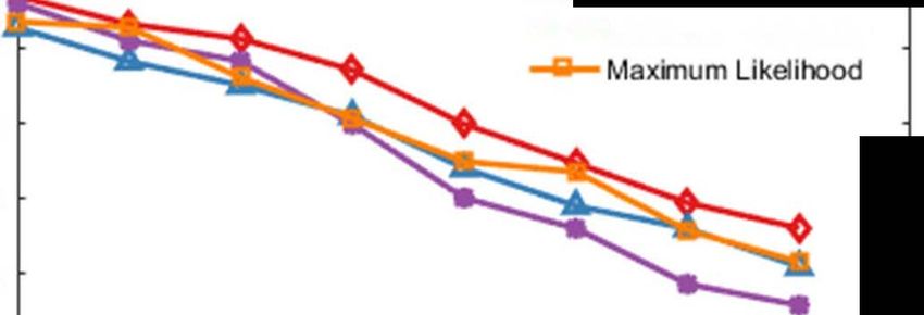
Entropy 2019, 21, 313                                                                                                    7 of 17

where L represents the number of concept template sets in the chromosome, |C | represents the number of
species attributes, n represents the nth concept-sample template, and rn represents the number of attributes
in the nth template.

3.1.3. Selection Operator
      We use the roulette wheel selection method to choose the best individual to continue to the
next generation. Individuals are selected with a probability proportional to their fitness values [30].

If a population G = X1 , X2 , ..., X pop_size (pop_size is the population size) and the fitness of the individual
Xi ∈ G is F ( Xi ), the probability of an individual Xi being selected is Pi :

                                                                           F ( Xi )
                                                               Pi =     pop_size
                                                                                                                            (4)
                                                                      ∑ j =1       F(Xj )

Pi reflects the proportion of the fitness value of the individual Xi with respect to the sum of fitness values
of all individuals.
      In order to ensure that the best individuals survive to the next generation, we use the optimal
preservation strategy [31]. If the fitness value of the worst individual in the current generation is less
than the fitness value of the best individual in the previous generation, we use the best individual in the
previous generation to replace the worst individual in the current generation. In the case of more than one
optimal individual, the optimal individual is randomly selected to replace the worst individual.

3.1.4. Crossover Operator
     The crossover operation uses a random single-point crossover strategy. An individual is chosen to
take part in the crossover at a certain probability Pc . All selected individuals are randomly paired. For each
pair of individuals, a cross-point is selected randomly. Some of the chromosomes of the paired individuals
are exchanged at the cross-point. In this way, the next generation of individuals is generated.

3.1.5. Mutation Operator
      The mutation operations use the “basic bit” variation. For each chromosome selected with probability
Pm , its mutation point is specified by a random probability and the value at the specified mutation point
becomes another state value. In this way, we can generate further members of the next generation to
improve the performance of the heuristic search.

3.1.6. Modification Operator
      Step 1: Calculate the mutual information I (C; D ) of the condition attribute set C and the decision
attribute set D. The mutual information [32] of C and D is defined as

                                                           I (C; D ) = H ( D ) − H ( D |C )                                 (5)

where H ( X )       = − ∑in=1 P( xi ) logb ( xi ) and the conditional entropy of X and Y is defined as
                                        p( xi ,y j )
H ( X |Y ) = − ∑i,j p( xi , y j ) log    p(y j )
                                                     .   When X and Y are independent, I ( X; Y ) = 0; otherwise, this index is
positive [32,33] and it increases with the degree of dependence between the components xi and yi .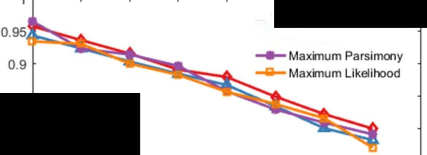
Entropy 2019, 21, 313                                                                                        8 of 17

       Step 2: Calculate I ( Reduct; D ) and I (C; D ). If I ( Reduct; D ) < I (C; D ) then repeat steps 3 and 4;
otherwise, end the modification;
       Step 3: Select attribute a in C − Reduct so that SGF(a, Reduct, D) = H(D|Reduct) − H(D|Reduct ∪ {a})
reaches the maximum value. SGF(a, Reduct, D) reflects the increment of mutual information when a is added to
Reduct. According to the definition of attribute importance of the mutual information, we select the attribute and
set it to aj;
       Step 4: Change the bit corresponding to a j from 0 to j and return to step 2;

3.2. Algorithm Description
     Input: An attribute table of Species C, the class label of the species D
     Output: Concept-sample template sets Reducti (i = 1, 2, ..., n) for each internal node
     Step 0: Set the parameters: chromosome size m, population size pop_size, crossover probability Pr ,
mutation probability Pm , and maximum generation maxgen. Let generation gen = 0.
     Step 1: Generate pop_size chromosomes randomly.
     Step 2: Calculate the fitness value of each chromosome.
     Step 3: Perform crossover on individuals selected with probability Pr .
     Step 4: Perform mutation on individuals selected with probability Pm .
     Step 5: Create the new population. Select pop_size individuals from the parents and offspring for the
next generation by the roulette wheel selection method.
     Step 6: Perform modification of the individuals.
     Step 7: Stop calculating. If gen = maxgen, then output the corresponding concept-template collection
Reducti (i = 1, 2, ..., n) and stop, else let gen = gen + 1 and return to Step 2.

4. Species Grafting Algorithm (SGA)

4.1. Description of SGA
     In the phylogenetic seed tree, the concept-sample template sets for each decision point provide
a basis for grafting the species. We calculate the matching degree of the species’ attributes and each
node’s concept-sample template sets in the phylogenetic seed tree in a top-down manner. In this way,
we can identify the location of each species in the phylogenetic seed tree and gradually complete the
grafting process.
     The process of species grafting at each decision point is shown in Figure 3. As shown in the tree
branching, the species are divided into A and B subtrees. Q represents the attribute of the grafted species.
L indicates the attribute values of the sample templates of the A subtree. R indicates the attribute values of
the sample templates of the B subtree. Let K be the number of concept-sample templates for the decision
point in the concept decision seed tree. Suppose m is the number of concept-sample templates that match
the A subtree and n is the number of concept-sample templates that match the B subtree; in this case m
and n are initialized to 0. For each of the attribute values L, R, if Li ⊆ Q (or Ri ⊆ Q), that is i.e., the species’
attribute Q contains the attribute values Li , Ri for each decision point, we can determine that Q belongs
to the A or B subtrees and let m = m + 1 (or n = n + 1). If it neither belongs to the A subtree nor the B
subtree, or it cannot be assigned because Q contains missing values, then m and n are not accumulated.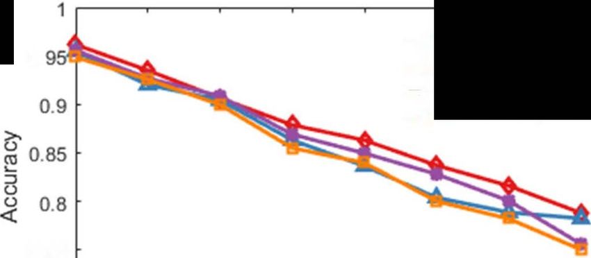
Entropy 2019, 21, 313                                                                                     9 of 17

                        Figure 3. The strategy of species grafting in a single decision node.

     When the species’ attribute Q is assigned to subtree A or subtree B of the root decision points, we
continue to perform top-down matching using the next decision point of the subtree. Using these steps,
the species’ location in the tree is determined. Finally, the species are grafted into the ultimate decision
point of the phylogenetic tree.
     In the grafted species, the proportion of missing values differs for each species. In order to obtain
a stable phylogenetic tree, the grafting is conducted one-by-one taking into account the integrity of the
species’ attributes. When all species have been grafted, a complete phylogenetic tree has been constructed.

4.2. Detailed Example of SGA
      In this section, an example is given to illustrate the specific implementation of the SGA. As shown in
Figure 4(1), an initial phylogenetic seed tree is constructed based on the species-against-attributes matrix.
Then, we use the method described in Section 3 to create multiple concept-sample templates for each
internal node in the tree, as shown in Figure 4(2). We consider the internal nodes R, N1 , N2 in order from
top to bottom. From the phylogenetic seed tree in stage (2) of the diagram, the R node divides the species
into two groups: the left subtree (species X, Y, Z) and the right subtree (species I). The concept-sample
templates of the R-node after attribute reduction are {1}, {3, 6}, {4, 8}, which means that these templates
also correctly divide the species. For example, attribute 1 divides the left subtree (X, Y, Z) and right subtree
(I); we also know from the species-against-attributes matrix that the corresponding left subtree has a value
of 1 or 2, which is recorded as the attribute value set L1 of the concept sample template. The corresponding
right subtree has a value of 0, which is recorded as the attribute value set R1 of the concept sample template
in Figure 4(3). Similarly, we can determine the attribute value set for the other sample templates.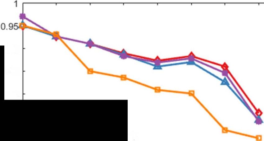
Entropy 2019, 21, 313                                                                                            10 of 17

      Figure 4. An example of the species grafting algorithm. The red dot indicates the final graft position of the
      species G.

      The grafted species G is matched with the concept-sample templates of the decision points to
determine the grafting position. The G 0 attributes are compared with the values of the node R’s left
subtree and right subtree. In (3), m and n are initialized to 0. For the first collection of attribute values
(L1 , R1 ), since a1 = 1 in species G and a1 ∈ L1 , it conforms to the left subtree Tree A; therefore, m = m + 1
provides the value 1. For the second collection of attribute values (L2 , R2 ), because a3 = 2, a6 = 0, species
G corresponds to the left subtree Tree A; therefore, m = m + 1 results in 2. For the third (L3 , R3 ), because
in the species G, a4 = 1, a8 represents missing data; therefore m and n remain unchanged. At this point,
the attribute value set traversal of node R is completed. Since m > n, the left subtree A is selected. For node
(N1 , N2 ), a similar operation is performed from the top down as shown in Figure 4(4,5). Finally, the position
of the species G grafting is determined, as shown in Figure 4(6).
      During the grafting of multiple species, it may happen that some species cannot be assigned and
grafted at the same decision point, resulting in the phenomenon of ‘species-stacking’, i.e., the creation of a
polymorphic tree. In such a case, the biologists cannot determine the interspecies relationship between the
species through the phylogenetic tree, which affects the accuracy of the evolutionary relationship. In this
study, we use the Wagner formula [34] to adjust the structure of the tree by calculating the difference
between species:
                                                        t
                                         d ( A, B) =   ∑ |X ( A, i) − X ( B, i)|                                      (6)
                                                       i =1

where d ( A, B) is the difference between species A, B; t is the number of attributes; X ( A, i ) is the state of
attribute i for species A; X ( B, i ) is the state of attribute i for species B.
Entropy 2019, 21, 313 11 of 17
As shown in Figure 5, if species A, B, and C are unions, d ( A, B) , d ( A, C ) , and d ( B, C ) are calculated.
If d ( A, B) < d ( B, C ), then A and B are closer and we merge A and B. If d ( A, B) > d ( B, C ), then B and C
are closer and we merge B and C, etc. We thereby minimize the generation of polymorphic trees.
Figure 5. An example of handling polymorphic trees.
5. Experimental Results
To assess the accuracy and reliability of the CDT, we conducted experiments on six species datasets.
The summary information for the datasets is shown in Table 3.
Table 3. Experimental data sets.
Datasets No. Species No. Attributes Reference
Pharyngodonidae 25 30 Bouamer and Morand (2003) [35]
Hibiscus 40 38 Tang et al. (2014) [36]
Meligethes 42 60 Lin et al. (2015) [37]
Nemesiid spiders 77 60 Goloboff (1995) [38]
Phrynosomatid lizards 115 59 Reeder and Wiens (1996) [39]
liebherr 160 136 Hawaiian Platynini (Carabidae), Liebherr (1998) [40]
The datasets were used to construct phylogenetic trees using our CDT algorithm as well as three other
standard methods, namely MP, ML, and BI. The specific steps are described in Section 5.1. The grafting
results of CDT were compared to the accepted tree topologies (model trees) that are part of the datasets.
The results were then compared.
5.1. CDT Accuracy Analysis
The accuracy rate of the assignment of a species, i.e., the accuracy of the species’ phylogenetic analysis,
depends on the node path of that species. The path of a species in a phylogenetic tree model accepted
by biologists is considered to be the standard path sequence Seqs . The path sequences of the grafted
species Seqc obtained from the CDT, MP, ML, and BI methods were compared with the standard path
sequences. Seqs ∩ Seqc denotes that Seqc matches the standard sequence Seqs . |Seqs ∩ Seqc | is the number
of path matching species and |Seqs | is the total number of standard sequence species. The accuracy canEntropy 2019, 21, 313 12 of 17
be expressed by Equation (7). For example, if Seqs = {1, 2, 4, 5, 8, 10} and Seqc = {1, 2, 4, 5, 8, 9}, then
acc = 56 ≈ 83.3%.
|Seqs ∩ Seqc |
acc = × 100% (7)
Seqs
To verify the performance of the CDT algorithm, the attributes of the species which are to be grafted
are randomly chosen to be incomplete. The missing proportions are 0%, 10%, 20%, 30%, 40%, 50%, 60%
and 70%. On the basis of different proportions of missing data, we apply the CDT algorithm for species
grafting and the MP, ML, and BI methods to establish phylogenetic trees. The bootstrap method [41,42] is
used to resample the data set 1000 times and the average accuracy of the four methods is calculated. For
six species datasets in Table 3, the accuracies of the four methods of phylogenetic analysis under different
proportions of missing data are shown in Figure 6.
n-
09 85 08
5e
。
5 em33V
o-
,no
85
,v
08
[
0.75
:!:�;.
氐'"
-+-Mu如mPa心吓�,
0.75 t
o,t
........,..'"
一令一CDT
-+-Mu..,mPa心而叩
--""加mLikdil"'心 .-"""'"m Likaitood
0.7 0. 65
0 01 02 0.3 0.4 0.5 06 07 0.8 0 0.1 02 03 0.4 05 06 0.7 0.8
Percent m,s�ng data Percent m;ss,ng data
(a) Pharyngodonidae (b) Hibiscus
0.95
一
一令一COT
-"-"'""''"
M"如mPa心-,
�
rn 0.85
.........,..'"
一令一COT
.,
u 08
0.75
0.7
0·55
0.1 02 0.3 0.4 0.5 0.6 0.7 0.8 O 0.1 02 0.3 0.4 0.5 0.6 0.7 0.8
Percent m;s�ng data Percent m;s�ng data
(c) Meligethes (d) Nemesiid spiders
。
-+-cor -+-cor
.........,.忒'" 0.95 ..........归'"
一.一M"m,mPa心-,
09 85 08 75 07
-+-M,.=mPa心-,
--M"如mu,.,�四
5 em33V
0 0
0.75
0.7
0·65 0. 65
o 01 02 0.3 0.4 0.5 06 07 0.8 0 0.1 02 0.3 0.4 OS 06 0.7 0.8
Percent mis�ng data Percent mis�ng data
(e) Phrynosomatid lizards (f) liebherr
Figure 6. Accuracies of phylogenetic analysis for different proportions of missing data.
We observe the following:
(1) In general, an increase in missing data results in insufficient information and a decrease in accuracy.
(2) When the proportion of missing data is less than 10%, the accuracies are similar for the different
methods, i.e., the species can be classified accurately.
(3) The proposed method significantly improves the accuracy of the results, especially for datasets
with many missing data (missing proportions > 40%). This occurs because as the species’ number of
attributes increases, the amount of data used for the concept-sample templates increases; although the
proportion of missing data increases, it is much easier to assign the species to the correct location.Entropy 2019, 21, 313 13 of 17
The average accuracies of the CDT, MP, ML and BI methods are shown in Table 4. The accuracy of
the CDT method was 86.5% whereas the accuracies of the MP, ML, and BI methods were 85.5%, 82.8%,
and 85.1%, respectively, indicating that the proposed method had the highest average accuracy.
Table 4. Average accuracies of the different methods for different data sets. The bold numbers indicate the
highest accuracy in the column.
Nemesiid Phrynosomatid
Pharyngodonidae Hibiscus Meligethes Liebherr Avg.
Spiders Lizards
BI 0.8919 0.8714 0.7828 0.8672 0.8567 0.8355 0.851
ML 0.8400 0.8250 0.7461 0.8659 0.8501 0.8428 0.828
MP 0.8990 0.8778 0.7905 0.8730 0.8618 0.8283 0.855
CDT 0.8983 0.8811 0.7930 0.8811 0.8732 0.8613 0.865
5.2. CDT Reliability Analysis
To evaluate the reliability of the CDT method, we used the tree length [43] to determine the optimality
criteria. In phylogeny, the length of the phylogenetic tree is a parameter for evaluating morphological
changes in the tree, i.e., the number of changes in the attributes. The shorter the tree length, the more
reliable the phylogenetic tree is. Therefore, a phylogenetic tree with the lowest number of changes in the
attribute state is preferred.
We used the results of the phylogenetic tree described in Section 5.1 and calculated the tree length
separately as shown in Figure 7.
Figure 7. The tree length for different proportions of missing data and for different methods.
In Figure 7, it is observed that grafted species with different proportions of missing data have little
effect on the tree length. The data in Table 5 were obtained by analyzing the results in Figure 7.
Table 5 shows that the tree length of the phylogenetic tree is similar for all four methods and the
average variance of the tree length is 0.0872. Therefore, our method is as reliable as the other methods.Entropy 2019, 21, 313 14 of 17
Table 5. The variance of tree length between the CDT algorithm and that calculated by the other
three methods.
Nemesiid Phrynosomatid
Pharyngodonidae Hibiscus Meligethes Liebherr Avg.
Spiders Lizards
CDT vs. BI 0.0282 0.0800 0.4278 0.0282 0.0800 0.0500 0.1157
CDT vs. ML 0.0153 0.0957 0.0488 0.0153 0.0957 0.0180 0.0481
CDT vs. MP 0.1250 0.1128 0.0282 0.1250 0.1128 0.0821 0.0977
5.3. Phylogenetic Inference on Cambrian Lobopodians
In this study, we apply the CDT to the phylogenetic analysis of the Cambrian lobopodians.
The Cambrian lobopodians paleontological morphological dataset [1] contains large amounts of missing
data; for example, the species Opabinia has 32% missing data, while Hadranaxa and Orstenotubulus have
48% missing data. The species Opabinia, Hadranaxa, and Orstenotubulus were sequentially used for grafting
to construct phylogenetic trees, as shown in Figure 8. The results show that our method provides a
phylogenetic tree that is consistent with the assessment of paleontologists.
Figure 8. A paleontological phylogenetic tree. The red solid dot is the node position and the position of the
red square is the grafting position of the species.Entropy 2019, 21, 313 15 of 17
6. Conclusions
In this paper, we used bi-directional cognitive and concept-driven processing for the process of
phylogenetic inference. Using prior knowledge of phylogenetic analysis, we generated a phylogenetic
seed tree and used genetic attribute reduction to construct concept-sample template sets for each decision
point using a top-down algorithm. Subsequently, top-down template matching was used to determine the
grafting position of the species containing missing values in the phylogenetic seed tree. The experimental
results show that the CDT method had high accuracy and stability and resulted in a phylogenetic tree that
was familiar to biologists. The proposed method solves the problem of creating a stable phylogenetic tree
when much of the data are missing.
Author Contributions: Conceptualization, J.F.; methodology, J.F. and Z.L.; formal Analysis, Z.L.; writing—original
draft, J.F. and Z.L.; writing—review and editing, Z.L. and R.F.E.S; funding acquisition, J.L. and J.H.
Funding: This research was funded by the 973 Project of the Ministry of Science and Technology of China
Grant number 2013837100 and the National Natural Science Foundation of China Grant number 41621003.
Acknowledgments: The authors would like to thank the editor and the reviewers for their insightful suggestions.
Conflicts of Interest: The authors declare no conflict of interest.
References
1. Liu, Y.Y.; Jeanjacques, S.; Albertlászló, B. Liu et al. reply. Nature 2011, 478, E4–E5. [CrossRef]
2. Wiens, J.J. Does adding characters with missing data increase or decrease phylogenetic accuracy? Syst. Biol.
1998, 47, 625–640. [CrossRef] [PubMed]
3. Wiens, J.J. Incomplete taxa, incomplete characters, and phylogenetic accuracy: Is there a missing data problem?
J. Vertebr. Paleontol. 2003, 23, 297–310. [CrossRef]
4. Livezey, B.C. Phylogenetic relationships and incipient flightlessness of the extinct Auckland Islands Merganser.
Wilson Bull. 1989, 101, 410–435.
5. Hufford, L.; Dickison, W.C. A phylogenetic analysis of Cunoniaceae. Syst. Bot. 1992, 17, 181–200. [CrossRef]
6. Smith, A.B.; Paterson, G.L.; Lafay, B. Ophiuroid phylogeny and higher taxonomy: Morphological, molecular and
palaeontological perspectives. Zool. J. Linn. Soc. 1995, 114, 213–243. [CrossRef]
7. Hillis, D.M.; Huelsenbeck, J.P.; Cunningham, C.W. Application and accuracy of molecular phylogenies. Science
1994, 264, 671–677. [CrossRef] [PubMed]
8. Kearney, M.; Clark, J.M. Problems due to missing data in phylogenetic analyses including fossils: A critical
review. J. Vertebr. Paleontol. 2003, 23, 263–274. [CrossRef]
9. Wiens, J.J. Missing data, incomplete taxa, and phylogenetic accuracy. Syst. Biol. 2003, 52, 528–538. [CrossRef]
[PubMed]
10. Farris, J. Hennig86, Version 1.5.; Distributed by the author; Port Jefferson Station: New York, NY, USA, 1988.
11. Swofford, D. PAUP*: Phylogenetic Analysis Using Parsimony and Other Methods (Software); Sinauer Associates:
Sunderland, MA, USA, 2000.
12. Mallat, S.G. A theory for multiresolution signal decomposition: The wavelet representation. IEEE Trans. Pattern
Anal. Mach. Intell. 1989, 7, 674–693. [CrossRef]
13. Guido, R.C.; Addison, P.S.; Walker, J. Introducing wavelets and time-frequency analysis. IEEE Eng. Med.
Biol. Mag. 2009, 28, 13. [CrossRef] [PubMed]
14. Daubechies, I. Ten Lectures on Wavelets; Society for Industrial and Applied Mathematics: Philadelphia, PA, USA, 1992.
15. Newland, D.E. Harmonic wavelet analysis. Proc. R. Soc. Lond. Ser. A Math. Phys. Sci. 1993, 443, 203–225.
[CrossRef]
16. Guariglia, E.; Silvestrov, S. Fractional-Wavelet Analysis of Positive definite Distributions and Wavelets on D 0 (C );
Springer: Berlin, Germany, 2016.Entropy 2019, 21, 313 16 of 17
17. Guariglia, E. Spectral analysis of the Weierstrass-Mandelbrot function. In Proceedings of the 2nd International
Multidisciplinary Conference on Computer and Energy Science (SpliTech), Split, Croatia, 12–14 July 2017.
18. Fitch, W.M. Toward defining the course of evolution: Minimum change for a specific tree topology. Syst. Biol.
1971, 20, 406–416. [CrossRef]
19. Felsenstein, J. Evolutionary trees from DNA sequences: A maximum likelihood approach. J. Mol. Evol. 1981,
17, 368–376. [CrossRef] [PubMed]
20. Wiens, J.J. Missing data and the design of phylogenetic analyses. J. Biomed. Inf. 2006, 39, 34–42. [CrossRef]
[PubMed]
21. Guillerme, T.; Cooper, N. Effects of missing data on topological inference using a total evidence approach.
Mol. Phylogenet. Evol. 2016, 94, 146–158. [CrossRef] [PubMed]
22. Zuckerkandl, E.; Pauling, L. Molecules as documents of evolutionary history. J. Theor. Biol. 1965, 8, 357–366.
[CrossRef]
23. Foulds, L.R.; Graham, R.L. The Steiner problem in phylogeny is NP-complete. Adv. Appl. Math. 1982, 3, 43–49.
[CrossRef]
24. Blum, A.L.; Langley, P. Selection of relevant features and examples in machine learning. Artif. Intell. 1997,
97, 245–271. [CrossRef]
25. Pawlak, Z. Rough sets. Int. J. Comput. Inf. Sci. 1982, 11, 341–356. [CrossRef]
26. Ma, X.; Wang, G.; Yu, H. Heuristic method to attribute reduction for decision region distribution preservation.
J. Softw. 2014, 8, 1761–1780.
27. Huelsenbeck, J.P.; Ronquist, F. MRBAYES: Bayesian inference of phylogenetic trees. Bioinformatics 2001,
17, 754–755. [CrossRef] [PubMed]
28. Goloboff, P.A.; Farris, J.S.; Nixon, K.C. TNT, a free program for phylogenetic analysis. Cladistics 2008, 24, 774–786.
[CrossRef]
29. Yang, Z.; Rannala, B. Bayesian phylogenetic inference using DNA sequences: A Markov Chain Monte Carlo
method. Mol. Biol. Evol. 1997, 14, 717–724. [CrossRef] [PubMed]
30. Tsujimura, Y.; Gen, M. Entropy-based genetic algorithm for solving TSP. In Proceedings of the
Second International Conference. Knowledge-Based Intelligent Electronic Systems, Adelaide, SA, Australia,
21–23 April 1998; Volume 2, pp. 285–290.
31. Zhengjiang, W.; Jingmin, Z.; Yan, G. An attribute reduction algorithm based on genetic algorithm and
discernibility matrix. J. Softw. 2012, 7, 2640–2648.
32. Arellano-Valle, R.B.; Contreras-Reyes, J.E.; Genton, M.G. Shannon entropy and mutual information for
multivariate skew-elliptical distributions. Scand. J. Stat. 2013, 40, 42–62. [CrossRef]
33. Cover, T.M.; Thomas, J.A. Elements of Information Theory; John Wiley and Sons: Hoboken, NJ, USA, 2012.
34. Lipscomb, D. Basics of Cladistic Analysis; George Washington University: Washington, DC, USA, 1998.
35. Bouamer, S.; Morand, S. Phylogeny of palaearctic pharyngodonidae parasite species of testudinidae:
A morphological approach. Can. J. Zool. 2003, 81, 1885–1893. [CrossRef]
36. Tang, L.D.; Yuan, M.M.; Yan, L.I.; Wang, X. Phylogenetic analysis of hibiscus based on morphological characters.
J. Henan Agric. Sci. 2014, 43, 105–111.
37. Lin, X.L.; Chen, Y.; Huang, M.; Yang, X.K. A new species of the genus Meligethes Stephens (Coleoptera:
Nitidulidae: Meligethinae) from China. Zool. Syst. 2015, 40, 268–289.
38. Goloboff, P.A. A Revision of the South American Spiders of the Family Nemesiidae (Araneae, Mygalomorphae). Part 1,
Species from Peru, Chile, Argentina, and Uruguay. Bulletin of the AMNH; no. 224; American Museum of Natural
History: New York, NY, USA, 1995.
39. Reeder, T.W.; Wiens, J.J. Evolution of the lizard family Phrynosomatidae as inferred from diverse types of data.
Herpetol. Monogr. 1996, 10, 43–84. [CrossRef]
40. Liebherr, J.K.; Zimmerman, E.C. Cladistic analysis, phylogeny and biogeography of the Hawaiian Platynini
(Coleoptera: Carabidae). Syst. Entomol. 1998, 23, 137–172. [CrossRef]
41. Efron, B.; Tibshirani, R.J. An Introduction to the Bootstrap; CRC Press: Boca Raton, FL, USA, 1994.Entropy 2019, 21, 313 17 of 17
42. Davison, A.C.; Hinkley, D.V. Bootstrap Methods and Their Application; Cambridge University Press: Cambridge, UK,
1997; Volume 1.
43. Huang, D.W. An Introduction to Cladistics; China Agriculture Press: Beijing, China, 1996.
c 2019 by the authors. Licensee MDPI, Basel, Switzerland. This article is an open access
article distributed under the terms and conditions of the Creative Commons Attribution (CC
BY) license (http://creativecommons.org/licenses/by/4.0/).You can also read