Tutorial - Petrophysics Module - Cyclolog
←
→
Page content transcription
If your browser does not render page correctly, please read the page content below
Tutorial – Petrophysics Module

        PanTerra – ENRES Technical Alliance ● CycloLog Version 2021 ● Petrophysics Module ● Page 1
Contents

Part 1 – Log analysis and processing functions ............................................................................... 4
          1.1       Log analysis and processing in Cyclolog ............................................................................................ 4
          1.2 Using CycloLog’s analysis functions ........................................................................................................... 4
          1.2       Log calculations ................................................................................................................................. 6
          1.4 Log filters ................................................................................................................................................... 9
          1.5 Using the Erode and Deposit functions ................................................................................................... 11

Part 2 - Log spectral analysis functions .......................................................................................... 14
          2.1 Log spectral analysis in CycloLog ............................................................................................................. 14
          2.2 Introduction to CycloLog’s spectral analysis functions ........................................................................... 14
          2.3 Using spectral analysis in CycloLog.......................................................................................................... 15
          2.4 Interpretation of Milankovitch cycles ..................................................................................................... 19
          2.5 Using the MESA menu ............................................................................................................................. 21

Part 3 - Advanced log processing functions ................................................................................... 23
          3.1 Advanced processing functions in CycloLog ............................................................................................ 23
          3.2 Generating synthetic seismograms ......................................................................................................... 23
          3.3 Using Math Studio ................................................................................................................................... 24
          3.4 Markov Chain Analysis in CycloLog ......................................................................................................... 29

Part 4 - Basic petrophysical functions ............................................................................................ 33
          4.1 Petrophysical functions in CycloLog ........................................................................................................ 33
          4.2 Porosity calculation ................................................................................................................................. 33
          4.3 Porosity calculation from a density log ................................................................................................... 33
          4.4 Porosity calculation from density and neutron logs................................................................................ 35
          4.5 Porosity calculation from a sonic log ....................................................................................................... 37
          4.6 Porosity calibration ................................................................................................................................. 39
          4.7 Permeability calculation .......................................................................................................................... 41
          4.8 Water saturation calculation ................................................................................................................... 42
          4.9 Water resistivity calculation .................................................................................................................... 43
          4.10 Generate petrophysical report .............................................................................................................. 43

Part 5 - Total Organic Carbon (TOC) .............................................................................................. 46
          5.1 TOC calculation method in CycloLog ....................................................................................................... 46
          5.2 TOC workflow in CycloLog ....................................................................................................................... 46
          References ..................................................................................................................................................... 50

                                                          PanTerra – ENRES Technical Alliance ● CycloLog Version 2021 ● Petrophysics Module ● Page 2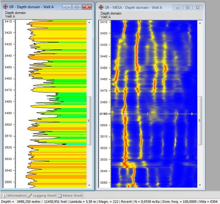
Copyright © 2021 PanTerra Geoconsultants B.V. All rights reserved
No part of this document may be reproduced or transmitted in any form or by any means, electronic or
mechanical, for any purpose, without written consent of PanTerra Geoconsultants. Under the law,
reproducing includes translating into another language or format. As between the Parties, PanTerra
Geoconsultants retains title to, and ownership of, all proprietary rights with respect to the software
contained within its products. The software is protected by copyright laws. Therefore, you must treat the
software like any other copyrighted material (e.g., a book or sound recording). Every effort has been made
to ensure that the information in this user guide is accurate. PanTerra Geoconsultants is not responsible
for printing or clerical errors. Information in this document is subject to change without notice.

CycloLog and INPEFA are registered trademarks of ENRES Energy Resources International BV and PanTerra
Geoconsultants BV.

                                    PanTerra – ENRES Technical Alliance ● CycloLog Version 2021 ● Petrophysics Module ● Page 3
Part 1 – Log analysis and processing functions
1.1 Log analysis and processing in Cyclolog
CycloLog contains a wide range of functions for analysing and processing log data. Here we describe how
to use the more basic functions; the use of some of the more advanced functions is described in the parts
that follow.
1.2 Using CycloLog’s analysis functions
Under the right-click menu of the log data pane, the following three functions in the Analysis menu are
found:
Accumulated thickness
Log statistics
Histogram
The Histogram function is not discussed here. Refer to the Tutorial – Clustering and Lithology, part 2.
The Accumulated thickness function is used to calculate the total thickness of a section where the log
value lies in a user-specified range. This function can be used for calculations of, for example, net-to-gross.
In the example on the next pages, the user is interested in the cumulative thickness of sand in the interval
between the two markers 4000-4100 and 5000-5100. The user has decided to take a cut-off value of 60
API. The task, then, is to calculate the depth interval for which the value of the GR log is less than 60. To
do this:
Open the log to be analysed (in this case, the GR log).
Place the cursor on the log, open the right-click menu and select Analysis → Accumulated thickness.
The following dialog box opens:
PanTerra – ENRES Technical Alliance ● CycloLog Version 2021 ● Petrophysics Module ● Page 4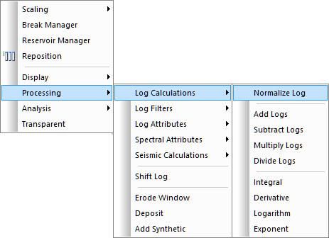
The default depth interval is the entire log: to change this, enter the Top and Bottom depths of the
interval to be analysed.
Enter the Cut-off log value (60 in this example).
The Minimum and Maximum log values (here set to 0 and 150) allow the user to exclude any
unwanted outlying values.
Click Recalculate. The Analysis results box gives the cumulative thickness of the intervals for which
the log value is below (interval 1) and above (interval 2) the cut-off value. The results are given both
in depth units, and as percentages.
If one or more sets of breaks (see Tutorial – Base Module, part 5) have been defined, it may be easier to
specify the interval to be analysed in terms of defined breaks, as follows:
Open the log to be analysed (in this case, the GR log).
Place the cursor on the log, open the right-click menu and select Analysis → Accumulated thickness.
At the top of the Accumulated Thickness dialog box, click the Break button.
For the breaks that define the Top and Bottom depths of the interval to be analysed, select the break
set and break, as in the example below:
PanTerra – ENRES Technical Alliance ● CycloLog Version 2021 ● Petrophysics Module ● Page 5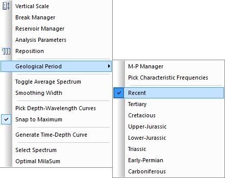
Click Recalculate, and read the results as described above.
The Log statistics function calculates from the minimum and maximum log data values the average, root
mean square (RMS), and standard deviation in a user-defined depth interval.
Open the log to be analysed (in this case, the GR log).
Place the cursor on the log, open the right-click menu and select Analysis → Log Statistics.
Enter the Top and Bottom Depth intervals (default = whole log).
Click Recalculate. The statistic results will be
Note that the calculated values cannot be saved.
1.2 Log calculations
A number of basic mathematical functions are available in Log Calculations. Mathematical operations can
be performed for each log Data Pane. The basic mathematical operations available appear in the log data
pane right-click menu; select Processing → Log Calculations:
PanTerra – ENRES Technical Alliance ● CycloLog Version 2021 ● Petrophysics Module ● Page 6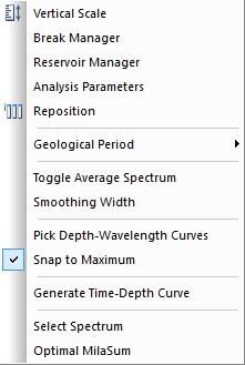
All Log Calculation operations can be undone (and redone) using any of the following actions:
Edit → Undo (Redo); the menu shows the name of the last action
Undo (Redo) icon on the Standard toolbar
ALT + backspace
Several successive actions can be undone/redone (the number is more or less unlimited), and CycloLog
maintains a separate record of actions for each log data pane. This information is retained, both when you
save the project, and also if you close and then re-open the data pane without saving the project.
Normalize Log - Using this option, logs can be normalized as a preparation for e.g., Clustering.
PanTerra – ENRES Technical Alliance ● CycloLog Version 2021 ● Petrophysics Module ● Page 7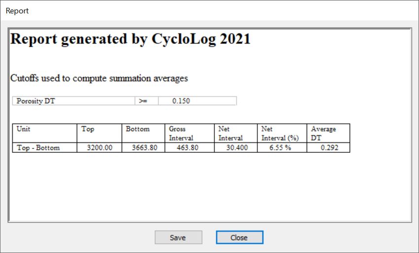
In the Normalize GR menu above, Minimum and Maximum log values are shown. These are the minimum
and maximum measured values of a certain property (e.g., GR) that were measured within the depth
interval specified further down the menu. Even though different values for the Minimum and Maximum
can be entered, these manual entries are not applied in any calculations.
The depth interval that you want to use for normalisation can be specified by:
Providing depth values for the top and bottom of the interval, or
Specifying a complete interval (Reservoir) at once.
To provide depth values, check the button Depth Values. To specify the top of the interval you want to
use for normalisation, either select Use depth or Use break from the drop-down menu. When Use break
is selected, an interval can be selected that is added above the break. To specify the bottom of the interval,
follow the same workflow as for specifying its top.
When you click OK, the normalised log will be saved to the workspace as norm – .
To use a reservoir interval for normalisation, select the button Interval and specify a reservoir you defined
earlier (see Tutorial – Base Module, part 6). It is optional to add an interval above and below the specified
reservoir.
PanTerra – ENRES Technical Alliance ● CycloLog Version 2021 ● Petrophysics Module ● Page 8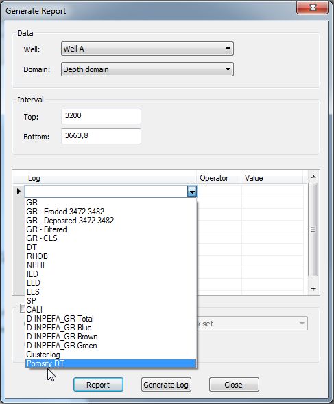
The log value at the Top depth will be used as the minimum for normalisation, the log value at the Bottom
will be used as the maximum for normalisation.
Next to normalisation, CycloLog can perform some basic binary mathematical operations on log data.
These are launched from the Processing dialog, which is accessed from the log display.
Add Logs (add one log to another).
Subtract Logs (subtract one log from another).
Multiply Logs (multiply one log by another).
Divide Logs (divide one log by another).
Integral (calculate the integral of a log curve).
Derivative (calculate the derivative of a log curve).
Logarithm (calculate the logarithm of all data values in a log).
Exponent (calculate the inverse logarithm of all data values).
These functions are straightforward in their use in CycloLog analysis and will not be further discussed here.
They are all launched from the Processing menu, which is accessed from the log display right-click menu.
In the CycloLog Help manual you can find more details of these functions.
1.4 Log filters
Filtering of log data has a variety of applications, such as smoothing the logs, and enhancing certain
wavelengths in the data. Filtering may also be useful in conjunction with frequency analysis (see part 2).
To use log filters, you should first make a duplicate of the log to be processed, in order to keep a copy of
the original data.
Right-click over the name of the log in the workspace.
PanTerra – ENRES Technical Alliance ● CycloLog Version 2021 ● Petrophysics Module ● Page 9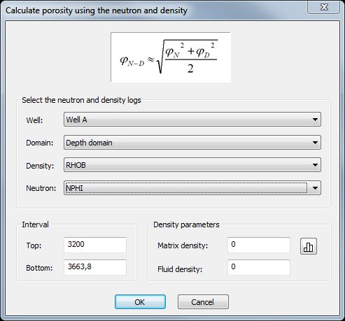
Click Duplicate.
(To move the new log up the list, drag it to the required place in the list.)
A copy of the log is added to the list in the workspace; double-click on the log to open it.
Right-click over the log data pane, and select Processing → Log Filters.
Select the type of filter to be used: in the illustrated example, the Median Filter was used.
In the dialog box, enter the length of the window of analysis to be used (5 was used in the example;
the default is 3), and click OK.
In the processed log, each log value is now replaced with (in this case) the median of the 5 values in
a window centred at that depth.
All log processing operations, including filtering, can be undone: click the Undo button on the
Standard toolbar. The Undo operation will apply to the currently active log display pane.
If you plan to keep the result, rename the processed log: right-click over its name in the workspace,
select Rename, type the new name, and press the Enter key.
PanTerra – ENRES Technical Alliance ● CycloLog Version 2021 ● Petrophysics Module ● Page 101.5 Using the Erode and Deposit functions
The Erode and Deposit functions respectively remove section from a log, and add synthetic section to a
log. They can be useful for comparing logs from wells in which the succession is similar, but part of the
section in one of the wells is missing (because of faulting, say, or non-deposition).
To ‘erode’ section from a log:
In case you want to keep both a copy of the original and the newly created log, make a duplicate of
the original log.
Open the duplicate log.
Right-click over the log data pane, and select Processing → Erode Window.
In the dialog box, enter the Top and Bottom depths of the interval to be removed.
Click OK.
To undo the ‘erode’ operations, click the Undo button on the Standard toolbar. The Undo operation
will apply to the currently active log display pane.
The result is shown below: the shaley interval between 3472m and 3482m has been removed, and the
lower part of the log has been moved up to close the gap.
PanTerra – ENRES Technical Alliance ● CycloLog Version 2021 ● Petrophysics Module ● Page 11To ‘deposit’ a section within a log:
In case you want to keep both a copy of the original and the newly created log, make a duplicate of
the original log.
Open the duplicate log.
Right-click over the log data pane, and select Processing → Deposit.
In the dialog box, enter the depth at which section is to be added, and the thickness of the section to
be added.
Click OK.
To undo the ‘erode’ operations, click the Undo button on the Standard toolbar. The Undo operation
will apply to the currently active log display pane.
In the example below, 10m of section has been interpolated into the log at a depth of 3472m. Note that
this adds 10m to the depths of all data-points below this point.
PanTerra – ENRES Technical Alliance ● CycloLog Version 2021 ● Petrophysics Module ● Page 12PanTerra – ENRES Technical Alliance ● CycloLog Version 2021 ● Petrophysics Module ● Page 13
Part 2 - Log spectral analysis functions
2.1 Log spectral analysis in CycloLog
CycloLog’s unique contributions to well log analysis lie in its spectral functions. Spectral analysis exploits
methods that are commonly referred to as time-series analysis. Time-series (waveform) data have
properties of wavelength (or frequency), amplitude and phase. (Frequency is the inverse of wavelength.)
A well log, treated as a composite waveform, has properties of wavelength, amplitude and phase that can
be analysed through the methods of spectral analysis.
This approach also underlies the calculation of the PEFA and INPEFA curves, as described in the Tutorial –
Base Module, part 3. Indeed, the Prediction Error Filter exploited by PEFA and INPEFA is directly related
to the power spectrum calculated using the Maximum Entropy method, as outlined below.
The main purpose of spectral analysis of well log data is the search for stratigraphic cyclicity. In favourable
circumstances, stratigraphy may respond to climatic change. An important driver of climate change is the
periodic changes in insolation caused by predictable changes in Earth’s orbit – the so-called Milankovitch
cyclicity. CycloLog has special tools to assist the detection of such cyclicity in log data.
2.2 Introduction to CycloLog’s spectral analysis functions
Spectral analysis decomposes a composite waveform into a set of simple sine and cosine waves.
Because the spectral properties of geological data are not constant throughout a well, it is appropriate to
use a sliding-window approach. This means that the analysis is performed repeatedly for successive, and
usually overlapping, ‘windows’ of the data. The length of the window is typically a few tens of meters (the
default value in CycloLog is 40m, though this can be changed by the user). Starting from the bottom, the
analysis is performed on the lowest (say) 40m of the data, then the window is moved up (by, say, 1m) and
the analysis is repeated, all the way up to the top of the data.
The oldest and most familiar spectral analysis method is Fourier Analysis. The methods available are in
CycloLog are:
Fourier Transform
Maximum Entropy
Wavelet (Gabor)
Wavelet (Modified)
Walsh Transform
The Fourier Transform of a waveform is its exact equivalent in the frequency domain. Fourier analysis is
appropriate for data – such as radio waves – that can be expected to conform to continuous sine and
cosine waves.
The Maximum Entropy approach is different and is often referred to as spectral estimation. (The entropy
of a dataset is related to its information content.) However, the results can be expressed in the form of a
power spectrum, in exactly the same way as the results of a Fourier analysis. Thus, the difference of
approach need not concern the average user of CycloLog.
PanTerra – ENRES Technical Alliance ● CycloLog Version 2021 ● Petrophysics Module ● Page 14 The Maximum Entropy approach is more appropriate to stratigraphic data, (which is much less likely
to conform to regular sines and cosines) and we recommend its use in most cases.
The method is also called MESA (for Maximum Entropy Spectral Analysis).
Wavelet approaches to spectral analysis attempt to model the power spectrum at a single point. In
practice this is not possible, but the concept is obviously relevant to stratigraphic data, in which the
properties can be expected to change abruptly, at hiatuses and boundaries for example. CycloLog includes
two different wavelet methods, the details of which (and the differences between them) are not likely to
be important to the average user.
The Walsh Transform treats the data-series as the composite of a number of square waves, which is a
rather different approach to the other methods, and its use is too specialized to be described in detail
here. However, the resulting Walsh power spectra are similar to the power spectra from the other
methods, and there is no reason why the interested user should not experiment with the method.
2.3 Using spectral analysis in CycloLog
The use of spectral methods in CycloLog is illustrated here with the Maximum Entropy method, which is
the one recommended for general use. While some of the details are different for the other methods,
most of the following applies equally to all methods.
To launch any of the spectral methods, go to the main menu bar and select Analysis → Frequency Analysis.
This opens the Frequency Analysis dialog box:
In the Method tab, check that the correct well and log are selected from the drop-down lists, and
select Maximum Entropy from the list of Methods.
In the Parameters tab, you have to set some important parameters for the analysis:
PanTerra – ENRES Technical Alliance ● CycloLog Version 2021 ● Petrophysics Module ● Page 15It will be necessary to experiment with the parameters; the following guidelines may help:
Window is the length of the analysis window in depth units: start by using the default value (40m).
(Note: when your data is in feet, use 120ft).
The default Start and End depths include the entire log: change the depths if you wish to analyse only
a part of the data.
The Step size is the amount (in depth units) by which the window is moved at each step in the
calculation. Start with the default value (1m). (Note: when your data is in feet, use 3ft).
The Autocorrelation length should be set to approximately a quarter of the window length. (The
default value for window length 40m is 9m.) (Note: when your data is in feet, use 27ft).
The values of Minimum and Maximum Wavelength define the range of values shown on the
horizontal scale of the finished power spectrum. Start with the defaults and adjust to different values
if the results are not satisfactory.
Vertical scaling is best kept to the default value of 1.
In many cases, the power of the smaller wavelengths will be swamped by the large ones: in such cases
check the Enhance small wavelengths box to correct for this effect.
When all parameters are set, click OK in the Frequency Analysis dialog box.
CycloLog runs the spectral analysis, and adds the result to the list of logs in the workspace. The name of
the new “log” will be, for example, GR – MESA. If you run a second analysis, its name will be GR – MESA
(2).
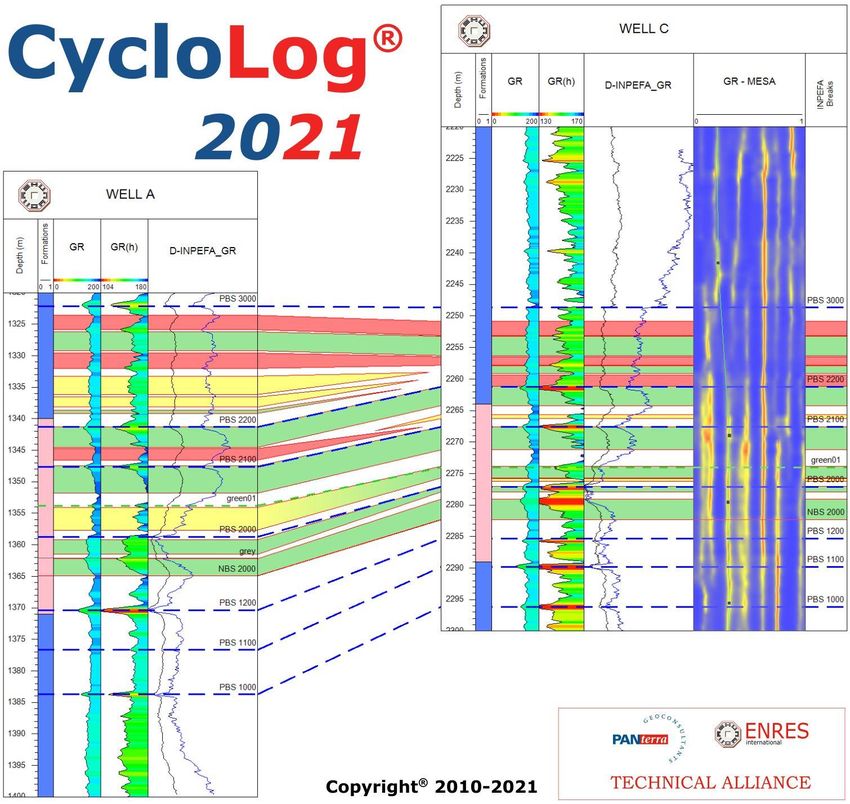
PanTerra – ENRES Technical Alliance ● CycloLog Version 2021 ● Petrophysics Module ● Page 16To open the MESA results, double-click on its name in the workspace. The example below shows the result
of a MESA analysis (Right pane) on the GR log displayed in the left pane. The vertical axis of the MESA
display is depth, and the display scrolls with other logs from the same well.
To interpret the results, remember that the method uses a moving window of analysis. The power spectra
resulting from analysis of each window are stacked up, such that the peaks in successive spectra line up
to form ridges in the stack. The peaks are coloured to represent their relative height (i.e. amplitude), so
that higher spectral ridges appear as brightly coloured streaks on the display.
The horizontal scale of the display represents wavelength, decreasing logarithmically from left to right.
(Longer wavelengths on the left; shorter wavelengths towards the right.) A vertical streak of bright colour
indicates a wavelength that is persistently present through that interval of the log data.
Although no horizontal scale is shown on the display, the wavelength of any peak at any depth can be
found by using the cursor, as follows:
To view the power spectrum at a single depth, move the cursor over the MESA log pane. The cursor
changes into a horizontal line with five tick marks:
PanTerra – ENRES Technical Alliance ● CycloLog Version 2021 ● Petrophysics Module ● Page 17From this menu, select Toggle Average Spectrum.
PanTerra – ENRES Technical Alliance ● CycloLog Version 2021 ● Petrophysics Module ● Page 18The Average Spectrum window opens. This window shows the Average Amplitude Spectrum, or power
spectrum, at a single depth point (in the image above, at depth 5352.179m); the spectrum changes as the
cursor is moved up and down the GR - MESA data pane.
The Amplitude is scaled vertically; the Wavelength (m) is shown on the horizontal axis, where it is plotted
logarithmically, from higher values on the left, to lower values at the right.
2.4 Interpretation of Milankovitch cycles
The result of a spectral analysis is a breakdown of the data into a set of simple (sine/cosine) waves.
Deciding whether or not these have any geological and/or climatic significance is a matter of
interpretation.
PanTerra – ENRES Technical Alliance ● CycloLog Version 2021 ● Petrophysics Module ● Page 19E1 E2 O P1 P2
When the cursor is over the MESA display, it takes the form of a horizontal line with five tick marks, as in
the above figure. The relative positions of the ticks represent (in terms of wavelength) the ratios among
the principal predicted Milankovitch frequencies. For different Periods, the obliquity and precession cycles
vary. For recent times these are:
E1, long orbital eccentricity cycle: 413ka
E2, short eccentricity cycle: 100ka
O, axial obliquity cycle: 41ka
P1, precession cycle: 23ka
P2, precession cycle: 19ka
Note that the logarithmic scale makes the 413ka and 100ka tick marks appear closer together than the
23ka and 19ka ticks!
Note also that the relative positions of the predicted Milankovitch periods are also shown on the Average
Amplitude Spectrum display: see the figure above in part 3.2.
By default, the 100ka tick is selected as the “dominant” frequency: it is distinguished from the others, by
having a cross line through it. To change the dominant frequency, see further below.
The Status Bar displays the frequency (Dom. freq.) and amplitude (Magn.) of the power spectrum at the
point under the “dominant” tick mark.
PanTerra – ENRES Technical Alliance ● CycloLog Version 2021 ● Petrophysics Module ● Page 20The Status Bar also provides two statistics designed to help in the identification of Milankovitch periods:
Sedimentation rate: this is the net accumulation rate implied by the wavelength position
corresponding to the position of the “dominant frequency” tick mark on the Milankovitch cursor (N
= 0.0551 m/ka on the figure above). This assumes, of course, that deposition was continuous and at
an unchanging rate, so must be used with care.
MilaSum (“Mila” on the Status Bar) is an arbitrary measure of the quality of the match between the
predicted Milankovitch period ratios, and the ratios between the observed peaks, for the current
position of the Milankovitch cursor. This statistic should also be used with care, but it may help with
choosing between different interpretations.
If a full suite of Milankovitch periods is perfectly represented in the stratigraphy, then the corresponding
peaks in the MESA spectrum should all lie under one of the ticks on the Milankovitch cursor. Moving the
cursor ticks with the mouse should indicate whether or not this is likely. Bear in mind that any
interpretation in terms of Milankovitch cycle periods must be consistent with available evidence for the
total duration of the succession.
It is very rarely the case that all Milankovitch periods are represented. The user will therefore have to
decide, (a) whether any of the spectral wavelengths are likely to represent Milankovitch periods, and, if
so, (b) which wavelengths correspond to which of the predicted cycle periods.
2.5 Using the MESA menu
Place the cursor over the GR - MESA data pane and right-click with the mouse to open a menu that contains
a number of special functions.
Analysis parameters shows a record of the parameters used to generate the MESA display.
Toggle Average Spectrum was explained above; it can be toggled on/off.
Geological Period (illustrated below). The ratios between the Milankovitch periodicities change
through geological time; select the period most appropriate to the data being analysed. (See CycloLog
Help for further information.)
M-P Manager (on the Geological Period menu). Use this dialog box to change the periodicity selected
as “dominant” (default – 100ka).
PanTerra – ENRES Technical Alliance ● CycloLog Version 2021 ● Petrophysics Module ● Page 21PanTerra – ENRES Technical Alliance ● CycloLog Version 2021 ● Petrophysics Module ● Page 22
Part 3 - Advanced log processing functions
3.1 Advanced processing functions in CycloLog
CycloLog has a number of additional/advanced calculation and analysis functions. Introductory
instructions for some of these functions are given in this section of the tutorial; others are explained in
CycloLog Help. The functions covered here are:
Synthetic seismogram – generating simple seismic traces from logs
Math Studio – defining arithmetical combinations of logs
Markov Chain Analysis – analysing patterns of upward change
3.2 Generating synthetic seismograms
Synthetic seismic traces can be generated in CycloLog, either automatically or manually. The automatic
method is described here; the manual method is described in CycloLog Help.
Go to the main menu bar and select Calculations → Synthetic Seismogram. The following dialog
window opens:
Select the Well you wish to calculate a synthetic seismogram. Check the Domain.
From the Sonic and Density drop-down lists, select the sonic and density logs that you wish to use in
the calculation.
Select a Wavelet – see below for information.
Define the Wavelength (default = 10m). Click OK.
PanTerra – ENRES Technical Alliance ● CycloLog Version 2021 ● Petrophysics Module ● Page 23 The Synthetic Seismogram is generated, and added to the workspace.
The above figure shows the synthetic seismogram displayed alongside the sonic and density curves from
which it was generated. The display initially shows only a single trace, without toning. This is converted to
a multiple trace display (as shown above) as follows:
Make sure the synthetic seismogram pane is open and the active pane.
Open the properties pane.
Under Log appearance, set the Display mode to Pseudo section.
Under Toning, set Use toning to True and set the Toning side, Tone color and Cutoff value.
Note: Wavelet types available in the Synthetics Seismogram dialog are:
Minimum Phase Wavelet
Ricker Wavelet Type 1 (the standard Ricker wavelet)
Ricker Wavelet types 2, 3 and 4 (Ricker wavelets with a more “ringing” character)
3.3 Using Math Studio
The Math Studio consists of a range of calculations that can be performed on logs.
Several basic calculations can be performed without using the Math Studio. Their use was described in
part 1.3 of this tutorial, and they are:
PanTerra – ENRES Technical Alliance ● CycloLog Version 2021 ● Petrophysics Module ● Page 24 Add Logs (add one log to another)
Subtract Logs (subtract one log from another)
Multiply Logs (multiply one log by another)
Divide Logs (divide one log by another)
Integral (calculate the integral of a log curve)
Derivative (calculate the derivative of a log curve)
Logarithm (calculate the logarithm of all data values in a log)
Exponent (calculate the inverse logarithm of all data values)
For the above calculations, open the log that is to be the subject of the calculation (suggestion: use a copy
of the log), right-click over the opened log pane and select Processing → Log Calculations and then select
the required operation.
For more advanced calculations, use the Math Studio, as follows:
From the main menu bar select Tools → Math Studio.
The Math Studio dialog box opens. It a number of tabs and other features, briefly explained in the
following figure below.
The Math Studio is used to set up formulas that will be applied to every depth point in a specified
interval.
The formulas can be set up by selecting the logs, the arithmetical operators, various available functions,
and a selection of constants, from standard lists.
PanTerra – ENRES Technical Alliance ● CycloLog Version 2021 ● Petrophysics Module ● Page 25 The Equations tab is where you will set up a formula, as in the example described below.
The Logs tab has a list of all the logs of the selected well in the workspace, including logs that you
have created such as cluster logs or synthetic seismograms.
The Constants tab lists four basic constants (DZ, PI, ZMAX, and ZMIN).
The Operators tab lists ten basic arithmetical operators (add, subtract etc.).
The Functions tab lists twenty-six more advanced functions, including trigonometrical functions (sine,
cosine, etc.), logarithms (natural and base 10), and exponentiation.
To demonstrate how to set up an equation, the following example calculates shale separation from the
neutron and density curves, using the formula: 100*NPHI/0.6 + RHOB - 2.7. (This formula assumes that
NPHI is expressed as a ratio; where NPHI is a percentage, the formula is NPHI/0.6 + RHOB - 2.7).
Go to the Equations tab.
Click in the Equation field, at the bottom of the dialog box.
The following sequence of operations will construct the equation:
Type 100.
Go to the Operators tab and double-click on the multiply operator (*). Note that this operator is
added to the Equation field.
PanTerra – ENRES Technical Alliance ● CycloLog Version 2021 ● Petrophysics Module ● Page 26 Go to the Logs tab and double-click on the NPHI log.
Go to the Operators tab and double-click on the add operator (/).
Type 0.6.
Go to the Operators tab and double-click on the add operator (+).
Go to the Logs tab and double-click on the RHOB log.
Go to the Operators tab and double-click on the subtract operator (-).
Type 2.7.
The full formula now appears in the Equation field, as:
To save this formula:
Click the Add button to open the Save Equation Dialog box.
Type a name for the formula, and click OK.
The formula has been saved for future use; it will now appear on the Equations tab every time you open
the Math Studio.
PanTerra – ENRES Technical Alliance ● CycloLog Version 2021 ● Petrophysics Module ● Page 27To apply the formula:
Check that the correct Well is selected at the top of the dialog box.
Check that the equation is listed in Equation field (if not double-click on “Shale separation” in the
equation list.
Change the depth Interval if you do not want the formula applied to the entire data set.
Click Calculate.
CycloLog runs the calculation, and adds the results to the workspace as a new log with the name of
the formula (in this case, the new log is called “Shale Separation”).
To save the formula for importing to another CycloLog project:
Select the formula in the list on the Equations tab.
Click Export and give the file a name (e.g., ShaleSeparation).
The file will be saved as (for example) ShaleSeparation.equ.
PanTerra – ENRES Technical Alliance ● CycloLog Version 2021 ● Petrophysics Module ● Page 283.4 Markov Chain Analysis in CycloLog
Markov Chain Analysis in general looks for relationships between the current state of a process and its
previous state. In stratigraphy, it is used for testing the relationships between adjacent lithologies in a
stratigraphic succession: is the succession of lithologies purely random, or is there some order to the way
in which lithologies succeed each other?
No single log has a direct relationship with lithology; it is therefore necessary to start by defining the
‘lithologies’ that the Markov Chain Analysis will work with. There are several ways to do this, but a good
starting point is a Cluster Analysis, as described in Tutorial – Clustering and Lithology, part 1.
The following description of a Markov Chain Analysis in CycloLog is based on the result of the cluster
analysis that was used as an example in the Tutorial – Clustering and Lithology, part 1.
The native clustering was based on the combination of the GR, sonic, neutron and density logs; it defined
seven clusters.
From the main menu bar select Analysis → Markov Chain Analysis.
On the General tab of the dialog box, select the Well and the Log on which the analysis will be based;
in the example, this is the Cluster Log.
Define the Top and Bottom depth interval for the analysis.
Define the Step size; this is the size of the intervals into which the data will be divided into ‘lithologies’
(1 meter in the example).
Now open the Lithology tab.
PanTerra – ENRES Technical Alliance ● CycloLog Version 2021 ● Petrophysics Module ● Page 29 Accept the default method: Automatic. See below concerning the other methods (Predefined model,
and Manual).
For the log on which the analysis is to be based, identify the Minimum and Maximum values of the
log in the interval to be analysed. (In the example, the clusters are numbered from 0 to 7, so the
minimum is 0 and the maximum is 7.)
Define the Number of Intervals (i.e. ‘lithologies’) into which the data are to be divided (7 in the
example). Click OK.
The analysis runs, and a Markov Chain Log is added to the list in the workspace. (This depicts the
‘lithologies’ into which the chosen log has been subdivided for the analysis.)
The figure above shows the Cluster log (middle pane) which was used as the basis for subdivision into
lithologies. In the Markov Chain Log (right hand pane), 7 ‘lithologies’ (based on the clusters) are defined
in 1m steps. The Markov Chain Analysis categorizes every upward transition, at every 1m step, and counts
the resulting transitions.
To view the results of the analysis:
Open the new Markov Chain Log.
Right-click over the opened Markov Chain Log pane and select Analysis Results.
The following Markov Chain Analysis Results dialog box opens:
PanTerra – ENRES Technical Alliance ● CycloLog Version 2021 ● Petrophysics Module ● Page 30The analysis categorises and counts every upward transition from one lithology to the next. Note that,
because all steps are the same size (1m in the example), many of the upward transitions will be “self-
transitions”, at which the lithology stays the same. Based on these counts, the probability of every possible
upward transition is calculated; if the data are not random, then some upward transitions will be more
likely than others.
The results box presents this information in three parts, two on the Matrix tab and one on the Significance
tab.
On the Matrix tab, the table of Observed transition probabilities shows the relative probabilities of every
possible upward transition. (See the data on the Significance tab for the details of these results.) The table
should be read from row to column. A few of these results are now discussed, to suggest how the results
might be interpreted.
In the example, lithology 1 is succeeded by itself with a high probability of 0.980. Lithology 1 has the
characteristics of e.g. a fine-grained sandstone; the high probability of an upward “self-transition”
means that such sandstones are likely to occur in units greater than 1m in thickness.
Lithologies 3 and 4 have lower probabilities of self-transition, so are more likely to occur in thinner
beds.
PanTerra – ENRES Technical Alliance ● CycloLog Version 2021 ● Petrophysics Module ● Page 31 Lithology 5 has a high probability (0. 382) of upward transition to lithology 3, but zero probability of
upward transition to lithology 1.
Lithology 4 is quite likely (0.350) to be succeeded by lithology 2, but lithology 2 is much less likely
(0.085) to be followed by lithology 4.
Based on these transition probabilities, the Markov chains box on the Matrix tab shows the possible
upward chains of lithological states, in decreasing order of their probability. Each such chain is a “cycle”
in that it starts and finishes with the same lithology. In the example, there is a large number of possible
chains, indicating that there is no one dominant cyclic or repetitive pattern. Looking at the first few in the
example, and taking the Cluster Matrix of the Cluster Log analysis results into account (see below):
The chain 3 > 1 > 3 occurs with the highest probability. Lithologies 1 and 3 both have low GR values,
so this chain expresses the moderate probability of switching between sandstones with slightly higher
and slightly lower GR values.
The next three chains are 3 > 2 > 3 with probability 0.171; and 5 > 3 > 2 > 5 (0.146). They represent
variations on transitions among lithologies with mid- to high-range GR values.
The following two chains contain rather more abrupt transitions: 5 > 2 > 5 (0.146); and 5 > 4 > 2 > 5
(0.146). Lithologies 2 and 5 are considerably more different in their GR values.
PanTerra – ENRES Technical Alliance ● CycloLog Version 2021 ● Petrophysics Module ● Page 32Part 4 - Basic petrophysical functions
4.1 Petrophysical functions in CycloLog
CycloLog includes a number of basic petrophysical functions. Introductory instructions for these are given
in this section of the tutorial. Functions covered here are:
Porosity calculation
Porosity calibration using core measurements
Permeability calculation
Water saturation calculation
Water resistivity calculation
Creating a petrophysical summary report
4.2 Porosity calculation
In CycloLog, there are three different ways for calculating porosity estimations, starting from the following
logs:
Density log
Sonic log
Density and neutron logs
You may wish to use more than one of these methods, depending on which logs are available, and to
compare the results.
All three options are selected from the Porosity menu:
Go to the main menu bar and select: Petrophysics → Porosity.
Move the cursor to the Porosity item you wish to use.
Select the required method.
4.3 Porosity calculation from a density log
Calculation of porosity (φdensity) from a density log uses the following formula:
φdensity = (ρmatrix – ρbulk) / (ρmatrix – ρfluid)
PanTerra – ENRES Technical Alliance ● CycloLog Version 2021 ● Petrophysics Module ● Page 33where,
ρmatrix = matrix (or grain) density
ρbulk = bulk density as measured by the logging tool
ρfluid = density of fluid
As long as we can provide numbers for the matrix density (ρmatrix) and the fluid density (ρfluid), this formula
will give the porosity (in fraction between 0.0 and 1.0) from the density log (ρbulk).
If the lithology of the matrix is known, use the following standard density values (in g/cm3):
Sandstone (quartz) 2.648
Limestone (calcite) 2.710
Dolomite 2.850
Gypsum 2.351
Anhydrite 2.977
Halite 2.032
For the fluid density, use 1.0 g/cm3 for freshwater, and 1.1 g/cm3 for brine.
Alternatively, the matrix density can be obtained directly from the log data, as explained below.
To start the calculation:
From the main menu bar, select: Petrophysics → Porosity;
Then select Use Density Log.
The following dialog box opens:
PanTerra – ENRES Technical Alliance ● CycloLog Version 2021 ● Petrophysics Module ● Page 34 Check that the correct Well is selected.
Select the required density log from the drop-down list.
Specify the Top and Bottom depth interval over which the porosity is to be calculated.
Enter the Fluid density (in g/cm3). See above.
EITHER enter the Matrix density (if known).
OR average the Matrix density from the data as follows:
Click on the Histogram icon next to the Matrix density box.
Hold the cursor over the value regarded as representing the appropriate density value, and click
once with the left mouse button
A vertical red line marks the currently selected value.
Click OK to enter this value into the Matrix density box in the Calculate porosity dialog box.
Click OK to run the porosity calculation.
CycloLog runs the calculation and creates a new log called Porosity (here: RHOB) that is saved
to the workspace.
4.4 Porosity calculation from density and neutron logs
The second method available in CycloLog calculates porosity (in %) from a combination of a density and a
neutron log. The combined porosity (φN - D) is calculated as the root-mean-square of the porosities from
the density and neutron logs separately:
φN - D = ((φN2 + φD2) / 2)1/2
If the lithology of the matrix is known, use the following standard density values (in g/cm3):
PanTerra – ENRES Technical Alliance ● CycloLog Version 2021 ● Petrophysics Module ● Page 35Sandstone (quartz) 2.648
Limestone (calcite) 2.710
Dolomite 2.850
Gypsum 2.351
Anhydrite 2.977
Halite 2.032
For the fluid density, use 1.0 g/cm3 for freshwater, and 1.1 g/cm3 for brine.
Alternatively, the matrix density can be obtained directly from the log data, as explained below.
To start the calculation:
From the main menu bar, select: Petrophysics →Porosity.
Then select Use Density and Neutron Log.
The following dialog box opens:
Check that the correct Well is selected.
Select the required Density log from the drop-down list.
Select the required Neutron log from the drop-down list.
Specify the Top and Bottom depth interval over which the porosity is to be calculated.
Enter the Fluid density (in g/cm3).
EITHER enter the Matrix density (if known).
OR average the Matrix density from the data as follows:
Click on the Histogram icon next to the Matrix density box.
PanTerra – ENRES Technical Alliance ● CycloLog Version 2021 ● Petrophysics Module ● Page 36 Hold the cursor over the value regarded as representing the appropriate density value, and click
once with the left mouse button.
A vertical red line marks the currently selected value.
Click OK to enter this value into the Matrix density box in the Calculate porosity dialogue box.
Click OK to run the porosity calculation.
CycloLog runs the calculation and creates a new log called Porosity (here: RHOB-NPHI). This
log is added to the workspace tree.
4.5 Porosity calculation from a sonic log
Porosity (φsonic) may also be calculated from a sonic log if no density log is available, although the results
may be less reliable. The calculation is based on the following formula:
φsonic = (Δtlog – Δtmatrix) / (Δtfluid – Δtmatrix)
where,
Δtlog = sonic log value (interval transit time)
Δtmatrix = interval transit time for the matrix
Δtfluid = interval transit time for the fluid
Given values for the interval transit time in the matrix and the pore fluid, this formula allows us to calculate
sonic porosity from the values of the sonic log.
If the lithology of the matrix is known, you may be able to use one of the following standard values (in
μs/ft) for Δtmatrix:
Sandstones (quartz) 55.5 – 51.0
Limestone (calcite) 53 – 47.6
Dolomite 43.5
Gypsum 52 – 53
Anhydrite 50
Halite 67.0
For the fluid interval transit time, use 189 μs/ft for freshwater-based mud, or 185 μs/ft for saltwater-based
mud.
Alternatively, the matrix interval transit time can be obtained directly from the log data, as explained
below.
To start the calculation:
From the main menu bar, select: Petrophysics → Porosity.
Then select Use Sonic Log.
The following dialog box opens:
PanTerra – ENRES Technical Alliance ● CycloLog Version 2021 ● Petrophysics Module ● Page 37 Check that the correct Well is selected.
Select the required Sonic log from the drop-down list.
Specify the Top and Bottom depth interval over which the porosity is to be calculated.
Enter the Fluid interval transit time (in μs/ft);
EITHER enter the Matrix interval transit time (if known).
OR average the Matrix interval transit time from the data as follows:
Click on the Histogram icon next to the Matrix interval transit time box.
Hold the cursor over the peak regarded as representing the appropriate sonic value, and click once
with the left mouse button.
A vertical red line marks the currently selected value.
Click OK to enter this value into the Matrix interval transit time box in the Calculate porosity dialog
box;
Click OK to run the porosity calculation.
PanTerra – ENRES Technical Alliance ● CycloLog Version 2021 ● Petrophysics Module ● Page 38CycloLog runs the calculation and creates a new log called Porosity (here: DT). This log is shown
in the following illustration beside the original sonic (DT) log:
4.6 Porosity calibration
If direct porosity measurements are available (from core samples, for example), these can be used to
calibrate a log-derived porosity curve.
Suppose that the following porosities have been measured on a core of the selected well, at the given
depths:
PanTerra – ENRES Technical Alliance ● CycloLog Version 2021 ● Petrophysics Module ● Page 39Depth Porosity
3220m 0.25
3225m 0.04
3331m 0.02
3365m 0.18
From the main menu bar, select Petrophysics → Calibrate Porosity.
In the dialog box that opens, select Well and Porosity log to be calibrated. Click Next.
The Calibration with Core Plug Porosities dialog box opens:
Enter the Depths and core porosity measurements (Por. Core) in the first and second columns.
(Alternatively, if you have the values in a table like the one above, copy it to the clipboard, and click
the Import button to paste the values into the dialog box).
Click Calculate, and CycloLog enters the porosity values from the selected log.
(You can choose either to Interpolate between the values at the nearest depths, or Shift to nearest,
to use the log value at the nearest available depth).
Click Next.
A graph of Core Porosity against Log Porosity opens, in which the black line represents a reference
line when no calibration is needed, and the red line shows the relationship as calibrated with the core
porosity measurements.
The regression equation for the calibrated relationship is shown.
Use the Print and Export buttons to print the graph, or to export it as an image file.
PanTerra – ENRES Technical Alliance ● CycloLog Version 2021 ● Petrophysics Module ● Page 40 If the graph is acceptable, click Finish to apply the calibration to all the points in the porosity log.
The calibrated log is saved in the workspace as (for example) Porosity RHOB-calibrated.
4.7 Permeability calculation
Calculation of permeability in CycloLog requires (1) a porosity log, and (2) some core permeability
measurements.
The steps are the same as for Calibrate Porosity, above. That is:
From the main menu bar, select Petrophysics → Permeability.
In the Calculate Permeability dialog, select the porosity log to be used (and the Top and Bottom
depth interval, if relevant).
Click Next.
In the Permeability dialog box, enter the Depth and Permeability values for each available core
permeability measurement.
Click Calculate to find the corresponding log porosity values.
Click Next.
The graph and regression equation show the resulting relationship between core permeability and
log porosity: if this is acceptable, click Finish.
CycloLog applies the equation to all log values (in the specified depth interval) and creates a new log
called, for example, Permeability from Porosity RHOB-NPHI.
PanTerra – ENRES Technical Alliance ● CycloLog Version 2021 ● Petrophysics Module ● Page 414.8 Water saturation calculation
Calculation of water saturation in CycloLog requires (1) a porosity log, and (2) the formation resistivity
curve (or a deep resistivity log).
To run a water saturation calculation:
From the main menu bar, select Petrophysics → Water Saturation → Water Saturation.
The Calculate Water Saturation dialog box opens:
The box shows the formula used to calculate water saturation.
Under Input logs, select the Well, its Domain, the Formation resistivity log and the Porosity log to
be used.
Under Interval, enter the Top and Bottom depths of the interval of calculation.
Add a non-zero value for the Water resistivity.
Either accept the default values for the Tortuosity factor, Cementation exponent, and Saturation
exponent, or enter your preferred values.
Click OK.
CycloLog calculates the new log, and saves it in the workspace as Water Saturation Curve.
PanTerra – ENRES Technical Alliance ● CycloLog Version 2021 ● Petrophysics Module ● Page 424.9 Water resistivity calculation
Calculation of water resistivity in CycloLog requires (1) a porosity log, and (2) the formation resistivity
curve (or a deep resistivity log).
To run a water saturation calculation:
From the main menu bar, select Petrophysics → Water Saturation → Water Resistivity Curve.
The Water Resistivity Curve dialog box opens:
Under Input logs, select the Well, its Domain, the Formation resistivity log and the Porosity log to
be used.
Under Interval, enter the Top and Bottom depths of the interval of calculation.
Either accept the default values for the Tortuosity factor, and Cementation exponent, or enter your
preferred values.
Click OK;
CycloLog calculates the new log and saves it in the workspace as Water Resistivity Curve.
4.10 Generate petrophysical report
The Petrophysical Report function in CycloLog can be used to generate a simple N/G report, or other
similar types of report.
The report can be generated for a total interval, or the total interval can be subdivided, the subdivisions
being based on a pre-defined set of either Breaks (see Tutorial – Base Module, part 5), or Reservoirs (see
Tutorial – Base Module, part 6).
To generate a Petrophysical Report:
Go to the main menu bar and select: Analysis → Report.
PanTerra – ENRES Technical Alliance ● CycloLog Version 2021 ● Petrophysics Module ● Page 43 The Generate Report dialog box opens:
In the example above, the analysis will look for all depths in the Porosity DT log for which the value is
greater than or equal to 15.
Specify the Top and Bottom depth interval for the analysis.
Click a row under the column Log, to reveal a drop-down list.
Select the log you wish to analyse.
Click under Operator and select the operator to be used (>=, meaning greater-than-or-equal-to, in
the example illustrated).
Under Value, enter the target value (0,15 in the example).
Click Report.
The following window opens:
PanTerra – ENRES Technical Alliance ● CycloLog Version 2021 ● Petrophysics Module ● Page 44This shows the results of the analysis: for the specified depth interval, the criterion Porosity ≥ 15% is
satisfied in 30.4m out of the total of 463.8m, with an average N/G of 0.0655 in the net interval.
Click Save to save these results to a file, then
Click Close to close the report window.
The Generate Report dialog also offers a Generate Log button. This generates a simple log in which the
value 1 indicates that the condition (e.g., Porosity ≥ 15%) is satisfied at that depth, and 0 indicates that it
is not satisfied. The log is added to the workspace, and is called Report Log.
This log can be used, for example, to colour a GR log to show the intervals in which the porosity is
greater than 15%. (Open the GR log, open the properties pane, under Log Fill select Fill with. Select Log
and then select the Report Log in the dropdown menu).
PanTerra – ENRES Technical Alliance ● CycloLog Version 2021 ● Petrophysics Module ● Page 45Part 5 - Total Organic Carbon (TOC)
5.1 TOC calculation method in CycloLog
The Total Organic Carbon (TOC) curve is calculated in CycloLog based on the method as described in Passey
et al. (2009). This method, the Δ log R technique, applies the overlaying of a porosity log on a resistivity
curve. In their paper, a combination of the transit-time curve (sonic, in µsec/ft) and resistivity curve (in
ohm) is used.
The following log combinations can be used in CycloLog:
resistivity – sonic
resistivity – neutron
resistivity – density
Note that each log must be specified in the following units:
Resistivity : ohm
Sonic : µsec/ft
Neutron : V/V (0-100)
Density : g/cm3
5.2 TOC workflow in CycloLog
In this workflow, the resistivity and the sonic curves are used to calculate the TOC content in a well. The
curves will be overlain and baselined in a fine-grained, ‘non-source’, rock interval. With the baseline
established, organic-rich intervals can be recognised by separation of the two curves, which is the Δ log R.
The Δ log R is linearly related to TOC and is a function of maturity. Therefore, the maturity (in level of
organic metamorphism units, LOM) is needed. If the LOM value is not known, it can be derived from
measured vitrinite reflectance values (Hood et al., 1975). The well should be subdivided into several
intervals, if multiple (and different) levels of maturity are present.
To determine TOC, start with displaying the resistivity and the sonic curve in an overlay pane:
In the main menu bar, select View → Log Overlay.
Select from the Log Overlay View dialogue box the logs to be displayed: the resistivity and sonic logs.
PanTerra – ENRES Technical Alliance ● CycloLog Version 2021 ● Petrophysics Module ● Page 46You can also read