Light up your data using PI DataLink 2019 with Excel's advanced features - PI World 2020 Lab

PI World 2020 Lab

Light up your data using PI DataLink 2019 with
 Excel’s advanced features

Operational IntelligenceCopyright
Copyright & Trademark
© Copyright 1995-2020
OSIsoft, LLC
1600 Alvarado Street
San Leandro, CA 94577

© 2020 by OSIsoft, LLC. All rights reserved.

All rights reserved. No part of this publication may be reproduced, stored in a retrieval system, or transmitted, in any form or by any means,
mechanical, photocopying, recording, or otherwise, without the prior written permission of OSIsoft, LLC.
OSIsoft, the OSIsoft logo and logotype, Managed PI, OSIsoft Advanced Services, OSIsoft Cloud Services, OSIsoft Connected Services, PI ACE, PI
Advanced Computing Engine, PI AF SDK, PI API, PI Asset Framework, PI Audit Viewer, PI Builder, PI Cloud Connect, PI Connectors, PI Data
Archive, PI DataLink, PI DataLink Server, PI Developers Club, PI Integrator for Business Analytics, PI Interfaces, PI JDBC Driver, PI Manual
Logger, PI Notifications, PI ODBC Driver, PI OLEDB Enterprise, PI OLEDB Provider, PI OPC DA Server, PI OPC HDA Server, PI ProcessBook, PI
SDK, PI Server, PI Square, PI System, PI System Access, PI Vision, PI Visualization Suite, PI Web API, PI WebParts, PI Web Services, RLINK and
RtReports are all trademarks of OSIsoft, LLC.

All other trademarks or trade names used herein are the property of their respective owners.

U.S. GOVERNMENT RIGHTS
Use, duplication or disclosure by the US Government is subject to restrictions set forth in the OSIsoft, LLC license agreement and/or as
provided in DFARS 227.7202, DFARS 252.227-7013, FAR 12-212, FAR 52.227-19, or their successors, as applicable.

Published: March 18, 2020

2|Page

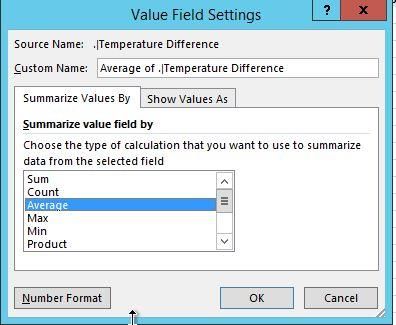
Table of Contents

Contents
Table of Contents .................................................................................................................................................................... 3
1. INTRODUCTION ............................................................................................................................................................... 6
 Workspace & File Locations .................................................................................................................................... 6
 The Fictitious Plant Used in This Lab ....................................................................................................................... 6
 How to use this Workbook...................................................................................................................................... 9
 Useful Resources ..................................................................................................................................................... 9
2. EXERCISE: Create a Report using PI DataLink................................................................................................................ 10
 Objectives.............................................................................................................................................................. 10
 Background ........................................................................................................................................................... 10
 Calculation Functions in PI DataLink ..................................................................................................................... 11
 Solutions................................................................................................................................................................ 13
3. EXERCISE: Analyze Downtime Events using PivotCharts and PivotTables .................................................................... 15
 Objectives.............................................................................................................................................................. 15
 Background ........................................................................................................................................................... 15
 Directed Activity: Retrieve Event Frames in Excel using PI DataLink .................................................................... 15
 Directed Activity: Create PivotTables and PivotCharts ......................................................................................... 17
 3.4.1 Comparing Downtime Events Based on Reason Code .................................................................................. 17
 3.4.2 Comparing Downtime Events Based on Tank ............................................................................................... 21
 Analyze Downtime Events Using PivotTables and PivotCharts............................................................................. 23
 Bonus: Making Reports More User-Friendly......................................................................................................... 24
 Solutions................................................................................................................................................................ 25
4. EXERCISE: Improve Performance of Large Workbooks ................................................................................................. 26
 Objectives.............................................................................................................................................................. 26
 Background ........................................................................................................................................................... 26
 Directed Activity: Measure AF SDK calls made in the background ....................................................................... 27
 Directed Activity: Gather information about the workbook ................................................................................ 31
 Improve performance by reducing the number of background calls ................................................................... 33
 Solutions................................................................................................................................................................ 35
5. EXERCISE: Excel’s New Dynamic Array Functions ......................................................................................................... 36
 Objectives.............................................................................................................................................................. 36

Background ........................................................................................................................................................... 36
 Learn about Excel’s new dynamic array functions................................................................................................ 37
 Use dynamic array functions to complement PI DataLink functions .................................................................... 38
 Solutions................................................................................................................................................................ 39
6. EXERCISE: Introduction to PI DataLink Documentation ................................................................................................ 41
 Objective ............................................................................................................................................................... 41
 Background ........................................................................................................................................................... 41
 Access PI DataLink’s user guide in context ........................................................................................................... 42
 Directed Activity: Access the Customer Portal ..................................................................................................... 43
 Save the Date! ................................................................................................................... Error! Bookmark not defined.

4|Page

5|Page

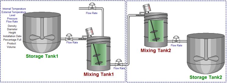
1. INTRODUCTION

This lab is designed for users who are familiar with Microsoft Excel and have already
used PI DataLink.
Learn how to combine the power of PI Datalink with Excel's advanced features such
as sparklines, Pivot Tables, Pivot Charts, and dynamic arrays. Using these tools, we
will show you best practices for creating reports and examples to prepare PI System
data and event frames for root cause analysis.

 Workspace & File Locations
Each lab attendee has their own client machine but will be using the same PI Data
Archive and AF Server, PISRV1. All machines are VMs hosted in an Azure Virtual
Learning Environment (VLE).
A soft copy of this workbook is available on the desktop of your client machine. As it
contains several hyperlinks, you are encouraged to copy the workbook from your lab
client machine to your laptop. (The clipboard is enabled through Remote Desktop
connections)
When you first log in to your lab VM, open Excel. You will be prompted to log in; use
the O365 test account credentials provided on your Connection Sheet. After
successfully logging in, go to File > Account > Update Options > Update Now to
ensure you are running the latest version. In the About Excel info, you should see the
Monthly Channel and at least Version 2001, which corresponds to the January 30th
release that rolled out new functions we will use in Exercise 5.

 The Fictitious Plant Used in This Lab
In this lab, we will have a fictitious plant named OSIsoft Plant. This simple plant has
two production lines, where each has a combination of one mixing tank and one
storage tank. This plant could be schematically shown as:

6|Page

Introduction

 OSIsoft Plant

 Production Area
 Production Line 1 Production Line 2

As shown here, each tank has different process variables such as Internal and
External Temperatures, Flow Rate, Pressure and Level whose values are
continuously collected from devices on the Plant. In the early days of PI System,
these process variables were the only data items whose historical data could be
stored in Data Archive.
There are some other data associated with each of these tanks such as the
manufacturer, model and the installation date which are stored in the maintenance
sheets available on tables in SQL Server. Moreover, all the information related to the
material flowing in these tanks is kept in tables on the Plant’s SQL Servers.
Even though these tables are available on the SQL server, their information could
not easily be integrated with the historical data stored in Data Archive. Hence, using
AF and hierarchy becomes critical in bringing all the important data and information
in one place: the PI System.
At the OSIsoft Plant, predictions on the level of each mixing tank is critical in running
a smooth production. This data, Level_Forecast, is stored in a “Future” point on the
Data Archive and could be viewed on PI System displays or be compared to the
actual value of level in any PI Application.

 7|Page

A collection of PI Points are built on Data Archive for storing the values of process
variables. There is also a hierarchy built in AF for this Plant, bringing all the important
information and data, including the process variable time series data, to one place.

8|Page

Introduction

 How to use this Workbook
This workbook is structured around exercises. Each exercise will begin with
objectives and background sections, then proceed through a variety of individual
exercises, directed activities, and questions. Solutions for exercises and questions
are available at the end of the overall exercise; directed activities guide you through
the solution already. For example, this is the structure for the first exercise:

To more easily browse this workbook, go to View > Show in the ribbon and check
Navigation Pane.

 Useful Resources
 • PI DataLink User Guide, available
 o via the F1 key or question mark on a PI DataLink task pane
 o on LiveLibrary
 o as a PDF download from the OSIsoft Customer Portal
 • PI DataLink Playbook, which contains
 o Version history
 o Common data gather steps for troubleshooting issues
 o Architecture and data flow overview
 o Links to articles addressing common issues, sorted by issue type
 (installation, runtime, admin tasks, etc.)

 9|Page

2. EXERCISE: Create a Report using PI DataLink

 Objectives
 • Create a report using the Calculated Data function.

 Background
PI DataLink is an add-in for Microsoft Excel that enables you to retrieve information
from your PI System directly into a worksheet. Combined with the computational,
graphic, and formatting capabilities of Microsoft Excel, PI DataLink offers powerful
tools for gathering, monitoring, analyzing, and reporting PI System data.

PI DataLink sorts its functions into groups:

 • Single-value functions retrieve the value of a data item at a specific time.
 They return exactly one value per data item.
 • Multiple-value functions associate a PI point or PI AF attribute with a time
 period over which there can be one or many corresponding values.
 • Calculation functions compute values from PI point values, PI AF attributes,
 or performance equation evaluations during a specific time period.
 • Events functions return events that meet specified criteria in a PI AF
 database. Use the Explore Events function to view and explore events in a
 hierarchical format, or the Compare Events function for a flat format. These
 functions return one event per row.
 • The Search functions return data items that meet specified criteria.
 • The Properties function returns the property value of a specified data item.

10 | P a g e

Calculation Functions in PI DataLink
Problem Description
As a production manager, you want to create a report showing last week’s
production statistics. You want to display the following for the production from each
day of the past week:
 • Total
 • Average
 • Maximum
You also want to do the same calculations for the entire week.

Approach
 Step 1 : On your PI Server, the production is the sum of the productions from the two
 production lines and is stored on your AF Server as an attribute named Production
 under the element of Production Area, as shown below:

Note: Use the PI Point CDT158 if you do not have access to the AF Database.

 11 | P a g e

Step 2 : Spend a few minutes and fill out the following table:

 Root
 Path

 Data
 item

 Start
 time:

 End
 time:

 Time
 interval:

 UOM

 Step 3 : You will use the template provided in sheet Production Summaries of the file
 PI_DataLink-Exercises.xlsx. Use the values of your table in the provided template.

Important Notes:

When working with the weekly total, do not use the time interval. Only use it for the daily total
(hint).

Be sure to show the Start Time for the daily Calculations.

The percent good field is always located to the right of an aggregate calculation, so use
 with the Maximum.

12 | P a g e

Solutions
Calculation Functions (Production Summaries)
1. The table could be filled out as:
 Root Path \\PISRV1\OSIsoft Plant\Production Area

 Data item Production

 Start time: 04-Jan-2020 00:00:00

 End time: 11-Jan-2020 00:00:00

 Time 1d
 interval:

 UOM US gal/min
2. Open the file PI_DataLink-Exercises.xlsx, then work on sheet Production Summaries.
3. Select cell B11.
4. In the PI DataLink ribbon, select the Properties function.
5. Select cell B5 as the root path, B6 as the data item, and UOM as the property.
6. Click OK.
7. Select cell A21.
8. In the Ribbon, select Calculated Data.
9. Make sure the Data Item radio button is selected near the top of the task pane.
10. In the task pane, click in the Root path (optional) field.
11. Click on cell B5.
12. In the task pane, click in the Data item(s) field.
13. Click on cell B6.
14. In the task pane, click in the Start time field.
15. Click on cell B7.
16. In the task pane, click in the End time field.
17. Click on cell B8.
18. In the task pane, click in the Time Interval (optional) field.
19. Click on cell B10.
20. In the Calculation mode drop-down, select total.
21. Since the UOM of the production is per min, select minute from the conversion factor drop
 down.
22. Click OK to have 1440 entered in the Conversion Factor field for the total calculation mode
 only. For all other calculation modes, leave this field at 1.
23. For column A only, check the show end time check box to fill the Time stamp column.
24. Click on the OK button.
25. Repeat steps 5-22 for columns C through D using the appropriate selection for Calculation
 Mode (e.g., select Average in column C). When you get to column D, make sure the show
 percent good check box is checked.
26. Select cell B32.
27. In the Ribbon, select Calculated Data.
28. In the task pane, make sure the Data Item radio button is selected.

 13 | P a g e

29. In the task pane, click in the Root path (optional) field.
30. Click on cell B5.
31. In the task pane click in the Data item(s) field.
32. Click on cell B6.
33. In the task pane click in the Start time field.
34. Click on cell B7.
35. In the task pane click in the End time field.
36. Click on cell B8.
37. In the Calculation mode drop-down, select total.
38. Since the UOM of the production is per min, select minute from the conversion factor drop
 down.
39. Click OK to have 1440 entered in the Conversion Factor field for the total calculation mode
 only. For all other calculation modes, leave this field at 1.
40. Click on the OK button.
41. Repeat steps 24-38 for columns C through D using the appropriate selection for Calculation
 Mode (e.g., select Average in column C). When you get to column D, check the show percent
 good check box to fill the Percent Good column.

14 | P a g e

3. EXERCISE: Analyze Downtime Events using
 PivotCharts and PivotTables

 Objectives
 • Retrieve Event Frames in PI DataLink
 • Create a PivotTable and PivotChart from Event Frame Data
 • Analyze Event Frames retrieved from PI DataLink using PivotCharts and PivotTables

 Background
PivotTables and PivotCharts are powerful tools to calculate, summarize, and analyze data that
let you see comparisons, patterns, and trends in your PI Event Frame data.

 Directed Activity: Retrieve Event Frames in Excel using PI DataLink
Objectives
 • Retrieve Event Frames in PI DataLink
Problem Description
The operations manager needs a report that shows which downtime reason is most prevalent
and a comparison showing which tanks are the most problematic. He also would like to see
information about the total production loss from the tanks.
In this exercise, you will import event data into Excel. Later, you will create PivotTables and
PivotCharts to analyze the data.
Approach
 Step 1 : Open the Downtime Raw Data sheet and fill in the values for cells B1:B3 as:
 a. Database: ‘\\PISRV1\OSIsoft Plant
 **Note: use the single quote ‘ to format the cell as text and not a function
 b. Search Start: t-7d
 c. Search End: *
 Step 2 : Select cell A7 as your Output Cell
 Step 3 : Select Compare from the Events group

 15 | P a g e

Step 4 : Make the following selections:
 a. Database:
 \\PISRV1\OSIsoft Plant
 b. Event name: B1
 c. Search start: B2
 d. Search end: B3
 e. Event template:
 Downtime
 f. Element name: *
 Step 5 : From Columns to display select Event name, Start time, End time, Duration, Event
 Template, Primary element, Event Duration (min), Maximum External Temperature,
 Maximum Internal Temperature, Reason Code, Lost Production (gal), and
 Temperature Difference.

 Step 6 : Click OK.

16 | P a g e

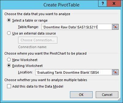
Directed Activity: Create PivotTables and PivotCharts
Objectives
 • Create a PivotTable and PivotChart from Event Frame Data

3.4.1 Comparing Downtime Events Based on Reason Code

We would like to determine which causes of events are the most frequent and costly.
To do this, we will create a PivotChart report from Event Frames generated in AF.
After completing the Event Frame search in the previous section, use the following
instructions to create the Pivot Chart and Pivot Table.
 Step 1 : Go to the Evaluating Tank Downtime Blank sheet, select the Insert ribbon and select
 the PivotChart option. Select the columns and rows of interest from the Downtime
 Raw Data tab. This will create a PivotTable and a PivotChart.

 Step 2 : As input for the PivotTable select the
 cell range in the Downtime Raw Data
 sheet where the CompareEvents
 function has returned the data
 (including the header line).
 Then choose to place the PivotTable
 and PivotChart in the Evaluating Tank
 Downtime Blank sheet.

Tip: if you want to correct the source area later in
time, select all cells of your PivotTable (or choose
the Analyze ribbon), then from the Analyze
Ribbon, select Change Data Source.

 17 | P a g e

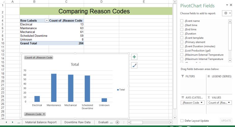
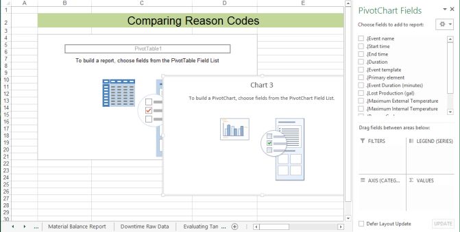
Step 3 : The PivotChart field list should now be shown in your Excel worksheet and a range
 of the worksheet should be designated where the pivot table will be located, as
 shown below.

 Step 4 : Select the PivotTable, and review the PivotTable Field list. These fields come from
 the column names of the Downtime Raw Data sheet.
 Step 5 : To perform a downtime analysis for our Event Frames based on the corresponding
 reason code, select the .|Reason Code line and drag into the Values area. The
 applied Aggregation for the reason codes is COUNT, because these are non-
 numeric values. Select the .|Reason Code line again and drag into the Rows area:

18 | P a g e

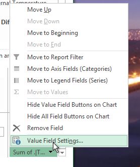
Step 6 : Select the .|Lost Production (gal) line and drag into the Values area. The
 aggregation applied for these numeric values is SUM. Select the .|Temperature
 Difference line and drag into the Values area. Change the aggregation type to
 Average.
 Your PIVOT table is extended 2 additional columns, which summarize corresponding
 production losses and temperature differences, based on the reason codes:

Tip1: if the PivotTable Fields pane was closed and you want to have it available again, select a
cell of your PivotTable. From the right-mouse button menu, select Show Field List.

Tip2: to change the aggregation that is applied to your data, select the dropdown icon on the
field, and choose Value Field Settings… to select another aggregation type.

 19 | P a g e

Step 7 : Let’s enhance our Pivot table for analysis depending on
 individual tank selections.
 Which column of our data represents a tank?
 ______________________________________
 Step 8 : Select a cell in the Pivot Table, and select the Analyze ribbon
 from the Pivot Table tools. Click on Insert Slicer, select
 .|Primary Element and click on OK.

 Step 9 : Add a slicer for the primary element, which allows you to select
 any combination of one or more tanks for our analysis.
 Check various combinations (use Shift- and Ctrl-key for
 selections in the slicer):
 a. all tanks
 b. Mixing Tank1 only
 c. all Mixing Tanks

The PivotTable and the PivotChart will update to show you what reason code is
causing most of the downtime events. In the screenshot above, during the observed
period of time, Electrical and Unknown events were the least common sources of
downtime.

20 | P a g e

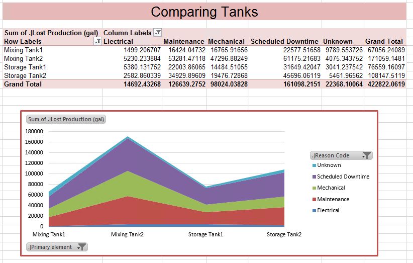
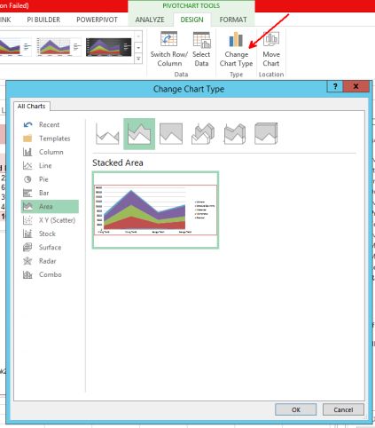
3.4.2 Comparing Downtime Events Based on Tank

Now that we have determined which downtime causes are most frequent, we need to determine
which tank should get our attention first.
 Step 1 : To create a report to compare downtime events based on tanks, we will follow a
 similar procedure as above. Repeat the procedure outlined in Steps 1-4 above to
 create a new PivotChart and PivotTable with the same Event Frame data.
 Step 2 : To perform a downtime analysis for our Event Frames based on the corresponding
 tank, select the .|Lost Production (gal) line and drag into the Values area. The
 applied Aggregation for the reason codes should be SUM. Select the .|Primary
 element line again and drag into the Rows area
 Step 3 : To add an additional visual, drag the .|Reason Code to the Legend (Series) area.

 Step 4 : Select the PivotChart, then go to the Design tab and choose Change Chart Type.
 Choose the Area category on the left, then choose Stacked Area as the Chart Type.

 21 | P a g e

The result is a report that shows us which tank has had the most production loss, along with a
quick glimpse of which reason codes are causing the production loss.

22 | P a g e

Analyze Downtime Events Using PivotTables and PivotCharts
Objectives
 • Analyze Event Frames retrieved from PI DataLink using PivotCharts and PivotTables

Problem Description
The operations manager needs a report that shows which downtime reason is most prevalent
and a comparison showing which tanks are the most problematic. He also would like to see
information about the total production loss from the tanks.
Now that you have imported event data into Excel and created PivotTables and PivotCharts,
use them to analyze the data.
Approach
 Step 1 : You will use the template provided in sheets Downtime Raw Data and Evaluating
 Tank Downtime of the file PI_DataLink-Exercises.xlsx.
 Step 2 : Open the Evaluating Tank Downtime sheet.
 Step 3 : Select the PivotTable under Comparing Reason Codes, then, from the Analyze tab,
 select Refresh

 Step 4 : Select the PivotTable under Comparing Tanks, then, from the Analyze tab, select
 Refresh
 Step 5 : Which Reason Code caused the most production loss overall?
 __________________
 Step 6 : Which Reason Code caused the most production loss for the Storage tanks?
 __________________
 Step 7 : Which Tank has caused the most production loss? __________________

 23 | P a g e

Bonus: Making Reports More User-Friendly
Objective
 o Leverage out-of-the-box Excel functionality to make your report easier to use.

Problem Description
You would like to put some finishing touches on your workbook so that it is easier for others to
use.

Approach
 Step 1 : Hide the sheet containing raw data.
 Step 2 : Configure the PivotTables to automatically refresh data when the workbook is
 opened. (As a result, the PivotCharts will automatically refresh as well).
 Step 3 : Prevent column widths and cell formatting from adjusting on data refresh so the
 PivotCharts will print consistently.

24 | P a g e

Solutions
Analyze Downtime Events Using PivotTables and PivotCharts
 1. Which Reason Code caused the most production loss overall? Use the Comparing
 Tanks PivotTable. Find the reason code corresponding to the highest individual value in
 the Grand Total row (H10:L10).
 2. Which Reason Code caused the most production loss for the Storage tanks? Use
 the Row Labels filter to choose only the storage tanks, then find the reason code
 corresponding to the highest individual value in the Grand Total row.
 3. Which Tank has caused the most production loss? Make sure all tanks are selected
 in the filter for the Comparing Tanks PivotTable, then look at which tank has the highest
 sum of .|LostProduction (gal) in the PivotChart.

Bonus
 1. Right-click the Downtime Raw Data sheet and select Hide
 2. Select the PivotTable, then go to Tools > Analyze > PivotTable > Options > Data >
 Refresh data when opening file (Microsoft doc)

 • Or VBA, although we recommend using out of the box functionality instead if
 possible. Example: when source data changes via Excel Campus
 3. PivotTable Tools > Analyze > PivotTable > Options > Layout & Format > check Autofit
 column widths on update and Preserve cell formatting on update (Microsoft doc)

 25 | P a g e

4. EXERCISE: Improve Performance of Large
 Workbooks

 Objectives
 • Prevent Excel from recalculating when you don’t want it to
 • Use Microsoft’s built-in Inquire add-in to create a summary of what a large
 workbook contains
 • Measure how many data calls PI DataLink makes in the background when
 opening a workbook or recalculating
 • Use Excel’s Formula Auditing tools to see relationships between formulas
 • Improve performance of large workbooks by substantially reducing the
 number of calls PI DataLink must make

 Background
Under the hood, PI DataLink takes the information entered into the task pane for a
given function and creates an AF SDK call. So the more PI DataLink functions you
have, the more AF SDK calls must be made to retrieve data. Thus, it is important to
keep in mind how you can minimize calls when building out or modifying large
workbooks containing many hundreds of formulas (or more).
This section will teach you some best practices when troubleshooting why
workbooks containing many PI DataLink functions open or recalculate slowly. You
will learn how to minimize unnecessary recalculations (each of which could take
minutes); quantify the number of calls made by PI DataLink to its data access layer,
the AF SDK; and finally, reduce the number of calls necessary by using cell ranges
as input and/or bulk data retrieval methods.
For more detailed information on architecture and data flow, see PI DataLink’s
playbook in the Customer Portal. For your convenience, here is the data flow section:
Data Flow
PI System data is retrieved by PI DataLink into Excel in the following manner:
 1. User inputs parameters via the function pane
 2. Recalculation is initiated via OK/Apply or right-click > Recalculate (Resize)
 Function
 3. PI DataLink takes the input parameters and forms an AF SDK call
 4. AF SDK handles reaching out to back-end resources (PI Data Archive, AF
 Server) and calculations
 5. AF SDK returns values to PI DataLink
 6. PI DataLink creates output appropriate for Excel and pastes values into the
 worksheet

26 | P a g e

Directed Activity: Measure AF SDK calls made in the background
Objective
 • Measure how many data calls PI DataLink makes in the background when
 opening a workbook or recalculating

Problem Description
How do you quantitatively measure the background activity to recalculate the PI
DataLink functions in this workbook? Specifically, how do you log the calls PI
DataLink makes to its data access layer, the AF SDK, to retrieve PI System data?

Approach
 Step 1 : Open Excel
 Step 2 : Open the Task Manager (right-click the task bar, or Ctrl+Shift+Esc)
 Step 3 : Right-click on Microsoft Excel (32 bit) and Go to details
 Step 4 : What is the process ID (PID) for the highlighted EXCEL.EXE process? Write it down.
 Note: if you do not have a PID column, add it by right-clicking a column header >
 Select columns.

 Step 5 : Open Windows Explorer and go to %pihome64%\AF. (On the lab machine, this is
 equivalent to C:\Program Files\PIPC\AF)
 Step 6 : Launch AFGetTrace.exe.
 Step 7 : Configure the tracing settings: Enable Whitelist and enter Excel’s PID in the
 Process IDs field
 Step 8 : Verify Enable PI, Enable AF, and Log Headers are all checked
 Step 9 : Select Server and Data keywords

 27 | P a g e

Step 10 : Enable Log and name your log/select log location

 Step 11 : Press the green, triangular Play button
 Step 12 : Open Performance Exercise.xlsx
 Step 13 : Notice the delay in opening as the workbook recalculates. Excel estimates its Commented [JR1]: The delay should be small but still
 recalculation progress in the bottom right: noticeable,

Step 23 : Review the three traces you just generated:
 -when opening the workbook in the default Automatic calculation mode
 -when opening the workbook in Manual calculation mode
 -and when making any change to the workbook
Step 24 : Which trace is empty?
Step 25 : To determine the exact number of AF SDK calls made for a particular action, use the
 AFGetTrace log and Notepad++’s Find All in Current Document functionality.
Step 26 : For example, clear the AFGettrace log output

Step 27 : Perform an action that you saw results in AF SDK calls, such as loading the
 workbook or making a change while in Automatic mode.
Step 28 : Stop the trace (red square).
Step 29 : Open the log in Notepad++
Step 30 : Highlight “End Call Sequence” and press Ctrl+F to open the Find window with those
 search terms auto-filled
Step 31 : Select Find All in Current Document

 29 | P a g e

Step 32 : See how many call sequences exist in the log

 Step 33 : Calculate the total recalculation time by subtracting the first Begin Call Sequence
 time from the last End Call Sequence time
 Step 34 : Calculate the average call sequence time. A relatively fast baseline is about 3-4
 milliseconds per call.
 Step 35 : How many calls are made when opening the workbook in the default Automatic
 mode? How much total time does this data access layer activity take?
 Step 36 : How many calls are made when making any change to the workbook? How much
 total time does it take?

30 | P a g e

Directed Activity: Gather information about the workbook
Objective
 • Prevent Excel from recalculating when you don’t want it to
 • Use Excel’s Formula Auditing tools to see relationships between formulas
 • Use Microsoft’s built-in Inquire add-in to create a summary of what a large
 workbook contains

Problem Description
The operators for a plant your company recently acquired have been using a
workbook for a long time, designed by someone who left or retired years ago. It has
been kind of slow for a long time, but it’s finally gotten so bad they are now asking
you to fix it. You’ve never seen this workbook before. How do you analyze the
workbook to find out a likely root cause?

Approach
 Step 1 : Open Performance Exercise.xlsx
 Step 2 : Select the upper left cell in the block of PIAdvCalcVal functions (C2).
 Step 3 : In the Ribbon, select Formulas > Formula Auditing > Trace Precedents
 Step 4 : Arrows point to the referenced cells containing the data item (B2), start time (C2),
 and end time (D2):

 Step 5 : Notice each date cell in row 1 depends on the cell to the right, such as D1
 referencing E1.
 Step 6 : Remove Arrows and select the right-most date cell (M1).
 Step 7 : Select Trace Dependents. Notice the huge number of arrows generated:

 Clicking Trace Dependents additional times will show successive dependents,
 eventually going all the way to column C. This is a visual reference of how the entire

 31 | P a g e

block of PI DataLink calls is influenced by this one date cell with a formula of
 TODAY(). We will discuss the performance impact of this function in the next
 exercise.
 Step 8 : Switching gears, read Microsoft’s article for more broad coverage of their Inquire
 add-in than will be presented in this lab.
 Step 9 : Go to File > Options > Add-ins > Manage: COM Add-ins and press Go…
 Step 10 : Check Inquire and press OK. An Inquire tab should load in the Ribbon.
 Step 11 : Select Workbook Analysis. If prompted, do not save changes.
 Step 12 : In the Items pane, check Summary, Workbook, and Formulas, then press Excel
 Export…
 Step 13 : Save the analysis, then press Load Export File.
 Step 14 : How many formulas, number of formulas with errors, and hidden/very hidden sheets
 are in this workbook? Commented [JR2]: Inquire is useful for giving you an
 overview of the workbook’s contents and for spotting
 ‘gotchas’, such as hidden sheets you were not aware of.

32 | P a g e

Improve performance by reducing the number of background calls
Objective
 • Improve performance of large workbooks by reducing the number of calls PI
 DataLink must make
 • Learn about volatile functions in Excel recalculation
 • Learn which Excel and PI DataLink functions are volatile

Problem Description
Now that you know this workbook is making a large amount of relatively fast data
calls, how can you help performance by reducing the number of calls?

Read the Volatile and Non-Volatile Functions section of Microsoft’s Excel
Recalculation article. This is also discussed in certain OSIsoft KB articles, such as
After upgrading Microsoft Office, opening complex spreadsheets using PI DataLink is
much slower.
After reading, you should be aware of which Excel functions are volatile. The only PI
DataLink function that is volatile by default is Current Value. Why?
Insert a column into the workbook that contains the current value for each data item.
Do so in such a way that only one call sequence is made to populate the current
values.
Bonus: verify only one call sequence is made using AFGetTrace.

Approach
 Step 1 : Open Performance Exercise.xlsx
 Step 2 : Select cell M1 containing the volatile formula, TODAY()
 Step 3 : Type today’s date or press Ctrl+;
 Step 4 : Using AFGetTrace, observe that AF SDK calls no longer occur when making an
 unrelated change to the workbook, such as typing “test” in cell N3
 Step 5 : To recalculate the entire block of PI DataLink formulas, go to PI DataLink >
 Resources > Settings and select Full calculate, 0s Interval for the Automatic
 Update. Then click the green Update button.
 Step 6 : Using AFGetTrace, observe 1000 AF SDK calls are made for each recalculation
 cycle.
 Step 7 : Click Update again to turn auto-update off.
 Step 8 : Select cell C2 and notice the formula references a single data item, $B2:
 {=PIAdvCalcVal('Raw Data'!$B2,'Raw Data'!C$1,'Raw Data'!D$1,"average (time-
 weighted)","time-weighted",0,1,0,"")}
 Step 9 : Right-click the cell and select Recalculate (Resize) Function (or use the task pane
 > OK)

 33 | P a g e

Step 10 : Notice how the entire row recalculated, not just that single cell, and the formula now
 shows the contiguous range of data items ($B$2:$B$101) instead of the single data
 item.
 Step 11 : Repeat for each column so that there are ten formula arrays, each referencing 100
 data items, instead of 1000 individual formula arrays.
 Step 12 : Turn Update back on
 Step 13 : Using AFGetTrace, observe the number of AF SDK calls has been reduced by an
 order of magnitude. This is because these formulas now meet the conditions under
 which PI DataLink is able to take advantage of bulk AF SDK calls, as documented in
 the user guide’s Retrieval of large amounts of data topic.

34 | P a g e

Solutions
Directed Activity: Measure AF SDK calls made in the background
 1. Calculate the average call sequence time. Total time / # calls = time/call. So 3.8/1000
 = 0.0038s, or 3.8 milliseconds.
 2. How many calls are made when opening the workbook in the default Automatic
 mode? Should be 1000.
 3. How much total time does this data access layer activity take? Should be around 3-
 4 seconds. During testing, it took 3.8s.
 4. How many calls are made when making any change to the workbook? How much
 total time does it take? # of calls and time should be very similar to the open, as the
 functions all being volatile results in all of them recalculating on change, just like they do
 on workbook open.
 5. Which trace is empty? The one covering workbook open when in Manual calculation
 mode should be empty.
Directed Activity: Gather information about the workbook
 1. How many formulas, number of formulas with errors, and hidden/very hidden
 sheets are in this workbook? Use the Inquire report you just generated. Example:

 35 | P a g e

5. EXERCISE: Excel’s New Dynamic Array Functions

 Objectives
 • Learn about Excel’s new dynamic array functions
 • Create a report using PI DataLink and these new Excel functions
 • Brainstorm other ways these functions could prove useful to you

 Background
Microsoft has recently made changes to Excel’s calculation engine that enable
“dynamic arrays”, which allow you to write one formula and return many values. As of
January 17th, dynamic arrays and the new functions that leverage them are available
in all Office 365 channels except Semi-Annual.
In this exercise, we will go through Microsoft’s preview of dynamic arrays. Then, we
will see a few ways these new functions could be used with PI DataLink functions.
Note: In most cases, there are other ways to accomplish the same tasks besides
these new functions, such as VLOOKUP or INDEX(MATCH()). However, the new
functions will generally be simpler and easier to use.

36 | P a g e

Learn about Excel’s new dynamic array functions
Objective
 • Get hands-on experience with dynamic array formulas

Problem Description
Microsoft’s Preview of Dynamic Arrays in Excel describes several aspects of
dynamic arrays and lists multiple dynamic array functions. Read through this article
and the articles on specific functions, such as SORT and FILTER. In addition, read
the article on the XLOOKUP function. Then follow along in the workbook.

Approach
 Step 1 : Open PI_DataLink-Exercises.xlsx to the Dynamic Functions sheet.
 Step 2 : Sort the names in column A with a single dynamic function.
 Step 3 : Notice a couple of new behaviors for dynamic functions—first, when you select any
 cell in the resulting array, the entire array is outlined in blue. In addition, only the top
 left cell in the dynamic array is editable; all other cells in the array have greyed-out
 formulas, and if you attempt to edit the cell, the formula disappears.

 Step 4 : Cleanse the list of names in column D of duplicates with a single dynamic function.
 Step 5 : Filter the list of names in column G by the diet preferences in column H with a single
 dynamic function.
 Step 6 : With a single function, look up the country code for Brazil from the data in columns
 P and R.
 Step 7 : Bonus: Which aspects of this new functionality will work in earlier versions of Excel?
 What will not work?

 37 | P a g e

Use dynamic array functions to complement PI DataLink functions
Objective
 • Use dynamic array functions with PI DataLink functions to derive more value
 out of your data
 • Brainstorm other ways these functions could prove useful to you

Problem Description
You want to enhance your production summaries by sorting production days below a
certain threshold by their total production. After hearing about new dynamic
functions, you think they could be used to quickly accomplish your goals.

Approach
 Step 1 : Go to the Production Summaries sheet
 Step 2 : Use the SORT and FILTER functions to display a list of the days below 200,000
 gallons of total production from the Daily Calculations table, in ascending order.
 Step 3 : Go to the Downtime Raw Data sheet
 Step 4 : In column T, use Compressed Data to retrieve values from yesterday for the tag
 CDM158.
 Note: you will need to enter ‘CDM158 for the data item; otherwise, it will be
 recognized as a reference to the cell CDM158.
 Step 5 : Use the UNIQUE function to retrieve (1) the unique digital states in yesterday’s data
 for CDM158 and (2) the unique reason codes in the event frame data.
 Bonus: Sort the digital states and reason codes alphabetically.

38 | P a g e

Solutions
Learn about Excel’s new dynamic array functions
 1. Open PI_DataLink-Exercises.xlsx to the Dynamic Functions sheet.
 2. In cell B5, use the SORT function and select the range of names: =SORT(A5:A11)
 3. In cell E5, use the UNIQUE function and select the range of names:
 =UNIQUE(D5:D14)
 4. Cell E9 contains a period, which prevents the dynamic array from spilling into the full
 cell range it requires. This results in a #SPILL error. Delete this period, and the
 UNIQUE formula will auto-populate.
 5. In cell U4, use the XLOOKUP function with a lookup value of T4, a lookup array of
 P4:P13, and a return array of R4:R13. If it’s hard to keep track of the different fields,
 use Formulas > Insert Function. =XLOOKUP(T4,P4:P13,R4:R13)
 6. Bonus: It’s probably wise to avoid using dynamic array functionality until your IT
 department rolls out an O365 update containing dynamic arrays to you/your users.
 Dynamic arrays will be converted to legacy Ctrl+Shift+Enter (CSE) formulas in older
 versions of Excel and still work, but dynamic array functions will not be recognized,
 resulting in #NAME? errors.

 Remember that if you need to verify compatibility across multiple Office versions, you
 can use File > Info > Check for Issues > Check Compatibility. For more
 information, read Dynamic array formulas in non-dynamic aware Excel and Dynamic
 array formulas vs. legacy CSE array formulas.
 Use dynamic array functions to complement PI DataLink functions
 1. On the Production Summaries sheet, in cells G20:I20, label columns Criterion, Day,
 and Production Total.
 2. Enter 200,000 into cell G21
 3. In cell H21, filter the Daily Calculations range containing the start time and
 Production Total (gal) by the criterion: =FILTER(A21:B27,B21:B27

7. Similarly, in cell Q8, use the UNIQUE function with the values in the .|Reason Code
 column: =SORT(UNIQUE(L8:L36),,1)

40 | P a g e

6. EXERCISE: Introduction to PI DataLink
 Documentation

 Objective
 • Learn about key articles in OSIsoft Technical Support’s Knowledge Base for
 PI DataLink

 Background
PI DataLink has been and continues to be one of OSIsoft’s most-used client tools.
Over the past two decades, OSIsoft Technical Support has answered well over
100,000 calls concerning PI DataLink. As you might expect, we have created
documentation along the way to help us efficiently answer these calls and deflect
some questions outright as customers can find what they need in our Customer
Portal without our assistance.

This section will give you an overview of the most-used articles for PI DataLink so
that the next time you have a question about PI DataLink the user guide doesn’t
answer, you will know how to find the same resources we use!

 41 | P a g e

Access PI DataLink’s user guide in context
Objective
 • Access the PI DataLink user guide in the context of your current task
 • Understand the structure of the PI DataLink user guide

Problem Description
PI DataLink does not appear in the Ribbon, and you wish to search and view OSIsoft
Knowledge Base articles to help you troubleshoot.

Approach
 Step 1 : You will use the template provided in sheet Operational Start Up of the file
 PI_DataLink-Exercises.xlsx.
 Step 2 : Select a cell containing a PI DataLink function, such as cell A11, and the task pane
 will appear. Commented [JR3]: The task pane will automatically show
 up if “Disable automatic task pane display on click” is
 Step 3 : Select any field in the Compressed Data task pane and press F1 unchecked in DL Settings. The pane appearing is the default
 behavior.
 Step 4 : Alternatively, in the top right of the task pane, click the question mark.
 Commented [JR4]: If the focus is anywhere other than
 Step 5 : This brings up the Compressed Data function topic in the local PI DataLink User the DL task pane, F1 will launch Excel’s help instead of ours
 Guide, which describes each possible input for the function Commented [JR5]: When DL is installed, it puts the user
 guide in %pihome%\help\en\PIDataLink.chm
 Step 6 : Navigate down a level to the Compressed Data example topic. (Each PI DataLink
 function topic has an example.)
 Step 7 : You can also use the function reference for more formula-focused help. Return to
 cell A11 and view the formula.
 Step 8 : In the user guide, navigate to the Function reference topic, select the group
 matching the Ribbon group for your function, then select the exact function. For
 example, Function reference > Multiple-value functions > PICompDat() for
 Compressed Data in cell A11
 Step 9 : Go to the Downtime Raw Data sheet and view the documentation for the Compare
 Events function Commented [JR6]: Compare/Explore Events are the most
 complicated functions PI DataLink offers

42 | P a g e

Directed Activity: Access the Customer Portal
Objective
 • Configure your account (if necessary)
 • Access the Customer Portal

Problem Description
PI DataLink does not appear in the Ribbon, and you wish to search and view OSIsoft
Knowledge Base articles to help you troubleshoot.

Approach
 Step 1 : Go to https://customers.osisoft.com and log in with your OSIsoft single sign-on Commented [JR7]: If lab attendees can’t get in, suggest
 (SSO) account they simply follow along with you and set up their account
 later

 If you do not have an SSO account or have not been added to a site, at
 your convenience go to https://explore.osisoft.com/myosisoft-customer-
 Tip portal/how-to-get-a-login and follow the step-by-step instructions there.

 Step 2 : In the top search bar, search for “datalink playbook” Commented [JR8]: Talking points:

 Step 3 : Click on Playbook – PI DataLink -Product playbooks are the go-to resource for our PSEs who
 answer customer calls. This tip applies to any of our
 Step 4 : In the Troubleshooting section under the Runtime list, select “PI DataLink or PI products—whenever I’m troubleshooting a product, I search
 Builder does not appear in the Ribbon in Excel” “[product name] playbook” to see if one exists
 -Version history, summary of the product’s use case and
 Step 5 : Instead of using the playbook, now access the same article via direct search. Search architecture
 for your issue to find the article, filtering by the KB Articles content type if -Guided troubleshooting steps
 -Links to articles covering common issues
 necessary.
 -Good way to see which parts of the user guide are
 Step 6 : Pretend two months have passed, and you vaguely remember something about an referenced most, ex. DL’s bulk calls section in LiveLibrary
 -Highlight admin task articles, as those are particularly well
 AF tracing utility you used in a PI World lab. You think it could be useful to covered for DL
 troubleshoot your current situation but can’t recall exactly how to use it. Search to
 find an article describing how to use the utility. Commented [JR9]: Demonstrate searching for the ribbon
 issue with different phrasing:

 “datalink not in ribbon”
 “datalink does not show up”
 “datalink does not appear”
 “datalink missing”

 Search early, search often is a KCS technique. No need to
 actually mention KCS, but that’s effectively what we’re
 teaching here
 Commented [JR10]: How do I use the AFGetTrace utility?

 43 | P a g e

44 | P a g e

© Copyright 2020
 OSIsoft, LLC