Buffered Count-Min Sketch on SSD: Theory and Experiments - DROPS
←
→
Page content transcription
If your browser does not render page correctly, please read the page content below
Buffered Count-Min Sketch on SSD: Theory and
Experiments
Mayank Goswami
Queens College, City University of New York
mayank.goswami@qc.cuny.edu

Dzejla Medjedovic
International University of Sarajevo
dzmedjedovic@ius.edu.ba

Emina Mekic
Sarajevo School of Science and Technology
emina.mekic@stu.ssst.edu.ba

Prashant Pandey
Stony Brook University, New York
ppandey@cs.stonybrook.edu

      Abstract
Frequency estimation data structures such as the count-min sketch (CMS) have found numer-
ous applications in databases, networking, computational biology and other domains. Many
applications that use the count-min sketch process massive and rapidly evolving data sets. For
data-intensive applications that aim to keep the overestimate error low, the count-min sketch
becomes too large to store in available RAM and may have to migrate to external storage (e.g.,
SSD.) Due to the random-read/write nature of hash operations of the count-min sketch, simply
placing it on SSD stifles the performance of time-critical applications, requiring about 4-6 random
reads/writes to SSD per estimate (lookup) and update (insert) operation.
     In this paper, we expand on the preliminary idea of the buffered count-min sketch (BCMS)
[Eydi et al., 2017], an SSD variant of the count-min sketch, that uses hash localization to scale
efficiently out of RAM while keeping the total error bounded. We describe the design and
implementation of the buffered count-min sketch, and empirically show that our implementation
achieves 3.7×-4.7× speedup on update and 4.3× speedup on estimate operations compared to
the traditional count-min sketch on SSD.
     Our design also offers an asymptotic improvement in the external-memory model over the
original data structure: r random I/Os are reduced to 1 I/O for the estimate operation. For a
data structure that uses k blocks on SSD, w as the word/counter size, r as the number of rows,
M as the number of bits in the main memory, our data structure uses kwr/M amortized I/Os
for updates, or, if kwr/M > 1, 1 I/O in the worst case. In typical scenarios, kwr/M is much
smaller than 1. This is in contrast to O(r) I/Os incurred for each update in the original data
structure.
     Lastly, we mathematically show that for the buffered count-min sketch, the error rate does
not substantially degrade over the traditional count-min sketch. Specifically, we prove that for
any query q, our data structure provides the guarantee: Pr[Error(q) ≥ n(1 + o(1))] ≤ δ + o(1),
which, up to o(1) terms, is the same guarantee as that of a traditional count-min sketch.

2012 ACM Subject Classification Theory of computation → Data structures and algorithms
for data management, Theory of computation → Streaming models, Theory of computation →
Database query processing and optimization (theory)

Keywords and phrases Streaming model, Count-min sketch, Counting, Frequency, External
memory, I/O efficiency, Bloom filter, Counting filter, Quotient filter
            © Mayank Goswami, Dzejla Medjedovic, Emina Mekic, and Prashant Pandey;
            licensed under Creative Commons License CC-BY
26th Annual European Symposium on Algorithms (ESA 2018).
Editors: Yossi Azar, Hannah Bast, and Grzegorz Herman; Article No. 41; pp. 41:1–41:15
                   Leibniz International Proceedings in Informatics
                   Schloss Dagstuhl – Leibniz-Zentrum für Informatik, Dagstuhl Publishing, Germany
41:2 Buffered Count-Min Sketch on SSD: Theory and Experiments
Digital Object Identifier 10.4230/LIPIcs.ESA.2018.41
Acknowledgements We gratefully acknowledge support from CNS 1408695, CCF 1439084, IIS
1247726, CCF 1725543, SPX, CCF 1716252, CCF 1617618, CNS-1755615, CCF 1755791, and
from Sandia National Laboratories.
1 Introduction
Applications that generate and process massive data streams are becoming pervasive [3, 18,
19, 14, 25] across many domains in computer science. Common examples of streaming data
sets include financial markets, telecommunications, IP traffic, sensor networks, textual data,
etc [3, 10, 26, 7]. Processing fast-evolving and massive data sets poses a challenge to traditional
database systems, where commonly the application stores all data and subsequently does
queries on it. In the streaming model [3], the data set is too large to be completely stored
in the available memory, so every item is seen and processed once — an algorithm in this
model performs only one scan of data, and uses sublinear local space.
The streaming scenario exhibits some limitations on the types of problems we can solve
with such strict time and space constraints. A classic example is the heavy hitter problem
HH(k) on the stream of pairs (at , ct ), where at is the item identifier, and ct is the count of
the item at timeslot t, with the goal of reporting all items whose frequency is at least n/k,
PT
n = t=1 ct . The general version of the problem with the exception of when k is a small
constant1 , can not be exactly solved in the streaming model [22, 26], but the approximate
version of the problem, -HH(k), where all items of the frequency at least n/k − n are
reported, and an item with larger error might be reported with small probability δ, is
efficiently solved with the count-min sketch [11] data structure. The count-min sketch
accomplishes this in O(ln(1/δ)/) space, usually far below linear space in most applications.
The count-min sketch [11] has been extensively used to answer heavy hitters, top k
queries and other popularity measure queries, the central problems in the streaming context,
where we are interested in extracting the essence from an impractically large amount of data.
Common applications include displaying the list of bestselling items, the most clicked-on
websites, the hottest queries on the search engine, most frequently occurring words in a large
text, and so on [24, 19, 27].
The count-min sketch (CMS) is a hashing-based, probabilistic, and lossy representation
of a multiset, that is used to answer the count of an item a (number of times a appears in a
stream). It has two error parameters: 1) , which controls the overestimation error, and 2) δ,
which controls the failure probability of the algorithm. The CMS provides the guarantee
that the estimation error for any item a is more than n with probability at most δ. If we
set r = ln(1/δ) and c = e/, the CMS is implemented using r hash functions as a 2D array
of dimensions r · c.
When and δ are constants, the total overestimate grows proportionately with n, the
size of the count-min sketch remains small, and the data structure easily fits in smaller and
faster levels of memory. For some applications, however, the allowed estimation error of n
is too high when is fixed. Consider an example of n = 230 , where δ = 0.01 and = 2−26 ,
hence the overestimate is 16, and the total data structure size of 3.36GB, provided each
counter uses 4 bytes. However, if we double the data set size, then the total overestimate
also doubles to 32 if stays the same. On the other hand, if we want to maintain the fixed
overestimate of 16, then the data structure size doubles to 6.72GB.
1
When k ≈ 2 this problem goes by the name of majority element.M. Goswami, D. Medjedovic, E. Mekic, and P. Pandey 41:3
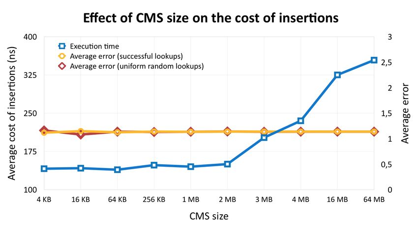
Figure 1 The effect of increasing the count-min sketch size on the update operation cost in RAM.
In this paper, we expand on the preliminary idea of the buffered count-min sketch
(BCMS) [13], an SSD variant of the traditional count-min sketch data structure, that scales
efficiently to large data sets while keeping the total error bounded. Our work expands on the
previous work by introducing a detailed design, implementation, and experiments, as well as
mathematical analysis of the new data structure (our original paper [13], which, to the best
of our knowledge is the only attempt thus far to scale the count-min sketch to SSD, contains
only the outline of the data structure). Our analysis is performed in the external-memory
model [1], which emphasizes the cost of I/O operations over CPU computation. In the
external-memory model, the unit cost is a block transfer of size B between the disk of infinite
size and the main memory of size M (for most input sizes N , M41:4 Buffered Count-Min Sketch on SSD: Theory and Experiments
1.1 Results
1. We describe the design and implementation of the buffered count-min sketch, and
empirically show that our implementation achieves 3.7 × −4.7× the speedup on update
and 4.3× speedup on estimate operations.
2. Our design also offers an asymptotic improvement in the external-memory model [1]
over the original data structure: O(r) random I/Os are reduced to 1 I/O for estimate.
For a data structure that uses k blocks on SSD, w as the word/counter size, r as the
number of rows, M as the number of bits in main memory, our data structure uses
kwr/M amortized I/Os for updates, or, if kwr/M > 1, 1 I/O in the worst case. In typical
scenarios, kwr/MM. Goswami, D. Medjedovic, E. Mekic, and P. Pandey 41:5
blowup in space. The count-sketch can be advisable where the smaller is desired, however,
that would require a much larger data structure. Also, the count-min sketch is more widely
used and applicable and this is why we choose to analyze its SSD performance. One can also
hypothesize that extensions of the count-sketch to disk would benefit from the same hash
localization and buffering techniques as did the count-min sketch given their almost identical
structure.
2.1 External-Memory Model
We use the external-memory model or disk-acces machine (DAM) model [1] to analyze the
on-SSD performance of our data structure. DAM model captures the essential feature of
modern computers, where the CPU computation is orders-of-magnitude cheaper than moving
data between different levels of memory. This deems the cost of I/O transfers the main
bottleneck in many data-intensive applications. In the DAM model, memory is made up of
two levels, main memory of size M and disk of infinite size, and data is transferred between
the two levels using blocks of size B, where usually M = Θ(B 2 ). Once data is in the memory,
all computations are free, and the performance is measured solely by the number of disk
transfers performed. Even though the DAM model only shows the communication between
RAM and disk, it is a useful analogy for any two levels of memory where one is small and fast
and the other one is large and slow (i.e., different cache levels). Therefore, the problem size
need not be that large for the I/O effects to kick in and the DAM model to be applicable.
2.2 Count-Min Sketch: Preliminaries
In the streaming model, we are given a stream A of pairs (ai , ci ), where ai denotes the item
identifier (e.g., IP address, stock ID, product ID), and ci denotes the count of the item. Each
pair Xi = (ai , ci ) is an item within a stream of length T , and the goal is to record total sum
of frequencies for each particular item ai .
For a given estimation error rate and failure probability δ, define r = ln(1/δ) and
c = e/. The count-min sketch is represented via a 2D matrix with c buckets (columns),
r rows, implemented using r hash functions (one hash function per row). CMS has two
operations: UPDATE(ai ) and ESTIMATE(ai ), the respective equivalents of insert and lookup,
and they are performed as follows:
1. UPDATE(ai ) inserts the pair by computing r hash functions on ai and incrementing
appropriate slots determined by the hashes by the quantity ci . That is, for each hash
function hj , 1 ≤ j ≤ r, we set CM S[j][hj (ai )] = CM S[j][hj (ai )] + ci . Note that in this
paper, we use ci = 1, so every time an item is updated, it is just incremented by 1.
2. ESTIMATE(ai ) reports the frequency of ai which can be an overestimate of the true
frequency. It does so by calculating r hashes and taking the minimum of the values found
in appropriate cells. In other words, we return min1≤j≤r (CM S[j][hj (ai )]). Because
different elements can hash to the same cells, the count-min sketch can return the
overestimated (never underestimated) value of the count, but in order for this to happen,
a collision needs to occur in each row. The estimation error is bounded; the data structure
guarantees that for any particular item, the error is within the range n, with probability
at least 1 − δ, i.e., P r[Error(q) ≥ n] ≤ δ.
ESA 201841:6 Buffered Count-Min Sketch on SSD: Theory and Experiments
3 Buffered Count-Min Sketch
In this section, we describe the buffered count-min sketch, an adaptation of the count-min
sketch to SSD. The traditional CMS, when placed on external storage, exhibits performance
issues due to random-write nature of hashing. Each update operation in the CMS requires
r = ln(1/δ) writes to different rows and columns of the CMS. On a large data structure, these
writes become destined to different pages on disk, causing the update to perform O(ln(1/δ))
random SSD page writes. For high-precision CMSs, where δ = 0.001% − 0.01%, this can be
between 5-7 writes to SSD, which is unacceptable in a high-throughput scenario.
To solve this problem, we implement, analyze, and empirically test the data structure
presented in [13] that outlines three adaptations to the original data structure:
1. Partitioning the CMS into pages and column-first layout: We logically divide the CMS on
SSD into pages of block size B. CMS with r rows, c columns, cell size w, and a total of
S = cr w-bit counters, contains k pages P1 , P2 , P3 , . . . , Pk , where k = S/B and each page
spans contiguous B/r columns 2 : Pi spans columns [B(i − 1)/r + 1, Bi/r]. To improve
cache-efficiency, the CMS is laid out on disk in column-first order which allows each
logical page to be laid out sequentially in memory. Thus, each read/write of a logical
page requires at most 2 I/Os.
2. Hash localization: We direct all hashes of an element to a single logical page in the CMS.
The page is determined by an additional hash function h0 : [1, k]. The subsequent r hash
functions map to the columns inside the corresponding logical page, i.e., the range of
h1 , h2 , . . . , hr for an element e is [B(h0 (e) − 1)/r + 1, Bh0 (e)/r]. This way, we direct all
updates and reads related to an element to one logical page.
3. Buffering: When an update operation occurs, the hashes produced for an element are
first stored inside an in-memory buffer. The buffer is partitioned into sub-buffers of
equal size S1 , S2 , . . . , Sk , and they directly correspond to logical pages on disk in that
Si stores the hashes for updates destined for page Pi . Each element first hashes using
h0 , which determines in which sub-buffer the hashes will be temporarily stored for this
element. Once the sub-buffer Si becomes full, we read the page Pi from the CMS, apply
all updates destined for that page, and write it back to disk. The capacity of a sub-buffer
is M/k hashes, which is equivalent to M/kwr elements so the cost of an update becomes
kwr/MM. Goswami, D. Medjedovic, E. Mekic, and P. Pandey 41:7
Algorithm 1 Buffered Count-Min Sketch - UPDATE function.
1 Require : key , r
2 subbufferIndex i := murmur 0 ( key );
3 for i :=1 to r do
4 hashes [ i ] := murmur i ( key );
5 end for
6 AppendToBuffer ( hashes , subbufferIndex );
7
8 if isSubbufferFull ( subbufferIndex ) then
9 bcmsBlock := readDiskPage ( subbufferIndex );
10 for each entry in Subbuffer [ subbufferIndex ] do
11 for each index in entry do
12 pageStart := calculatePageStart ( subbufferIndex );
13 offset := pageStart + entry [ index ];
14 bcmsBlock [ offset ][ index ]++;
15 end for
16 end for
17 w ri t eB cm s Pa g eB ac k To D is k ( bcmsBlock );
18 clearBuffer ( subbufferIndex );
19 end if
Algorithm 2 Buffered Count-Min Sketch - ESTIMATE function.
1 Require : key , k
2 subbufferIndex i := murmur 0 ( key );
3 pageStart := calculatePageStart ( subbufferIndex );
4 bcmsBlock := readDiskPage ( subbufferIndex );
5
6 if i sSubbufferNotEmpty ( subbufferIndex ) then
7 for each entry in Subbuffer [ subbufferIndex ] do
8 for each index in entry do
9 offset := pageStart + entry [ index ];
10 bcmsBlock [ offset ][ index ]++;
11 end for
12 end for
13 clearBuffer ( subbufferIndex );
14 end if
15
16 for i :=1 to k do
17 value := murmur i ( key );
18 offset := pageStart + value ;
19 estimation := bcmsBlock [ offset ][ i - 1];
20 estimates [ i ] := estimation ;
21 end for
22 w r i t e B cm s Pa g eB ac k To D is k ( bcmsBlock );
23 return min ( estimates )
ESA 201841:8 Buffered Count-Min Sketch on SSD: Theory and Experiments
Figure 2 UPDATE operation in the buffered count-min sketch. In-RAM buffer is divided into
sub-buffers and when a sub-buffer is full all updates are flushed to the corresponding page on disk.
r = ln(1/δ) and c = e/. The traditional count-min sketch uses S = cr = (e/) ln(1/δ)
counters/words of space. Recall that for our purposes, 1/n ≤ (n) 1, in one I/O worst case.
2. Let Error(q) = ESTIMATE(q) - TrueFrequency(q). Then for any C ≥ 1,
p
P r[Error(q) ≥ n(1 + (2(C + 1)k log k)/n)] ≤ δ + O((B/e)C ).
p
Remark: By Assumption 1, (2(C + 1)k log k)/n is o(1) (in fact, it is o(1/ log k)). By
Assumption 2, (B/e)C is o(1). Thus we claim that the buffered count-min-sketch gives
almost the same guarantees as a traditional count-min sketch, while obtaining a factor r
speedup in queries. The guarantee for estimates taking 1 I/O is apparent from construction,
as only one block needs to be loaded3 .
The proof is a combination of the classical analysis of CMS and the maximum load of
balls in bins when the number of bins is much smaller than the number of balls. Also, note
that unlike the traditional CMS, the errors for a query q in different rows are no longer
independent (in fact, they are positively correlated: a high error in one row implies more
elements were hashed by h0 to the same bucket as q).
3
In practice, we may need 2 I/Os due to block-page alignment, but never more than 2.M. Goswami, D. Medjedovic, E. Mekic, and P. Pandey 41:9
The hash function h0 maps into k buckets, each having size B (and so we will also call
them blocks). Each bucket can be thought of as a r × B/r matrix. Note that r = ln(1/δ),
and B/r = e/(k). We assume that h0 is a perfectly random hash function, and, abusing
notation, identify a bucket/block with a bin, where h0 assigns elements (balls) to one of the
k buckets (bins).
In this scenario we use Lemma 2(b) from [21] and adapt it to our setting.
I Lemma 2. (Lemma 2(b) from [21]) Let B(n, p) denote a Binomial distribution with
t−np
parameters n and p, and q = 1 − p. If t = np + o((pqn)2/3 ) and x := √ pqn tends to infinity,
then
2
/2−log x− 12 log π+o(1)
P r[B(n, p) ≥ t] = e−x .
Let M (n, k) denote the maximum number of elements that fall into a bucket, when
hashed by h0 .
q
I Lemma 3. Let C ≥ 1 and t = n/k + 2(C + 1) n log k
k . Then
P r[M (n, k) ≤ t] ≥ 1 − 1/k C .
Proof. We first check that t satisfies the conditions of Lemma 2. Since h0 is uniform, p = 1/k
(i.e., each bucket
q is equally probable), and np = n/k. We need to check that the extra
term in t, 2(C + 1) n log
k
k
is o((n(1 − 1/k)/k)2/3 ). This is precisely the condition that
n = ω(k(log k)3 ) (Assumption 1).
Next we apply Lemma 2. In our case,
s
2(C + 1)n log k/k p
x= = 2(C + 1) log k(1 + 1/k − 1),
n(1 − 1/k)/k
Now by assumption 2, (n) goes to zero as n goes to infinity, and so k ∝ 1/(n) goes to
infinity, and therefore x goes to infinity as n goes to infinity. Thus we have that the number
of elements in any particular bucket (which follows a B(n, 1/k) distribution)
q is larger than t
2 2
/2−log x− 12 log π+o(1)
with probability e−x ≤ e−x /2
. Putting in x = 2(C + 1) log k(1 + 1
k−1 ),
we get x2 /2 = (C + 1) log k(1 + 1/(k − 1) ≥ (C + 1) log k, and thus the probability is at most
e−(C+1) log k = 1/k C+1 .
Thus the probability that the maximum number of balls in a bin is more than t is bounded
(by the union bound) by k ∗ (1/k)C+1 = (1/k)C , and the lemma is proved. J
Now that we know that with probability as least 1 − 1/k C , no bucket has more than t
elements, we observe that a bucket serves as a “mini” CMS for the elements that hash to
it. In other words, let n(q) be the number of elements that hash to the same bucket as q
under h0 . The expected error in the ith row of the mini-CMS for q (the entry for which is
contained inside the bucket of q), is E[Errori (q)] = n(q)/(B/r) = n(q)k/e.
By Markov’s inequality Pr[Error
p i (q) ≥ n(q)k] ≤ 1/e. p
Let α = tk/e = (n/k + (2(C + 1)n log k)/k)k/e = (n/e)(1 + (2(C + 1)k log k)/n).
We now compute the bound on the final error (after taking the min) as follows.
P r(Error(q) ≥ eα) = P r(Errori (q) ≥ eα ∀i ∈ {1, · · · , r})
= P r(Errori (q) ≥ eα ∀i| n(q) ≤ t)P r(n(q) ≤ t)
+ P r(Errori (q) ≥ eα ∀i| n(q) ≥ t)P r(n(q) ≥ t)
r C
≤ (1/e) + (1/k)
= δ + 1/k C ,
ESA 201841:10 Buffered Count-Min Sketch on SSD: Theory and Experiments
where the second last equality follows from Markov’s inequality on Errori (q) and Lemma 3.
Finally, by observing that for a fixed δ, k = O(e/B), the proof of the theorem is complete.
5 Evaluation
In this section, we evaluate our implementation of the buffered count-min sketch. We compare
the buffered count-min sketch against the (traditional) count-min sketch. We evaluate each
data structure on two fundamental operations, update and estimate. We evaluate estimate
operation for a set of elements chosen uniformly at random.
In our evaluation, we address the following questions about how the performance of the
buffered count-min sketch compares to the count-min sketch:
1. How does the update throughput in the buffered count-min sketch compare to the
count-min sketch on SSD?
2. How does the estimate throughput in the buffered count-min sketch compare to the
count-min sketch on SSD?
3. What is the effect of hash localization in the buffered count-min sketch on the frequency
overestimate compared to the frequency overestimate in the count-min sketch?
4. What is the effect of changing the RAM-size-to-sketch-size ratio on the update and
estimate performance?
5.1 Experimental setup
To answer the above questions, we evaluate the performance of the buffered count-min sketch
and the (traditional) count-min sketch on SSD by scaling the sketch out of RAM. For SSD
benchmarks, we use four different RAM-size-to-sketch-size ratios: 2, 4, 8, and 16. The
RAM-size-to-sketch-size ratio is the ratio of the size of the available RAM and the size of the
sketch on SSD. To do this, we fix the size of the available RAM to ≈ 64MB and increase the
sketch size to manipulate the ratio. Note that even though 64MB is a rather modest RAM
size, we are primarily interested in observing the changes in performance when the ratio
between RAM and sketch on SSD changes — it is this ratio that determines the frequency
of flushing, and results on a 64MB RAM size should extend to any other RAM/SSD sizes,
if the ratio is preserved. The page size in all our benchmarks was set to 4096B. In all the
benchmarks, we measure the throughput (operations per second) to evaluate the update and
estimate performance.
To measure the update throughput, we first calculate the number of elements we can insert
in the sketch using calculations described in Section 5.2. During an update operation, we
generate 64-bit integers online from a uniform-random distribution using the pseudo-random
number generator in C++. This way, we do not use any extra memory to store the set of
integers to be added to the sketch. We then measure the total time taken to update the
given set of elements in the sketch. Note that for the buffered count-min sketch, we make
sure to flush all the remaining updates from the buffer to the sketch on SSD after the last
update and include the time to do that in the total time.
To measure the estimate throughput, we query for the estimate of elements drawn from a
uniform-random distribution and measure the throughput. The workload in the estimate
benchmark simulates a real-world query workload where some elements may not be present
in the sketch and the estimate operation will terminate early thereby requiring fewer I/Os.
For all the estimate benchmarks, we first perform the update benchmark and write the
sketch to SSD. After the update benchmark, we flush all caches (page cache, directory entries,
and inodes). We then map the sketch into RAM and perform estimate queries on the sketch.M. Goswami, D. Medjedovic, E. Mekic, and P. Pandey 41:11
Table 1 Size, width, and depth of the sketch and the number of elements inserted in count-
min sketch and buffered count-min sketch in our benchmarks (update, estimate, and overestimate
calculation).
Size Width Depth #elements
128MB 3355444 5 9875188
256MB 6710887 5 19750377
512MB 13421773 5 39500754
1GB 26843546 5 79001508
This way we make sure that the sketch is not already cached in kernel caches from the update
benchmark.
We compare the overestimates in the buffered count-min sketch and count-min sketch for
all the four sketch sizes for which we perform update and estimate benchmarks. To measure
the overestimates, we first perform the update benchmark. However, during the update
benchmark, we also store each inserted element in a multiset. Once updates are done, we
iterate over the multiset and query for the estimate of each element in the multiset. We then
take the difference of the count returned from the sketch and the actual count of the element
to calculate the overestimate.
For SSD-based experiments, we allocate space for the sketch by mmap-ing it to a file on
SSD. We then control the available RAM to the benchmarking process using cgroups. We
fix the RAM size for all the experiments to be ≈ 67MB. We then increase the size of the
sketch based on the RAM-size-to-sketch-size ratio of the particular experiment. For the
buffered count-min sketch, we use all the available RAM as the buffer. Paging is handled
by the operating system based on the disk accesses. The point of these experiments is to
evaluate the I/O efficiency of sketch operations.
All benchmarks were performed on a 64-bit Ubuntu 16.04 running Linux kernel 4.4.0-
98-generic. The machine has Intel Skylake CPU U (Core(TM) i7-6700HQ CPU @ 2.60GHz
with 4 cores and 6MB L3 cache) with 32 GB RAM and 1TB Toshiba SSD.
5.2 Configuring the sketch
In our benchmarks, we take as input δ, overestimate O (= n), and the size of the sketch S
as configuration parameters. The depth of the sketch D is dln 1δ e. The number of cells C is
S/CELL_SIZE. And width of the sketch is de/e.
Given these parameters, we calculate the number of elements n to be inserted in the
sketch as C×O
D×e . In all our experiments, we fix δ to 0.01 and maximum overestimate to 8
and change the sketch size. Table 1 shows dimensions of the sketch and number of elements
inserted based on the size of the sketch.
5.3 Update Performance
Figure 3 shows the update throughput of the count-min sketch and buffered count-min sketch
with changing RAM-size-to-sketch-size ratios. The buffered count-min sketch is 3.7×–4.7×
faster compared to the count-min sketch in terms of update throughput on SSD.
The buffered count-min sketch performs less than one I/O per update operation because
all the hashes for a given element are localized to a single page on SSD. However, in the
count-min sketch the hashes for a given element are spread across the whole sketch. Therefore,
ESA 201841:12 Buffered Count-Min Sketch on SSD: Theory and Experiments
Figure 3 Update throughput of the count-min sketch and buffered count-min sketch with
increasing sizes. The available RAM is fixed to ≈ 64MB. With increasing sketch sizes (on x-axis)
the RAM-size-to-sketch-size is also increasing 2, 4, 8, and 16. (Higher is better.)
Figure 4 Estimate throughput of the count-min sketch and buffered count-min sketch with
increasing sizes. The available RAM is fixed to ≈ 64MB. With increasing sketch sizes (on x-axis)
the RAM-size-to-sketch-size is also increasing 2, 4, 8, and 16. (Higher is better.)
the update throughput of the buffered count-min sketch is 3.7× when the sketch is twice the
size of the RAM. And the difference in the throughput increases as the sketch gets bigger
and RAM size stays the same.
5.4 Estimate Performance
Figure 4 shows the estimate throughput of the count-min sketch and buffered count-min
sketch with changing RAM-size-to-sketch-size ratios. The buffered count-min sketch is ≈ 4.3×
faster compared to the count-min sketch in terms of estimate throughput on SSD.
The buffered count-min sketch performs a single I/O per estimate operation because
all the hashes for a given element are localized to a single page on SSD. In comparison,
count-min sketch may have to perform as many as h I/Os per estimate operation, where h is
the depth of the count-min sketch.M. Goswami, D. Medjedovic, E. Mekic, and P. Pandey 41:13
Figure 5 Maximum overestimate reported by the count-min sketch and buffered count-min sketch
for any inserted element for different sketch sizes. The blue line represents the average overestimate
reported by the count-min sketch and buffered count-min sketch for all the inserted elements. The
average overestimate is same for both the count-min sketch and buffered count-min sketch.
5.5 Overestimates
In Figure 5 we empirically compare overestimates returned by the count-min sketch and
buffered count-min sketch for all the four sketch sizes for which we performed update and
estimate benchmarks. And we found that the average and the maximum overestimate
returned from the count-min sketch and buffered count-min sketch are exactly the same.
This shows that empirically hash localization in the buffered count-min sketch does not have
any major effect on the overestimates.
6 Conclusion
In this paper we implemented and mathematically analyzed the buffered count-min sketch
and empirically showed that our implementation achieves 3.7×–4.7× the speedup on update
(insert) and 4.3× speedup on estimate (lookup) operations. Queries take 1 I/O, which is
optimal in the worst case if not allowed to buffer. However, we do not know whether the
update time is optimal. To the best of our knowledge, no lower bounds on the update time
of such a data structure are known (the only known upper bounds are on space, e.g., in [15]).
We leave the question of deriving update lower bounds and/or a SSD-based data structure
with faster update time for future work.
References
1 Alok Aggarwal and S. Vitter, Jeffrey. The input/output complexity of sorting and related
problems. Commun. ACM, 31(9):1116–1127, 1988. doi:10.1145/48529.48535.
2 Austin Appleby. 32-bit variant of murmurhash3, 2011. URL: https://sites.google.com/
site/murmurhash/.
3 Brian Babcock, Shivnath Babu, Mayur Datar, Rajeev Motwani, and Jennifer Widom. Mod-
els and issues in data stream systems. In Proceedings of the Twenty-first ACM SIGMOD-
SIGACT-SIGART Symposium on Principles of Database Systems, PODS ’02, pages 1–16,
New York, NY, USA, 2002. ACM. doi:10.1145/543613.543615.
4 Michael A. Bender, Martin Farach-Colton, Rob Johnson, Russell Kraner, Bradley C.
Kuszmaul, Dzejla Medjedovic, Pablo Montes, Pradeep Shetty, Richard P. Spillane, and Erez
ESA 201841:14 Buffered Count-Min Sketch on SSD: Theory and Experiments
Zadok. Don’t thrash: How to cache your hash on flash. Proc. VLDB Endow., 5(11):1627–
1637, jul 2012. doi:10.14778/2350229.2350275.
5 Burton H. Bloom. Space/time trade-offs in hash coding with allowable errors. Commun.
ACM, 13(7):422–426, 1970. doi:10.1145/362686.362692.
6 Flavio Bonomi, Michael Mitzenmacher, Rina Panigrahy, Sushil Singh, and George Varghese.
An improved construction for counting bloom filters. In Proceedings of the 14th Conference
on Annual European Symposium - Volume 14, ESA’06, pages 684–695, London, UK, UK,
2006. Springer-Verlag. doi:10.1007/11841036_61.
7 Lee Breslau, Pei Cao, Li Fan, Graham Phillips, and Scott Shenker. Web caching and zipf-
like distributions: Evidence and implications. In INFOCOM ’99. Eighteenth Annual Joint
Conference of the IEEE Computer and Communications Societies, pages 126–134, 1999.
8 Mustafa Canim, George A. Mihaila, Bishwaranjan Bhattacharjee, Christian A. Lang, and
Kenneth A. Ross. Buffered bloom filters on solid state storage. In Rajesh Bordawekar
and Christian A. Lang, editors, ADMS@VLDB, pages 1–8, 2010. URL: http://dblp.
uni-trier.de/db/conf/vldb/adms2010.html#CanimMBLR10.
9 Moses Charikar, Kevin Chen, and Martin Farach-Colton. Finding frequent items in data
streams. In Proceedings of the 29th International Colloquium on Automata, Languages and
Programming, ICALP ’02, pages 693–703, Berlin, Heidelberg, 2002. Springer-Verlag. URL:
http://dl.acm.org/citation.cfm?id=646255.684566.
10 Aiyou Chen, Yu Jin, Jin Cao, and Li Erran Li. Tracking long duration flows in net-
work traffic. In Proceedings of the 29th Conference on Information Communications,
INFOCOM’10, pages 206–210, Piscataway, NJ, USA, 2010. IEEE Press. URL: http:
//dl.acm.org/citation.cfm?id=1833515.1833557.
11 Graham Cormode and S. Muthukrishnan. An improved data stream summary: The count-
min sketch and its applications. J. Algorithms, 55(1):58–75, 2005. doi:10.1016/j.jalgor.
2003.12.001.
12 Biplob Debnath, Sudipta Sengupta, Jin Li, David J. Lilja, and David H. C. Du. Bloom-
flash: Bloom filter on flash-based storage. In Proceedings of the 2011 31st International
Conference on Distributed Computing Systems, ICDCS ’11, pages 635–644, Washington,
DC, USA, 2011. IEEE Computer Society. doi:10.1109/ICDCS.2011.44.
13 Ehsan Eydi, Dzejla Medjedovic, Emina Mekic, and Elmedin Selmanovic. Buffered count-
min sketch. In Mirsad Hadžikadić and Samir Avdaković, editors, Advanced Technologies,
Systems, and Applications II, pages 249–255, Cham, 2018. Springer International Publish-
ing.
14 Mohamed Medhat Gaber, Arkady Zaslavsky, and Shonali Krishnaswamy. Mining data
streams: A review. SIGMOD Rec., 34(2):18–26, 2005. doi:10.1145/1083784.1083789.
15 Sumit Ganguly. Lower bounds on frequency estimation of data streams. In International
Computer Science Symposium in Russia, pages 204–215. Springer, 2008.
16 Michael Gertz, Quinn Hart, Carlos Rueda, Shefali Singhal, and Jie Zhang. A data and query
model for streaming geospatial image data. In Torsten Grust, Hagen Höpfner, Arantza Illar-
ramendi, Stefan Jablonski, Marco Mesiti, Sascha Müller, Paula-Lavinia Patranjan, Kai-Uwe
Sattler, Myra Spiliopoulou, and Jef Wijsen, editors, Current Trends in Database Technology
– EDBT 2006, pages 687–699, Berlin, Heidelberg, 2006. Springer Berlin Heidelberg.
17 Amit Goyal, Jagadeesh Jagarlamudi, Hal Daumé, III, and Suresh Venkatasubramanian.
Sketch techniques for scaling distributional similarity to the web. In Proceedings of the
2010 Workshop on GEometrical Models of Natural Language Semantics, GEMS ’10, pages
51–56, Stroudsburg, PA, USA, 2010. Association for Computational Linguistics. URL:
http://dl.acm.org/citation.cfm?id=1870516.1870524.
18 Gurmeet Singh Manku and Rajeev Motwani. Approximate frequency counts over data
streams. In Proceedings of the 28th International Conference on Very Large Data Bases,M. Goswami, D. Medjedovic, E. Mekic, and P. Pandey 41:15
VLDB ’02, pages 346–357. VLDB Endowment, 2002. URL: http://dl.acm.org/citation.
cfm?id=1287369.1287400.
19 Suman Nath, Phillip B. Gibbons, Srinivasan Seshan, and Zachary R. Anderson. Synopsis
diffusion for robust aggregation in sensor networks. In Proceedings of the 2Nd International
Conference on Embedded Networked Sensor Systems, SenSys ’04, pages 250–262, New York,
NY, USA, 2004. ACM. doi:10.1145/1031495.1031525.
20 Prashant Pandey, Michael A. Bender, Rob Johnson, and Robert Patro. A general-purpose
counting filter: Making every bit count. In Proceedings of the 2017 ACM International
Conference on Management of Data, SIGMOD Conference 2017, Chicago, IL, USA, May
14-19, 2017, pages 775–787, 2017. doi:10.1145/3035918.3035963.
21 Martin Raab and Angelika Steger. “balls into bins”—a simple and tight analysis. Random-
ization and Approximation Techniques in Computer Science, pages 159–170, 1998.
22 Tim Roughgarden and Gregory Valiant. Cs168: The modern algorithmic toolbox lecture
#2: Approximate heavy hitters and the count-min sketch, 2018.
23 Tamás Sarlós, Adrás A. Benczúr, Károly Csalogány, Dániel Fogaras, and Balázs Rácz.
To randomize or not to randomize: Space optimal summaries for hyperlink analysis. In
Proceedings of the 15th International Conference on World Wide Web, WWW ’06, pages
297–306, New York, NY, USA, 2006. ACM. doi:10.1145/1135777.1135823.
24 Stuart Schechter, Cormac Herley, and Michael Mitzenmacher. Popularity is everything: A
new approach to protecting passwords from statistical-guessing attacks. In Proceedings of
the 5th USENIX Conference on Hot Topics in Security, HotSec’10, pages 1–8, Berkeley, CA,
USA, 2010. USENIX Association. URL: http://dl.acm.org/citation.cfm?id=1924931.
1924935.
25 David P. Woodruff. New algorithms for heavy hitters in data streams. CoRR,
abs/1603.01733, 2016. URL: http://arxiv.org/abs/1603.01733, arXiv:1603.01733.
26 Yin Zhang, Sumeet Singh, Subhabrata Sen, Nick Duffield, and Carsten Lund. Online
identification of hierarchical heavy hitters: Algorithms, evaluation, and applications. In
Proceedings of the 4th ACM SIGCOMM Conference on Internet Measurement, IMC ’04,
pages 101–114, New York, NY, USA, 2004. ACM. doi:10.1145/1028788.1028802.
27 Qi (George) Zhao, Mitsunori Ogihara, Haixun Wang, and Jun (Jim) Xu. Finding global
icebergs over distributed data sets. In Proceedings of the Twenty-fifth ACM SIGMOD-
SIGACT-SIGART Symposium on Principles of Database Systems, PODS ’06, pages 298–
307, New York, NY, USA, 2006. ACM. doi:10.1145/1142351.1142394.
ESA 2018You can also read