Treadmill speed control - SEMESTER PROJECT - June 7, 2014 - (BioRob) / EPFL
←
→
Page content transcription
If your browser does not render page correctly, please read the page content below
S EMESTER PROJECT

           Treadmill speed control

                                                 Supervisor:
Author:
                                    Jesse van den Kieboom
Maxime Ameho
                                           Florin Dzeladini

                    June 7, 2014
Summary

Treadmills are common tools in the study of locomotion, both for humans and robots. For rehabilitation
use, automatic speed controller have been implemented generally using mechanical systems tethered
to the subject. These are not suited for use with quadruped or reptilian robots. We tried to devise a
tracking device to control a feedback loop for those robots. We first implemented a control library to
send commands to our ForceLink.nl N-mill from a computer over serial port. This was used to design
an experiment to model the dynamics of the treadmill: markers were set on the belt and tracked using
a camera while the treadmill went through accelerations and decelerations. The speed changes were
shown to fit a sigmoid function with stable parameters. Camera and Kinect sensors were used to track
the subject using the treadmill. Camera tracking failed due to challenges posed by the setup’s constraints.
Kinect tracking used plane subtraction and Point in Polygon algorithm to isolate the subject in the
input data. Depth data was used to compute world coordinates of the subject and pass these on to the
automatic controller. Boundary control, and position control were both put to the test. The latter gave
good results whilst the former caused the treadmill to accelerate and decelerate too sharply.
Contents

1 Speed measurement and treadmill dynamics                                                                       1
  1.1 Introduction . . . . . . . . . . . . . . . . . . . . . . . . . . . . . . . . . . . . . . . . . . . . .     1
  1.2 Methods . . . . . . . . . . . . . . . . . . . . . . . . . . . . . . . . . . . . . . . . . . . . . . .      1
  1.3 Results . . . . . . . . . . . . . . . . . . . . . . . . . . . . . . . . . . . . . . . . . . . . . . . .    5

2 Subject tracking and treadmill response                                                                     12
  2.1 Introduction . . . . . . . . . . . . . . . . . . . . . . . . . . . . . . . . . . . . . . . . . . . . . 12
  2.2 Methods . . . . . . . . . . . . . . . . . . . . . . . . . . . . . . . . . . . . . . . . . . . . . . . 12
  2.3 Results . . . . . . . . . . . . . . . . . . . . . . . . . . . . . . . . . . . . . . . . . . . . . . . . 16

3 Conclusion                                                                                                    21

List of figures                                                                                                  i

List of tables                                                                                                   i

Bibliography                                                                                                    iii

References                                                                                                      iii

                                                        II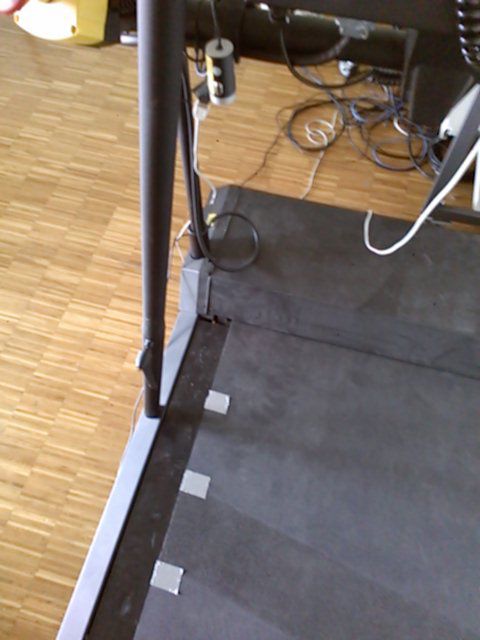
1 Speed measurement and treadmill
     dynamics

1.1 Introduction

The objective of this first part was to design a complete control pattern for the ForceLink.nl treadmill,
meaning implementing a short library to send commands and get status update over the serial port but
also building a model to know how the treadmill responds to these commands and then design them
accordingly. . The second goal spawned from the need to not only respond to the displacement of the
subject on the treadmill, but also respond adequately to get smooth transitions. Sharp changes of speed
could impact the stability of the subject. Moreover one use of the treadmill in our case is the study of
gait under stable conditions, abrupt changes could alter the results such studies. Clearly defining the
behaviour of the treadmill and particularly the dynamics of its acceleration as a reaction to a requested
change in speed, would give us better speed control and possibly a control precision exceeding that of
the native controller. Once a model is established, it can be used to build a response model to subject
displacement. The first step was building a setup to measure to get an external measurement of the
actual speed of the treadmill, as its controller status update only provided the target speed. Markers were
used to get a clear vision of the movement and the displacement was measured using a webcam. Then
remained to fit a working model to the acceleration, which involved determining accurately the phases
in the values recorded and assessing the dependence of acceleration on the starting speed, requested
speed differential and on the actual initial speed.

1.2 Methods

1.2.1 Treadmill

The treadmill we used was a N-Mill by ForceLink.nl of length 225cm and width 120cm. It offers a
command panel with start, stop, speed control, elevation control, and heartbeat measuring. Speed range
is 0.1km · h−1 to 12km · h−1 with 0.1 increment. Elevation goes from 0% to 20%.

1.2.2 Command library

Protocol The protocol was provided by the company and described the messages as series of bytes
composing the data frame with the validation information (Table 1.1a) and the message frame with the
actual data (Table 1.1b).

                                                    1
Figure 1.1: Experimental setup for speed measurement

The two CRC-16 bytes served as integrity check, ensuring the whole data arrived uncorrupted using 16-
bit Cyclic redundancy check (CRC-16; [1]). Status command —get and set — used a structure containing
all the values available to the controller. Sadly the controller had the same precision as the control panel,
and did not offer speed increments lower than 0.1 km · h−1 .

Communication with the treadmill controller required use of the serial port. Instead of implementing this
de novo we used a library1 designed for communication with arduino boards and adapted it to our needs.
Following the same logic as for the signal transmission, we used a simple library2 implementing those
algorithms. The rest of the implementation was quite straightforward: we declared for all common use
operations: Start, stop, setSpeed and setElev plus one to get the Status of the treadmill. The commands
were represented by predefined static arrays of chars, those for start/stop command did not carry data
and were therefore constant, and those for status changes which contained command details such as
speed or elevation (see Table 1.1c). Start/Stop and status commands had constant values and most of
the bytes of the other commands were constant since the addressing didn’t change, the only changes
necessary were the value we wanted to make vary and the CRC integrity checks. To get the other values
that did not vary were checked first against the getStatus command.

1.2.3 Dynamics model

Experimental setup To establish our model we had to get actual speed data. To obtain this, several
methods were envisioned: mainly tracking markers using various devices or coupling the rotation of the
treadmill to a measuring apparatus. In the end we chose to track markers in visual data obtained using a
webcam because of the easy availability of the material required. The trade-off was a lower precision due
to optical artifacts — mainly motion blur — and a lower resolution because of frame rate limitations and
processing. The main parameter for choosing the marker was getting a solid fixation on the treadmill’s
non-skid surface without hindering its functioning. We settled on using gaffer tape squares although it
did not give the best contrast for tracking, because it proved the most resilient. We stuck markers spaced
by 20 centimeters, not too close to avoid blending of the visual data. The webcam was set perpendicular

1   arduino-serial – C code to talk to Arduino, https://github.com/todbot/arduino-serial/
2   On-line CRC calculation and free library: http://www.lammertbies.nl/comm/info/crc-calculation.html

                                                          2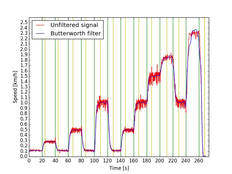
Figure 1.2: Experimental setup for speed measurement

to the treadmill’s plane at a height of about 90 centimeters to get a wide enough field of view and reduce
the need for focus adaptation, on entry and exit of markers (Figures 1.2 1.3a 1.3b).

Data treatment The most basic assumption we made was that the webcam was set appropriately
perpendicular to the ground and therefore the displacement we recorded occurred exclusively in the y
direction. The field of view actually treated was reduced in the x dimension to only record a thin line
making the dimension of the markers mostly irrelevant. Data was then treated using OpenCV. To detect
the marker, the class SimpleBlobDetector was used, which thresholds the image, extracts contours (using
Suzuki’s algorithms [3]) and groups their centers to obtain blobs. We controlled two parameters: color
filtering to mark light blobs and area filtering. The latter was used to ensure correct behaviour in edge
cases — entry and exit — so that cropped markers tracking is discontinued at once. To track blobs we
assumed the displacement was small between two frames, less than 10 pixels, and thus associated in
consecutive frames close detected keypoints. To compute the actual speed, we tried two methods:

Threshold: we first checked time of passage of each blob at a threshold y coordinate: knowing the
     distance between two markers, this allowed to calculate speed. The time resolution was however
     not good enough to work with because of the low speed of the treadmill.

Continuous: To increase the resolution, we kept track of the displacement between each frame. An
     additional step was required to convert the speed in meters per second: we measured the actual
     length of the field of view to get the pixel to meter ratio of the camera: 51.5cmf or350px ⇒ 6.8px/cm
     All time keeping was performed using C++11’s  module, assuming that the delay between
     the camera and the data processing was sufficiently constant.

Experiment series     We chose to build our model based on the two parameters that would be readily
available when actually trying to control the subject positioning:

  1. Difference between current speed and requested speed

  2. Current speed

                                                    3
(a) Field of vision of the camera
(b) Reduced field of view for actual tracking
with y direction
Figure 1.3: Camera input data
4Figure 1.4: Qt graphical interface for treadmill control
Therefore we designed our measures by programmatically sending the treadmill through a sequence
of speed plateaus using the command library. The remote control had the advantage of allowing us to
accurately record the time when the command was sent which proved an asset when processing the
data. The sequence mixed values of our two parameters (Table 1.2)
1.3 Results
Command library The command library worked smoothly, allowing both outbound and inbound
communication. It was complemented with a minimal graphical interface designed with Qt4.81 to control
the treadmill from the computer (Figure 1.4). Although it did not allow for greater precision in speed
control than the actual command panel it granted the possibility to stop the treadmill by setting its speed
to 0.0 km · h−1 rather than stopping it, making the start-up more reactive. The only flaw was a somewhat
unpredictable behaviour when multiple instances running at the same time —for example, monitoring
the status with the GUI while sending commands from the tracking setup— , probably due to conflicting
access to the serial port, leading to unwanted changes in elevation and speed.
Dynamics model The set of data we gathered using the threshold method proved to have too low a
time resolution to be usable to fit a model, and therefore only the continuous measurements were used.
But it was still useful to check the consistency of the second set of results. Indeed figure 1.5 shows that
plateau values are preserved between both methods. This correlation gives credit to the measurement.
However the sharp increase of the shift between measured and displayed speed with the increase of
the requested speed, the root mean square going from 0.012 at 0.1km · h−1 to 0.15 at 2.0km · h−1 (Table
1.3), shows a net corruption of our measures by speed artifacts. Therefore in subsequent experiences
the maximum speed was set to 1.5 km · h−1 because motion blur became too marked at higher speed to
accurately compute speed. Moreover even with this continuous tracking, the sampling rate was limited
by the resolution of the visual data of the camera. Indeed at low speeds, some blobs could register
displacement under one pixel with too high a sampling rate therefore setting their speed to zero. This
had to be taken into account when setting the time resolution. To reduce noise we filtered the data using
1 Qt Project: http://qt-project.org
5Figure 1.5: Comparison of two speed measurement methods: Threshold and Continuous. In green the
speed set in the controller
Butterworth low-pass filter with passband 0-0.2Hz and a 70dB attenuation in the stopband. We then
wanted to define the boundaries of each acceleration phase. Each start was easily given by the time of
issue of the command and we computed the end by calculating the standard deviation over 5 points to
check if the speed was still changing and checking when it got small enough to consider the speed stable
(< 0.001)(Figure 1.6). We then tried to fit a model to our data. Our first intuition was that the speed
followed a first order differential model:
−t
s(t) = startspeed + (f inalspeed − startspeed) ∗ (1 − e τ )
Correlation was good with a coefficient of determination over 0.9 but the shape of the curve was not
perfect (Figure 1.7), we therefore tried adding another parameter and fitting a sigmoid function. We
chose Gompertz function:
−τ2 ·x
s(t) = startspeed + (f inalspeed − startspeed) ∗ e−τ1 ·e
which gave a closer fit, all R2 values over 0.99 (Figure 1.8.
To get more significant results we launched series of measures with repeated change of speed between
the same values to even out noise and artefacts. These performed 40 consecutives accelerations and
decelerations between the same thresholds. 4 series were done: between 0.1 and 0.3 km−1 , 0.1 and 1
km−1 , 0.5 and 1km−1 , 0.5 and 15km−1 .
6Figure 1.6: Raw speed data and filtered data (lowpass 0.2Hz Butterworth) and bounds of acceleration
phase. Green lines mark the time of each speed command. Yellow lines mark the computed
end of acceleration (standard deviation < 0.001)
The value of each parameter stays around the same value. These experiments show some common
artefacts, namely the peak of speed at the time of each commands opposed to the acceleration sent,
which is most likely due to an added blur motion with the sharp change in speed.
7Figure 1.7: First order differential fit on the eight first acceleration phases with coefficient of determination
R2
Figure 1.8: Gompertz function fit on the eight first acceleration phases with coefficient of determination
R2
8Figure 1.9: Value of parameter τ2 for each speed range in order: 0.1-0.3, 0.1-1, 0.5-1, 0.5-15
Figure 1.10: Value of parameter τ2 for each speed range in order: 0.1-0.3, 0.1-1, 0.5-1, 0.5-15
9Identifier Contents
Sync char Identifier of the sender:computer or.controller
DestAdr Identifier of the recipient
Message Frame see table 1.1b
CRC16-1 Validation bit: MSB of CRC-16 of data
CRC16-2 Validation bit: LSB of CRC-16 of data
(a) Data frame of signal
Identifier Contents
MsgID Command sent
LEN0 MSB of length of the data sent
LEN1 LSB of length of the data sent
Data If command needs a value: see table 1.1c
(b) Message frame of signal
Identifier Contents
Status Stopped/Running/Emergency Stopped
Dist Running distance in meters
Speed Current speed in 0.1 km · h−1
Elev Current elevation in %
Elev_analog Analog value from potentiometer
Heatbeat Heartbeat rate
Time Time displayed on panel
Id_key_pressed Last key id pressed
(c) Data structure of signal
Table 1.1: Message breakdown for treadmill communication
10speed [km · h−1 ] time [s]
0.1 0
0.3 20
0.1 40
0.5 60
0.1 80
1.0 100
0.1 120
0.5 140
1.0 160
1.5 180
1.0 200
2.0 220
2.5 240
0.0 260
Table 1.2: Speed command and time of emission
Plateau RMS error
1 0.0216
2 0.0138
3 0.0051
4 0.0147
5 0.0191
6 0.0124
7 0.0086
8 0.0130
9 0.0144
10 0.162
11 0.027
Table 1.3: Root Mean Square error for each plateau. Plateau 1 corresponds to the first 0.3km · h−1
stabilization.
112 Subject tracking and treadmill response
2.1 Introduction
This part contained the gist of the project: detecting the subject on the treadmill and building the feedback
loop to control its position based on visual data. First we searched literature to look for the most adequate
setup to track the user, considering the means at hand and our specific needs. Our first choice used a
webcam but along the way, faced with difficulties in the implementation, we switched to depth detection
using a Kinect. We then had to treat the input to isolate our subject, namely subtract background and
treat for noise. The next challenge was using this input to compute the actual position of the subject,
which was hindered by the positioning of the camera that had to contend with the potential variability
of the shape and dimensions of the subject. The initial goal was to make the recognition and positioning
robust against accidental occurrences, like the operator coming into the detection zone, but time lacked
to make a truly resilient detector, and we had to make do with a simpler system. Once the position was
determined, the only remaining point was to close the loop, and make the treadmill actually react to this
data, using two models, one trying to bind the subject between two limit positions and the other one
trying to keep him at a set position by modulating the speed.
2.2 Methods
2.2.1 Literature research
Treadmills are commonly used in rehabilitation, therefore the speed control is a known problem. However
the common solutions are mostly thought for human subjects. They are often force-based using an
interaction between the user and a mechanical system which cannot be used with most of the existing
robots in our lab, or would require heavy adjustments between each subject [8]. Other methods require
heavy modification of the treadmill and fine control of the environment to measure the position of
the user which is not our goal [9]. The sonar based tracking from [13] would have been usable and
apparently gave good result but was eventually dismissed because of the lower versatility it seemed to
offer, since the sensor and emitter need to be parallel to the treadmill plane which could have been tricky
to implement on some robots such as Pleurobot. Magnetic tracking such as used in [7] were considered
but not used because of their less immediate availability and possible interference with the high amount
of electrical software in the vicinity of the treadmill. Eventually we chose to focus on optical-based
tracking:
Camera: Dismissing user interaction, simple background subtraction should be enough to isolate the
subject for tracking, since the treadmill offers good contrast with its flat black surface. To be robust
12Figure 2.1: Possible positioning of tracking device
against interactions, silhouette lookup could be used ([5]) or more simply color data. Most ordinary
cameras have sufficient frame rate to ensure a good response time. Moreover, if tracking proves
difficult, markers could be used such as LEDs or QRcodes-like devices, the latter presenting the
addition advantage of offering storage for additional data if need be. However a downside is that
cameras reduce the data to two dimensions which can make position estimation more complicated.
Kinect: Using a Kinect sensor would correct the drawback of camera tracking by adding depth informa-
tion. It has good precision in our working range ([12]) and a good linearity which is more important
than precision since absolute positioning is not required. It suffers however from disparity in
the depth measurements on all edges ([11]) which could be a problem depending on the angle of
the sensor. It also has lower frame rate than a webcam, namely around 30FPS, which shouldn’t
however be a problem since this would limit reaction time only around a speed differential of
1.5m · s−1 between the treadmill and the subject.
Positioning of the sensor:
Front: Lower scalability: dependant on robot size and movement pattern. Harder to calibrate in case of
large displacements of the visible part of the subject perpendicular to the treadmill direction. But
easier to use with Kinect or ultrasounds.
Top: Easy to measure displacement for any robot. Con icts with Coman fixation to treadmill frame.
Side: Same weaknesses as front, depending on height. It is not fit for Kinect tracking for robots such as
Pleurobot cause the depth varies with perpendicular movement.
Diagonal: Medium scalability, Distance measurement harder than vertical camera, more dependent
on gait, but doable with known camera angle. Rendered much easier with use of marker (lesser
impact of speci
c robot silhouette on tracking). More likely to
nd a visible
xed point
13Figure 2.2: Experimental setup for Kinect tracking
2.2.2 Camera
The camera was attached at position 4 on the treadmill’s structure. The first step we took towards
isolating the subject was using background subtraction. The goal was to first record a frame of the
treadmill without the subject to use as a basis of comparison for subsequent frames keeping only varying
pixels. We used the OpenCV implementation based on a Mixture of Gaussian (MOG) model ([6]). We
then planned to use feature detection to get significant corners defining our subject. Again OpenCV
offered a convenient interface: the ORB keypoint detector and descriptor extractor combined FAST
algorithm for detection, Harris corner filter for ranking and BRIEF for description ([10]). This step should
offer more security against accidental noise in the input but our focus was getting the information needed
to close the loop and command the treadmill. To track the position of the subject, the features should be
combined to get the centroid, we used a simple mean to this end, while others methods could be more
precise but would decrease the genericity. Problems arose when trying to project the position on the
depth axis of the treadmill: namely differentiating between standing and crawling which can give closely
related images but don’t compute the same way. Indeed the center of gravity for the former would
correspond to a position at about mid-height while in the latter the corresponding point is roughly on
the ground plane in the other case. This made designing a generic response complicated. Moreover
precise calculations would depend on specific characteristics of the camera — field of view, angle of
fixation, distortion — also increasing the specificity.
2.2.3 Kinect
Faced with the issues of tracking with a camera we switched to using Kinect which provided us with an
additional information: depth. The attachment of the sensor proved a bit difficult and we had to settle
with a tripod positioned at the end of the treadmill (Figure 2.2)Interface with the sensor was achieved
using OpenNI framework, however to ease treatment, the data was then converted to be passed to
OpenCV. The input data was displayed in a GLUT windows to allow for user input and give feedback
on the quality of the user extraction. Getting a clear image of the subject went through several steps:
14Plane subtraction: First, we tried to suppress input coming from the treadmill ground plane. To do
this we got 4 reference points on that plane, determined by user input (mouse click), and computed
the resulting plane using cross-product:
With points P0 = (x0 , y0 , z0 ), P1 = (x1 , y1 , z1 ), P2 = (x2 , y2 , z2 ), P3 = (x3 , y3 , z3 )
A normal vector to the plane: n = P0 P1 × P2 P3
A Cartesian equation of plane: n0 x + n1 y + n2 z = n · P0
Subsequently all points with depth greater than this plane were deleted.
Maximum depth: Points further away than the command panel were simply discriminated based on
depth. The coordinates had to be transformed from screen space to world space for this using
a utility function provided by OpenNI which proved to be computationally heavy in earlier
iterations.
Polygonal field of view: To remove data outside the treadmill on both sides we restricted the treated
data to a polygonal field. This was implemented using Ray-casting algorithm to solve the Point-in-
Polygon problem.
All parameters in these treatments were set to be provided by the user at the start of the application
to better adapt to different setups, camera position and such changes. With our input data cleaned up,
we tried to implement tracking of the subject. Our first approach was using the segmentation routines
provided by OpenNI but these relied on Skeleton tracking which did not fit our goals, to track variously
shaped subjects. We thus defaulted to OpenCV feature detection algorithms. The SimpleBlobDetector
did not achieve good results we then turned to the GoodFeatureDectector [4]. This got us back to a
situation similar to what we had using a webcam, but with a more clearly defined subject, less noise, and
an additional information to compute position. To reduce noise, morphological operator (i.e. opening
and closing: [2]) were performed on the image before feature detection. Lack of time drove the following
design choices: no treatment was done to protect the feature detection against occasional noise and
the position of the subject was computed roughly by averaging the position of the features. There is a
vast area of improvement in this field that could be achieved by coupling the feature detection to some
silhouette or skeletal constraint that could be trained for each subject, and k-nearest neighbours could be
applied to segment the data and compute a better average position. Using the average feature position
we would get the corresponding depth value and projected it in world space before using it to compute
the feedback.
2.2.4 Feedback loop
Setting up the basis of the loop was simple enough. Using our command library we set up a Control
class which offered a function receiving a position and forwarding to the treadmill whether it should
accelerate or decelerate. We took two different approaches to motivate that decision-making. The first
one was setting boundaries between which the treadmill would run at constant speed and either increase
or decrease its speed when either of these boundaries was crossed. The second approach stored a target
position and continuously strove to maintain the subject at this position. In both cases we used OpenNI
15Figure 2.3: Background subtraction using MOG
to project in world coordinates. Lack of time made the implementation of the second approach sketchy
but it could be improved by analyzing the evolution of the speed of the subject and harnessing the model
we built for the treadmill dynamics to smoothly curve its position back to equilibrium.
2.3 Results
2.3.1 Camera
MOG background subtraction provided a good outline of the subject but left a lot of noise on the image
(Figure 2.3). Some of it was reduced using morphological operators, but there still remained some
sizeable artefacts. Namely it can be seen in Figure 2.3 that a part of the CoMan is cut off by subtraction.
This is mostly due to reflections on its torso, altering the input values.
Feature detection suffered from this inconsistent subtraction since the corners detected varied heavily
from one frame to the other, rendering registration difficult. Combined with the issue of projecting our
2d data in the three dimensional world coordinate system, this motivated our choice to switch to a Kinect
sensor to make use of the additional depth data to lessen these problems.
2.3.2 Kinect
Subject extraction Plane subtraction gave good results but was sensitive to both point placement and
Kinect placement. Indeed depth values were not exactly linear on the whole range of the sensor, even
less so a as it got parallel to the ground, meaning either the center part of the treadmill appeared despite
the subtraction, or some space above the plane was cut off near the ends of the treadmill (Figure 2.5).
16Figure 2.4: Feature detection using ORB
Figure 2.5: Artefact in plane subtraction, probably caused by distortion of depth data on Kinect detection
edges
17The best solution to this problem was increasing the height of the sensor and inclining it towards the
most horizontal position attainable while keeping all the treadmill in the field of view.
The best placement would thus have been to attach it to the frame of the treadmill directly above the
subject but this would have conflicted with the supporting apparatus of the CoMan robot. This could
be circumvented by using two Kinects positioned at the front and the back, but would require more
computation to correlate the data sent from both sensors. Maximum depth limitation was inconsistent
leaving unpredictable amounts of noise and had to be offset by an empiric bias, this could be left to the
user to tamper with via the interface. Setting the field of view was the easiest way to remove data outside
the treadmill and once trimmed from unnecessary costly copies and operations was quite efficient and
did not alter the frame rate by a significant margin.
Feedback loop Testing was severely limited by time constraints. The averaged feature position was
good enough but there were some inconsistencies in the associated depth that could not be smoothed.
Using boundaries to control the position of the subject did not give good results: the reaction of the
treadmill was too sharp and its acceleration curve not steep enough to react in the distance between the
boundary and either end of the treadmill. Keeping a fixed position gave better results which could be
further improved using the dynamics model designed in the first part. For a start we could compute the
target speed needed to reposition evenly. If a stable speed could be attained by quickly alternating speed
commands, there would also be the possibility of using more precise speeds to adapt to the subject.
18(a) Raw RGB data
(b) Raw Kinect depth data
19(c) Plane subtraction from Kinect depth data
(d) Polygonal field of view from Kinect depth data
Figure 2.6: Kinect data treatment
203 Conclusion
Several stepping stones were set to build a complete automatic speed controller for the treadmill. The
implementation of a library to send commands by serial port was the most basic brick. We then tried
to model its dynamics to give us and future users a better comprehension, and better control over the
speed changes we want to ellicit. We used markers and a camera to get an external measure of the speed
of the treadmill. This setup suffered from the lack of high-speed camera which would have avoided
speed artifacts and motion blur. The acceleration was shown to fit a sigmoid function with parameters
close to constant. These experiments were however limited and could be further developed with a better
sensor, and more systematic parametric search. We chose to use optical input to track the subject on
the treadmill, because the sensors were more readily available to us. Camera tracking was however
too complex to implement due to some of the constraints of our setup, namely we couldn’t attach it
directly at the top of the treadmill to fit CoMan fixation. The diagonal field of view proved a challenge to
project distance values. Kinect was a more interesting choice since the depth data allowed both easier
tracking and easier position computation. Using plane subtraction and PIP algorithm a clear view of
the subject was achieved. Position calculation and treadmill controlled switfly ensued though with
some limitation due to lack of time. It was seen that keeping the subject towards a target position was
more efficient than keeping it between set boundaries. Avenues of improvement are numerous, but
the most interesting concern subject tracking. It can be made both more robust — by using silhouette
extraction,color data from Kinect’s camera, segmentation based on depth — and more precise for position
data by eliminating remaining noise and improving the center of gravity of the subject’s computation,
possibly using k-neighbours’ algorithm.
21List of Figures
1.1 Experimental setup for speed measurement . . . . . . . . . . . . . . . . . . . . . . . . . . . 2
1.2 Experimental setup for speed measurement . . . . . . . . . . . . . . . . . . . . . . . . . . . 3
1.3 Camera input data . . . . . . . . . . . . . . . . . . . . . . . . . . . . . . . . . . . . . . . . . 4
1.4 Qt graphical interface for treadmill control . . . . . . . . . . . . . . . . . . . . . . . . . . . 5
1.5 Comparison of two speed measurement methods: Threshold and Continuous. In green
the speed set in the controller . . . . . . . . . . . . . . . . . . . . . . . . . . . . . . . . . . . 6
1.6 Raw speed data and filtered data (lowpass 0.2Hz Butterworth) and bounds of acceleration
phase. Green lines mark the time of each speed command. Yellow lines mark the computed
end of acceleration (standard deviation < 0.001) . . . . . . . . . . . . . . . . . . . . . . . . 7
1.7 First order differential fit on the eight first acceleration phases with coefficient of determi-
nation R2 . . . . . . . . . . . . . . . . . . . . . . . . . . . . . . . . . . . . . . . . . . . . . . . 8
1.8 Gompertz function fit on the eight first acceleration phases with coefficient of determina-
tion R2 . . . . . . . . . . . . . . . . . . . . . . . . . . . . . . . . . . . . . . . . . . . . . . . . 11
1.9 Value of parameter τ2 for each speed range in order: 0.1-0.3, 0.1-1, 0.5-1, 0.5-15 . . . . . . . 11
1.10 Value of parameter τ2 for each speed range in order: 0.1-0.3, 0.1-1, 0.5-1, 0.5-15 . . . . . . . 11
2.1 Possible positioning of tracking device . . . . . . . . . . . . . . . . . . . . . . . . . . . . . . 13
2.2 Experimental setup for Kinect tracking . . . . . . . . . . . . . . . . . . . . . . . . . . . . . . 14
2.3 Background subtraction using MOG . . . . . . . . . . . . . . . . . . . . . . . . . . . . . . . 16
2.4 Feature detection using ORB . . . . . . . . . . . . . . . . . . . . . . . . . . . . . . . . . . . . 17
2.5 Artefact in plane subtraction, probably caused by distortion of depth data on Kinect
detection edges . . . . . . . . . . . . . . . . . . . . . . . . . . . . . . . . . . . . . . . . . . . 17
2.6 Kinect data treatment . . . . . . . . . . . . . . . . . . . . . . . . . . . . . . . . . . . . . . . . 20
iList of Tables
1.1 Message breakdown for treadmill communication . . . . . . . . . . . . . . . . . . . . . . . 9
1.2 Speed command and time of emission . . . . . . . . . . . . . . . . . . . . . . . . . . . . . . 10
1.3 Root Mean Square error for each plateau. Plateau 1 corresponds to the first 0.3km · h−1
stabilization. . . . . . . . . . . . . . . . . . . . . . . . . . . . . . . . . . . . . . . . . . . . . . 10
iiReferences
[1] W.W. Peterson and D.T. Brown. “Cyclic Codes for Error Detection”. In: Proceedings of the IRE 49.1
(Jan. 1961), pp. 228–235. ISSN: 0096-8390. DOI: 10.1109/JRPROC.1961.287814.
[2] Jean Serra. Image Analysis and Mathematical Morphology. Orlando, FL, USA: Academic Press, Inc.,
1983. ISBN: 0126372403.
[3] Satoshi Suzuki and KeiichiA Be. “Topological structural analysis of digitized binary images by
border following”. In: Computer Vision, Graphics, and Image Processing 30.1 (Apr. 1985), pp. 32–46.
ISSN: 0734189X. DOI: 10.1016/0734-189X(85)90016-7.
[4] J. Shi and C. Tomasi. “Good features to track”. English. In: Proceedings of IEEE Conference on
Computer Vision and Pattern Recognition CVPR-94. IEEE Comput. Soc. Press, 1994, pp. 593–600. ISBN:
0-8186-5825-8. DOI: 10.1109/CVPR.1994.323794.
[5] N.R. Howe. Silhouette Lookup for Automatic Pose Tracking. 2004. DOI: 10.1109/CVPR.2004.164.
[6] Z. Zivkovic. “Improved adaptive Gaussian mixture model for background subtraction”. English.
In: Proceedings of the 17th International Conference on Pattern Recognition, 2004. ICPR 2004. Vol. 2.
IEEE, 2004, 28–31 Vol.2. ISBN: 0-7695-2128-2. DOI: 10.1109/ICPR.2004.1333992. URL: http:
//ieeexplore.ieee.org/articleDetails.jsp?arnumber=1333992.
[7] Lichtenstein et al. A feedback-controlled interface for treadmill locomotion in virtual environments. 2007.
DOI : 10.1145/1227134.1227141.
[8] Joachim Von Zitzewitz, Michael Bernhardt, and Robert Riener. “A novel method for automatic
treadmill speed adaptation”. In: IEEE Transactions on Neural Systems and Rehabilitation Engineering
15.1 (2007), pp. 401–409.
[9] Jeff Feasel et al. “The integrated virtual environment rehabilitation treadmill system”. In: IEEE
Transactions on Neural Systems and Rehabilitation Engineering 19.3 (2011), pp. 290–297.
[10] Ethan Rublee et al. “ORB: An efficient alternative to SIFT or SURF”. English. In: 2011 International
Conference on Computer Vision. IEEE, Nov. 2011, pp. 2564–2571. ISBN: 978-1-4577-1102-2. DOI: 10.
1109/ICCV.2011.6126544. URL: http://ieeexplore.ieee.org/articleDetails.
jsp?arnumber=6126544.
[11] M.R. Andersen et al. Kinect Depth Sensor Evaluation for Computer Vision Applications. ECE-TR 6.
Department of Engineering – Electrical and Computer Engineering, Aarhus University, Feb. 2012.
[12] Kourosh Khoshelham and Sander Oude Elberink. Accuracy and Resolution of Kinect Depth Data for
Indoor Mapping Applications. 2012. DOI: 10.3390/s120201437.
iii[13] Jungwon Yoon, Auralius Manurung, and Irfan Hussain. “Speed Adaptation of a Small Size
Treadmill Using Impedance Control Approach for Rehabilitation”. In: Intelligent Robotics and
Applications. Ed. by Lee et al. Vol. 8102. Lecture Notes in Computer Science. Springer Berlin
Heidelberg, 2013, pp. 165–176. ISBN: 978-3-642-40851-9. DOI: 10.1007/978- 3- 642- 40852-
6_19. URL: http://dx.doi.org/10.1007/978-3-642-40852-6_19.
ivYou can also read