3 Climatology of Ultraviolet Radiation at High Latitudes Derived from Measurements of the National Science Foundation's Ultraviolet Spectral ...
←
→
Page content transcription
If your browser does not render page correctly, please read the page content below
3 Climatology of Ultraviolet Radiation at High
  Latitudes Derived from Measurements of the
  National Science Foundation’s Ultraviolet Spectral
  Irradiance Monitoring Network

        Germar Bernhard, Charles R. Booth, and James C. Ehramjian
                                 5340 Riley Street
                Biospherical Instruments Inc., San Diego, CA, USA
                       E-mail: bernhard@biospherical.com
                         E-mail:booth@biospherical.com
                          E-mail:jime@biospherical.com

 Abstract Solar ultraviolet (UV) radiation has been measured at seven sites
 of the National Science Foundation’s UV Spectral Irradiance Monitoring
 Network (UVSIMN) for up to 20 years. Data are used to establish a UV
 climatology for each site and to quantify differences between sites. Most
 locations are at high latitudes and include the South Pole; two research
 stations at the Antarctic coast (McMurdo and Palmer); the city of Ushuaia at
 the tip of South America; the Arctic village of Barrow; and Summit, a
 research camp established at the top of Greenland’s ice sheet. UV levels at
 San Diego, California were also analyzed as an example of a lower-latitude
 location. The climatologies focus on the UV Index, which was derived from
 measured solar spectra of global irradiance. For each site and day of year,
 the average, median, and maximum UV Index at solar noon, as well as 10th
 and 90th percentile values, were calculated. Measurements were also compared
 with pre-ozone-hole UV levels estimated from historical measurements of
 total ozone. The analysis indicates a large effect of the ozone hole on the
 UV Index at the three Antarctic sites, and to a lesser extent at Ushuaia. UV
 Indices measured at South Pole during the ozone hole period (October and
 November) are 20% − 80% larger than measurements at comparable solar
 elevations during summer months. During October and November, the
 average UV Index between 1991 and 2006 was 55% − 85% larger than the
 estimate for the years 1963 − 1980. The UV Index at McMurdo shows a
 similar asymmetry about the solstice. In October and November, the
 average UV Index is about 30% − 60% higher now than it was historically.
 The largest UV Index ever measured at Palmer was 14.8. This value exceeds
 the maximum UV Index of 12.0 observed at San Diego. While the average
3    Climatology of Ultraviolet Radiation at High Latitudes Derived from Measurements of
      the National Science Foundation’s Ultraviolet Spectral Irradiance Monitoring Network

  UV Index at Ushuaia is fairly symmetrical about the solstice, maximum UV
  Indices as high as 11.5 have occurred in October at times when the ozone
  hole passed over the city. The annual cycle of UV radiation at Barrow is
  governed by large seasonal changes of total ozone, albedo, and cloud cover.
  The UV Index does not exceed 5 due to less severe ozone depletion over the
  Arctic: changes in UV over the last 30 years are on average less than ±8%.
  A comparison of UV levels at network locations reveals that differences
  between sites greatly depend upon the selection of the quantity used for the
  comparison. Average noontime UV Indices at San Diego during summer are
  considerably larger than noontime UV levels under the ozone hole at all
  Antarctic sites. The difference diminishes, however, when daily doses are
  compared because of the effect of 24 hours of sunlight during Antarctic
  summers. Data analysis further revealed that broken clouds at the South
  Pole can enhance spectral UV irradiance at 400 nm by up to 30% above the
  clear-sky value due to multiple reflections between the snow-covered
  surface and the cloud ceiling.
     Keywords     solar ultraviolet radiation, Antarctica, Arctic

3.1     Introduction
When the ozone hole was discovered in 1984 (Chubachi, 1984; Farman et al., 1985),
there was concern about increased levels of ultraviolet radiation in Antarctica.
UV radiation was not measured in Antarctica at that time, prompting the U.S.
National Science Foundation (NSF) to establish a UV monitoring program,
which is now known as the “NSF Ultraviolet Spectral Irradiance Monitoring
Network (UVSIMN)” (Booth et al., 1994). Similar monitoring activities also
commenced in the 1980s and 1990s in Canada (Fioletov et al., 2001), Europe
(e.g., Gröbner et al., 2006), New Zealand (McKenzie et al., 1999), the United
States (Kaye et al., 1999), and other regions. The UVSIMN network currently
consists of six sites at high latitudes and a system at San Diego, California. It has
been operated by Biospherical Instruments Inc. (BSI) since 1988. An overview of
network sites is provided in Table 3.1 and Fig. 3.1. The program employs SUV-100
and SUV-150B spectroradiometers, which measure global spectral irradiance
between 280 nm and 600 nm with a bandpass of about 1.0 nm (SUV-100) or
0.63 nm (SUV-150B) full width at half maximum (FWHM). Results have been used
in about 100 peer-reviewed publications as well as for scientific assessments of
ozone depletion published by the World Meteorological Organization (e.g., WMO,
2007). A complete list of references and additional information about the network
can be found in Operations Reports (e.g., Bernhard et al., 2006a) and at the
project’s website http://www.biospherical.com/NSF.

                                                                                       49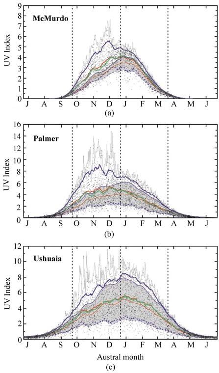
UV Radiation in Global Climate Change: Measurements, Modeling and Effects on Ecosystems

                                  Table 3.1 Network sites

         Site          Latitude Longitude Elevation Established   Used in Study
South Pole, Antarctica 90° 00'S    —       2841 m    Feb 1988 Jan 1991 − Jan 2007
McMurdo, Antarctica 77°    50'S 166° 40'E   183 m    Mar 1988 Dec 1989 − Jan 2007
Palmer, Antarctica     64° 46'S  64°03'W     21 m   May 1988 Mar 1990 − Apr 2006
Ushuaia, Argentina     54° 49'S  68°19'W     25 m    Nov 1988 Nov 1988 − Jun 2005
San Diego, California 32° 46'N 117° 12'W     22 m    Oct 1992 Oct 1992 − Aug 2006
Barrow, Alaska         71°19'N 156° 41'W      8m     Dec 1990 Jan 1991 − Apr 2007
Summit, Greenland      72°35'N   38°27'W 3200 m      Aug 2004 Aug 2004 − Nov 2006

     Figure 3.1 Map of UVSIMN sites (created by Eric Gaba based on a Fuller map).
                                           , ±20°
     Vertical lines indicate latitudes of 0°    , ±40°, and ±60°  . (The Fuller Projection
     Map design is a tradmark of the Buckminster Fuller Institute © 1938, 1967 and 1992.
     All rights reserved, http://www.bfi.org)

   In this chapter, a climatology of UV radiation at UVSIMN sites is presented.
UV radiation at high latitude sites is distinct from conditions at lower latitudes due
to small solar elevations; up to 24 hours of sunlight during spring and summer;
extended periods of darkness during winter; the annually occurring ozone hole
over Antarctica and recent episodes of severe ozone depletion over the Arctic; high
surface albedo from seasonal or year-round snow and ice cover; small influence
of clouds in the interior of Antarctica and Greenland due to low atmospheric
water content; and small aerosol optical depth. Large changes in UV radiation
due to the ozone hole can be expected, although other factors are also important.
However, a confirmation of trends in UV based on measurements of the UVSIMN
remains elusive. By analyzing measurements from South Pole, Palmer, and
McMurdo, Bernhard et al. (2004; 2005; 2006b) concluded that linear trend
estimates are by and large not significant at the 95.5% confidence level. Significant
linear trends were observed only for the months of February and March at
McMurdo (owing to changes in cloudiness and/or albedo), and for February at
Palmer. Several factors contribute to this finding: (1) the network’s operation
started only in the late 1980s after the ozone hole had already been observed;
(2) time-series of about 15 − 18 years are still considered short for reliable trend
detection (Weatherhead et al., 1998); (3) there is a large year-to-year variability
in total ozone, cloudiness, and albedo at most network sites, which obstructs the

50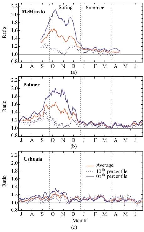
3    Climatology of Ultraviolet Radiation at High Latitudes Derived from Measurements of
      the National Science Foundation’s Ultraviolet Spectral Irradiance Monitoring Network

detection of possible long-term changes; (4) measurement uncertainties affect the
detection of trends; and (5) the stratospheric chlorine loading (and the potential
for ozone depletion) was highest at the turn of the century (WMO, 2007),
approximately in the middle of UVSIMN time-series. The last factor suggests
that changes in UV radiation over the period of UVSIMN operations should be
described with a second-order rather than a linear function. In addition to the
availability of ozone-depleting chemicals, the depth and extent of the ozone hole
is also largely controlled by meteorology, planetary wave activity, and stratospheric
temperatures (Rex et al., 2004; WMO, 2007). These factors show large changes
from year to year. Despite these variabilities, the largest UV intensities at austral
UVSIMN sites were observed in 1997 and 1998 when stratospheric chlorine
concentrations were at their maximum (Bernhard et al., 2004, 2005, 2006b). While
we do not attempt trend estimates in this study, we do estimate past UV levels at
five network sites from historical measurements of total ozone, and contrast these
estimates with the climatology established from recent measurements of the
UVSIMN. This analysis documents large changes in the Antarctic UV climate that
have occurred during the last 40 years.

3.2     Data Analysis

3.2.1     Data

Measurements from all sites with the exception of San Diego are based on
“Version 2 NSF Network Data” (Bernhard et al., 2004), available at
http://www.biospherical.com/NSF/Version2. Version 2 data have been corrected
for the cosine error of the instruments, have a wavelength uncertainty of less than
 ± .04 nm ( ± 1σ), and were normalized to a uniform bandwidth of 1 nm FWHM.
The expanded standard uncertainty of erythemal irradiance (CIE action spectrum
by McKinlay and Diffey, 1987) and spectral irradiance at 400 nm varies between
4.2% and 6.8% (coverage factor 2, equivalent to a confidence level of 95.5%, or
2σ-level). Measurements are complemented with calculations of the radiative
transfer model UVSPEC/libRadtran (Mayer and Kylling, 2005). Measurements
during clear skies agree with model calculations to within ± 5% on average.
More details on Version 2 data and model spectra from South Pole, McMurdo,
Palmer, Barrow, and Summit can be found in publications by Bernhard et al.
(2004, 2005, 2006b, 2007, 2008).
    Version 2 data for San Diego, including model spectra, are not available as of
this writing. Measurements from San Diego are based on the original “Version 0”
data release (Booth et al., 1994; Bernhard et al., 2006a). Data were scaled up by 5%,
which is the typical difference between Version 0 and 2 for erythemal irradiance
observed at the other sites. Version 2 corrections are of less importance for San
                                                                                       51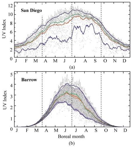
UV Radiation in Global Climate Change: Measurements, Modeling and Effects on Ecosystems

Diego because of the smaller solar zenith angles (SZAs) occurring at this site.
Nevertheless, San Diego data have an additional uncertainty of about 3%.

3.2.2    Establishment of Climatologies

Climatologies discussed in this study are based on measurements near local solar
noon and daily doses. The latter were derived by integrating measurements over
24-hour periods. Spectra were measured hourly until 1997 and quarter-hourly
thereafter. The following times (provided in Universal Time) were associated
with noon: McMurdo: 01:00; Palmer: 16:00; South Pole: 00:00; Ushuaia: 17:00;
San Diego: 20:00; Barrow: 22:00; and Summit: 15:00. To set up a climatology
for noontime irradiance, we calculated for every site and every day of year the
average, median, and maximum, as well as the 10th and 90th percentiles, using
data from the periods indicated in the last column of Table 3.1. As the maximum
may not always occur at noon due to changing clouds and total ozone, we also
calculated the maximum within ± 2 hours ( ± 12 hours for South Pole) of the
times indicated above. This value is denoted “daily maximum.”
   Figure 3.2(a) shows the resulting climatology for the UV Index (i.e., erythemal
irradiance multiplied with 0.4 cm2/μW (WHO, 2002)) at the South Pole. The time-
axis of the plot starts at winter solstice (22 December). Individual measurements
are indicated by small dots. Average and median are plotted as red and green
lines, respectively. Ten percent of the measurements are below (above) the lower
(upper) blue line. The daily maximum is indicated by a thin grey line. All lines
exhibit a large day-to-day variability. To facilitate interpretation, an 11-day running-
average filter was applied to the average, median, and 10th and 90th percentiles.
The resulting graph is plotted in Fig. 3.2(b) and will be discussed further below.

3.2.3    Estimates of Historical UV Indices

Based on historical ozone data and model calculation, the climatology of the UV
Index for years preceding the development of the ozone hole was estimated for
all sites with the exception of San Diego and Summit. The procedure is explained
using South Pole as an example. Historical total ozone data at South Pole are
available from observations of Dobson spectrophotometers performed by the
Global Monitoring Division (GMD) of NOAA’s Earth System Research Laboratory
(ESRL) (Climate Monitoring and Diagnostics Laboratory, 2004). Measurements
started in 1963. Data from 1963 − 1980 were used for estimating past UV levels.
   Year-to-year variability of UV at South Pole is mainly influenced by total
ozone. Variations of surface albedo in the UV and visible wavelength range are
smaller than ± 1% (Grenfell et al., 1994). Except at times following volcanic
eruptions, the aerosol optical depth at 500 nm is typically only 0.012 (Shaw,
52
3 Climatology of Ultraviolet Radiation at High Latitudes Derived from Measurements of
the National Science Foundation’s Ultraviolet Spectral Irradiance Monitoring Network
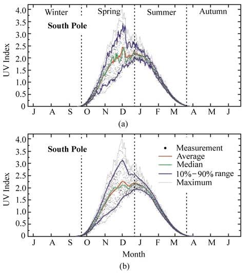
Figure 3.2 Climatology of UV Index at South Pole. Measurements at 00:00 UT
of the years 1991 − 2007 are indicated by black dots. Average and median are plotted
as red and green lines. 10% of the measurements are below (above) the lower (upper)
blue line. The daily maximum is indicated by a thin grey line. The plot starts at the
winter solstice. Summer solstice, and vernal and autumnal equinoxes are indicated
by broken lines. Panel (a): Unsmoothed data. Panel (b): Same data as in (a), but with
an 11-day running-average applied to the average, median, 10% and 90% lines
1982). Attenuation by clouds is small due to the low atmospheric water vapor
content and the moderation of cloud effects by the high ( > 0.96) albedo (Nichol
et al., 2003). By comparing measurements with the clear-sky model, it was
determined that the average attenuation of spectral irradiance at 345 nm is only
6%. Cloud transmission at South Pole has also been determined from measurements
of total irradiance (0.3 μm − 3.0 μm) using pyranometers (Dutton et al., 2004).
Although this study did not indicate a significant linear trend of cloud
transmission between 1976 and 2001, an oscillation on a decadal timescale was
observed with a small downward trend in the late 1970s, followed by an upward
trend between 1982 and 1995, and a downward trend thereafter. The small
relative changes in cloud transmission of about ± 2% reported by Dutton et al.,
(2004) have a very small effect ( < ± 1%) on the UV Index due to the diminished
cloud influence at shorter wavelengths (Bernhard et al., 2004). Based on these
considerations we assumed that all parameters affecting the radiative transfer did
not change during the last 40 years, with the exception of atmospheric ozone
concentrations. The historical clear-sky UV Index for the years 1963 − 1980 was
53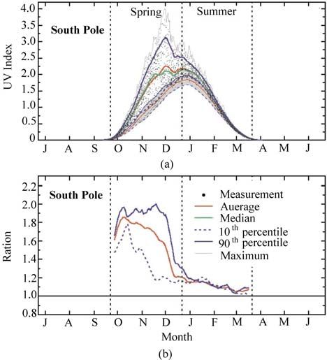
UV Radiation in Global Climate Change: Measurements, Modeling and Effects on Ecosystems

consequently modeled based on the average parameters used for processing
South Pole Version 2 data of the years 1991 − 2007, with the exception of total
ozone which was taken from the GMD Dobson data set.
   The range of historical UV levels for a given day is mostly controlled by
year-to-year changes in total ozone and cloudiness. To account for the variability
introduced by clouds, we integrated measured and modeled spectra from the
years 1991 − 2007 over the wavelength interval 337.5 nm − 342.5 nm, calculated
the ratio of measurement to model, and used the results for estimating cloud-
induced variability in UV intensities. This result was also applied to historical
measurements. This approach assumes that year-to-year cloud-variability did not
change during the last four decades, which is justified considering the small
effect of clouds on UV discussed earlier. We also note that the wavelength interval
of 337.5 nm − 342.5 nm is virtually unaffected by atmospheric ozone concentrations,
and attenuation by clouds has only a weak wavelength dependence between 300 nm
and 340 nm (Seckmeyer et al., 1996). The ratio of measurement to model for the
337.5 nm − 342.5 nm interval is therefore also appropriate for quantifying the
effect of clouds on the UV Index. We estimate that the overall uncertainty in
calculated historical UV Indices due to cloud effects is ± 2%.
   Results of these calculations are shown in Fig. 3.3. The red line is the historical
average UV Index estimated from the average total ozone column of the years
1963 − 1980 measured with the Dobson, and the average attenuation by clouds of
about 6% derived from Version 2 data. Figure 3.3 also includes the estimated 10th
and 90th percentiles from the historical variability of total ozone (thin black lines
in Fig. 3.3) and year-to-year differences in cloud transmission estimated from
recent measurements (broken black lines). The two ranges were combined in
quadrature to estimate the 10th and 90th percentiles for both effects (blue lines).
During summer, variations induced by ozone and clouds are of similar magnitude.
Variations during spring are dominated by ozone.

     Figure 3.3 Estimate of the historical UV Index at South Pole. The red line is the
     average. The ranges defined by the 10th and 90th percentiles caused by variability
     of total ozone and cloud transmission are indicated by thin black and broken black
     lines respectively. The two ranges were combined in quadrature resulting in the
     span indicated by blue lines

54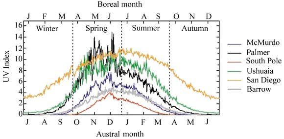
3   Climatology of Ultraviolet Radiation at High Latitudes Derived from Measurements of
     the National Science Foundation’s Ultraviolet Spectral Irradiance Monitoring Network

   A comparison of UV Indices measured during the years 199 − 2007 and UV
Indices modeled for the years 1963 − 1980 is shown in Fig. 3.4(a). An 11-day
moving average was applied to all lines, except the line of the daily maximum.
To better emphasize differences between the two periods, the average, and 10th
and 90th percentiles from the current measurements were ratioed against the
respective data from the historical period. The results are shown in Fig. 3.4(b).
The difference of measurements performed before and after the solstice (22
December) is further highlighted in Fig. 3.5. Data from 21 December were ratioed
against data from 23 December, data from 20 December were ratioed against
data from 24 December, and so forth. If atmospheric conditions had been the same
before and after the solstice, the ratio would be close to unity and only slightly
( < ± 1%) affected by the different Earth-Sun distance before and after the mid-
summer mark. Fig. 3.5 shows that the actual situation is very different. Results
shown in Figs. 3.4 and 3.5 are further discussed below.

     Figure 3.4 Comparison of UV Index measured during the last 17 years with
     historical estimate for South Pole. Panel (a): Individual measurements, average,
     median, range of 10th − 90th percentiles, and daily maximum. Recent measurements
     are indicated by thick lines; historical data are indicated by thin lines and grey-
     shading. Panel (b): Ratio of recent-to-historical data for average, and 10th and 90th
     percentiles

                                                                                             55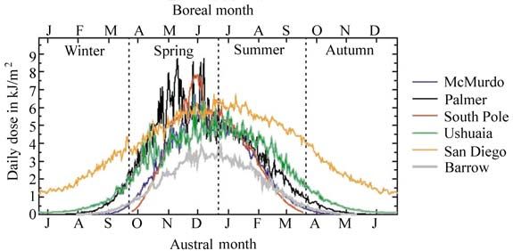
UV Radiation in Global Climate Change: Measurements, Modeling and Effects on Ecosystems

      Figure 3.5 Comparison of the UV Index at the South Pole for periods before and
      after the summer solstice (22-December). Data from 21-December were ratioed
      against data from 23-December, data from 20-December were ratioed against data
      from 24-December, and so forth. Ratios of recent measurements are indicated by
      thick lines; historical data are indicated by thin lines and grey-shading. Red lines
      refer to the average noontime UV Index, broken and solid blue lines to the 10th and
      90th percentiles, respectively. The thin grey line is the ratio for the daily maximum
      of recent data. The broken vertical line indicates the equinox

3.3     UV Index Climatology
A similar analysis as described previously for the South Pole was also performed
for McMurdo, Palmer, Ushuaia, San Diego, and Barrow. The data record for Summit
is still too brief for meaningful interpretation. A description of results for each
site is provided below.

3.3.1     South Pole

The effect of the ozone hole is quite pronounced in measurements from the South
Pole (Figs. 3.4 and 3.5). There is a strong asymmetry between spring and summer.
The daily maximum and 90th percentile peak at the end of November, shortly before
the time when the annual ozone hole typically starts to disintegrate (Fig 3.4(a)).
The maximum UV Index ever observed was 4.0 and was measured on 30
November 1998.
   There is a striking difference between recent measurements and the estimate
for historical data. During October and November, recent measurements from the
years 1991 − 2007 are on average 55% − 85% larger than in the past (red line in
Fig. 3.4(b)). The difference for the 90th percentile is about 95%. Recent data peak
at the end of November, but the peak is absent in the historical estimate. Past UV
Indices for January and February are 10% − 20% lower than contemporary data.
By comparing GMD Dobson total ozone data of the years 1963 − 1980 with data
of the years 1991 − 2005, we found that the increase in UV radiation for these two

56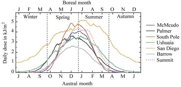
3   Climatology of Ultraviolet Radiation at High Latitudes Derived from Measurements of
     the National Science Foundation’s Ultraviolet Spectral Irradiance Monitoring Network

months can also be attributed to changes in total ozone. Compared to the earlier
period, monthly average total ozone for the years 1991 − 2005 are lower by the
following percentages: January: 12%; February: 7%; October: 48%; November: 35%;
and December: 19%. Differences for all months are statistically significant.
   Figure 3.5 indicates that contemporary measurements taken before the solstice
are larger than UV Indices measured after the mid-summer mark (i.e., ratios are
larger than one). Not surprisingly, the difference increases with the time from the
solstice. On 13 October (70-day mark), the average and 90th percentile are larger
by 82% and 102% respectively, than on the conjugate day of 2 March. Maximum
UV Indices measured on the two days differ by 140% (grey line in Fig. 3.5). This
pattern is very different from the situation prevalent before the development of
the ozone hole. Prior to the 1980s, the reconstructed UV Index was smaller before
the solstice: the thin red line in Fig. 3.5 is smaller than one up to day 50 from the
solstice, and close to one thereafter.
   Figures 3.4(a) and 3.5 also indicate that the 10th percentile is lower in spring
than summer, both for recent and historical data. This characteristic is a consequence
of the natural annual cycle of ozone concentrations caused by the Brewer-
Dobson circulation (Holton et al., 1995). This phenomenon leads to a poleward
transport of ozone from the tropics during the winter and early spring, resulting
in an ozone maximum in spring and a minimum in autumn. During times in the
spring when either the South Pole is outside the perimeter of the ozone hole or
the ozone hole has already closed for the year, total ozone tends to be larger than
in summer. Such situations lead to lower UV Indices in spring relative to summer.
In contrast, when the ozone hole is over the South Pole, ozone concentrations are
smaller than during the summer, explaining the annual cycle of the 90th percentile.

3.3.2    McMurdo Station

McMurdo is affected by the ozone hole from September until early December
(Fig. 3.6(a)). The maximum UV Index was 7.6 and occurred in November; UV
Indices measured after the solstice were below 5.5. The 90th percentile also exhibits
a distinct maximum in late November. The average UV Index is fairly symmetric
within ± 40 days about the solstice, but the 10th percentile is lower in the spring
than in the summer. This feature is again a consequence of the Brewer- Dobson
circulation. Historical UV Indices for McMurdo were estimated from total ozone
measured by TOMS on NASA’s Nimbus-7 satellite (McPeters and Labow, 1996).
Measurements began in 1978, when the ozone hole had already started to develop.
Model calculations were based on the average ozone column measured between
1978 and 1981. The UV irradiance derived from this calculation is therefore likely
already larger than UV intensities prevailing in the 1960s. Due to the short
reference period, it was not possible to calculate a range of historical UV Indices

                                                                                      57
UV Radiation in Global Climate Change: Measurements, Modeling and Effects on Ecosystems
caused by variations in ozone during the pre-ozone-hole period. The grey range
in Fig. 3.6(a) reflects variation by cloudiness only. Cloud effects are considerably
larger compared to the South Pole due to optically thicker clouds at the Antarctic
coast and lower surface albedo, ranging from 0.84 during winter and early spring
to about 0.74 in summer (Bernhard et al., 2006b). Contemporary measurements
are significantly above the historical estimate for all months. Figure 3.7(a) shows
that the average UV Index for October and November is 30% − 60% larger now
than it was historically. The 90th percentile is higher by 70% − 110%. The increase
in the ratio of contemporary to historical data during September reflects the
gradual photochemical loss in stratospheric ozone concentrations as the ozone
Figure 3.6 Same as Fig. 3.4(a), but for McMurdo (Panel (a)), Palmer (Panel (b)),
and Ushuaia (Panel (c))
583 Climatology of Ultraviolet Radiation at High Latitudes Derived from Measurements of
the National Science Foundation’s Ultraviolet Spectral Irradiance Monitoring Network
Figure 3.7 Same as Fig. 3.4(b), but for McMurdo (Panel (a)), Palmer (Panel (b)),
and Ushuaia (Panel (c))
hole forms at the end of winter. For January through March, differences are on
the order of 8% − 15%. Increased UV levels for these months are a consequence
of lower total ozone values during the 1980s and 1990s, also observed for months
not directly affected by the ozone hole (WMO, 2007). Approximately the same
increase in the UV Index of 5% − 15% was observed at all austral network sites
during summer months (compare Figs. 3.4(b) and 3.7(a), (b), (c)).
3.3.3 Palmer Station
The patterns of measured and historical UV Indices at Palmer are similar to those
at McMurdo, but the magnitudes are different. The highest UV Index occurs in
59UV Radiation in Global Climate Change: Measurements, Modeling and Effects on Ecosystems
spring, reaching a maximum of 14.8. The 90th percentile is considerably enhanced
during spring. Particularly large UV-B levels were observed in November and
early December during years when the polar vortex became unstable and air
masses with low ozone concentration moved toward the Antarctic Peninsula. In
combination with the relatively high solar elevations in those months, it led to
UV intensities exceeding San Diego’s summer levels. UV Indices at Palmer during
summer were always lower than 8. Historical measurements were estimated based
on the average ozone column calculated from TOMS/Nimbus-7 measurements of
the years 1978 − 1980. The grey range in Fig. 3.6(b) indicates variability by clouds
only. This variability is much larger than the effect of ozone variations on historical
UV Indices at South Pole (Fig. 3.3). The range indicated in Fig. 3.6(b) should be
a good estimate for the actual variability at Palmer if past year-to-year changes in
total ozone were similar at South Pole and Palmer. We believe that this assumption
is justified. Recent measurements for mid-September to mid-November are on
average 30% − 60% larger than the historical average (Fig. 3.7(b)). The differences
for the 90th percentile is between 60% − 100%.
3.3.4 Ushuaia
Ushuaia is less affected by the ozone hole than the three Antarctic sites due to its
lower latitude (Fig. 3.6(c)). The average and 10th and 90th percentiles tend to be
lower in spring than summer, as is expected from the natural annual cycle of ozone.
Large UV levels may occur between September and December when the edge of
the ozone hole moves over Ushuaia. During those events, the daily maximum
UV Index measured in October was as high as 11.5. Historical measurements are
based on the average TOMS/Nimbus-7 ozone column of the years 1978 − 1981.
The grey range in Fig. 3.6(c) indicates variability by clouds only. The discrepancy
between recent and historical data is much smaller than for Antarctic sites. The
difference for October is about 18% for the average and 25% − 30% for the 90th
percentile (Fig. 3.7(c)). Some increases in the UV Index are also evident for January
and February, but little change has been observed for the months March − July.
3.3.5 San Diego
San Diego is located at 32°N where the depletion of stratospheric ozone has been
small: total ozone averaged over the latitude band 35° N − 60°
N was about 3%
lower during the period 2002 − 2005 than during 1964 − 1980 (WMO, 2007). The
maximum summer-time UV Index is 12.0 (Fig. 3.8(a)). The average and 90th
percentile for July are about 9.5 and 11, respectively. UV levels are generally
lower during the months preceding the summer solstice due to a combination of
603 Climatology of Ultraviolet Radiation at High Latitudes Derived from Measurements of
the National Science Foundation’s Ultraviolet Spectral Irradiance Monitoring Network
larger ozone columns in spring compared to summer (the average ozone column
for May is 320 DU; that for July is 295 DU), and frequent coastal fog during the
months of May and June, also known as “June gloom”. This is particularly evident
in the dip of the 10th percentile around 1 June. Model calculations and historical
data are not available for San Diego.
3.3.6 Barrow
Barrow is located at the Arctic coast. Land and ocean adjacent to the instrument
are typically covered by snow between October and June. The UV albedo is
0.83 ± 0.08 ( ± 1σ) between November and May and smaller than 0.1 during the
summer months (Bernhard et al., 2007). Clouds are more frequent in summer
than in spring. The small differences between the 10th and 90th percentiles in March
and April (Fig. 3.8(b)) are attributable to high albedo and low cloudiness during
these months. Barrow is affected by ozone depletion between February and April,
but the magnitude is much smaller than at Antarctic sites. Depletion events are
typically short and lead to spikes in the UV Index of up to one UV Index unit
only. The largest daily maximum UV Indices of 4.5 − 5 are observed in May and
June when low ozone episodes coincide with high albedo conditions.
Figure 3.8 Same as Fig. 3.4(a), but for San Diego (Panel (a)) and Barrow (Panel (b)).
Historical data were not calculated for San Diego
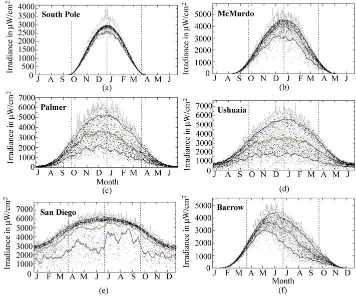
61UV Radiation in Global Climate Change: Measurements, Modeling and Effects on Ecosystems Total ozone at Barrow has been measured by GMD/ESRL with Dobson photometers since 1973. Historical UV intensities for Barrow were calculated in a similar way as UV levels were at South Pole using Dobson measurements from the years 1973 − 1980. Dutton et al. (2004) have reported a statistically significant decrease of effective cloud transmission from 0.64 in 1976 to 0.61 in 2001 based on their analysis of pyranometer data. When estimating past UV Indices, we did not consider this change. First, it is unknown whether the downward trend was already present during the 1960s, and second, changes in cloud transmission were likely smaller in the UV, particularly in spring when attenuation by clouds is reduced by high albedo. To estimate the range of historical UV, we also considered year-to-year changes in surface albedo. The grey area in Fig. 3.8(b) includes changes in total ozone estimated from the years 1973 − 1980, as well as variations due to clouds and albedo estimated from the years 1991 − 2006. UV Indices measured since 1991 are very similar to the historical estimate. For the months February through April, the average increase is 4% − 7% only, and the increase for the 90th percentile is 7% − 13%. Differences for summer months are smaller and may even be negative: recent measurements for August are about 5% below the historical estimate. Differences of this magnitude are within the uncertainty of the data. This shows that there was little change in UV levels during the last 30 years at Barrow, with the exception of several spikes observed during recent low-ozone episodes. 3.4 Climatology of UV-A Irradiance Figure 3.9 shows the climatology of UV-A irradiance (spectral irradiance integrated between 315 nm and 400 nm) for all UVSIMN sites but Summit. All plots show individual measurements, as well as the average, median, and 10th and 90th percentiles, and overall daily maximum. Since long-term changes in cloud cover and albedo are not considered in this study, historical estimates are virtually identical with recent measurements and are therefore not included in Fig. 3.9. Changes in total ozone have practically no influence on UV-A irradiance. Patterns in Fig. 3.9 show mostly seasonal variations in cloudiness, surface albedo, and to a lesser extent, atmospheric aerosol loading. UV-A irradiance at the South Pole is very symmetric about the solstice due to constant high albedo year-round, and little influence by clouds. Daily maximum UV-levels are considerably above the 90th percentile, indicating that enhancement of UV radiation by scattered clouds—which is a well-known effect at mid-latitude sites (Mims and Frederick, 1994)—can also occur at the South Pole. The maximum enhancement is about 30%. Enhancement of the spectral integral 400 nm − 600 nm can be as high as 70%. An extreme example is shown in Fig. 3.10, which displays three spectra measured at 19:00 UT, 19:15 UT, and 19:30 UT on 17 December 2000 at South Pole. During the first spectrum starting at 19:00 UT, the sun was 62
3   Climatology of Ultraviolet Radiation at High Latitudes Derived from Measurements of
     the National Science Foundation’s Ultraviolet Spectral Irradiance Monitoring Network

     Figure 3.9 UV-A irradiance measured at South Pole (Panel (a)), McMurdo (Panel (b)),
     Palmer (Panel (c)), Ushuaia (Panel (d)), San Diego (Panel (e)), and Barrow (Panel (f)).
     Individual measurements, average, median, and 10th and 90th percentiles, as well as
     daily maximum, are shown as in Fig. 3.2(b)

hidden by a stable cloud, leading to a reduction of UV and visible irradiance
of about 10% − 20% compared to the clear-sky model (Fig. 3.10(b), red line).
Measurements were also compared against a second model spectrum where a
wavelength-independent cloud optical depth of 1.83 was used as an additional
model input parameter. The ratio of the measured spectrum with this model
spectrum (Fig. 3.10(b), orange line) is close to one and virtually independent of
wavelength, confirming that the radiation field during the period of the scan
(approximately 13 minutes) was very stable. Measurements of total irradiance
with a pyranometer also indicate constant conditions (Fig. 3.10(c)). During the
second spectrum, starting at 19:15 UT (Fig. 3.10, green lines), total irradiance
increased sharply during the first part of the scan; spectral irradiance increased
up to 60% relative to the clear-sky model. Total irradiance increased by up to 72%.
As reflections from nearby obstacles can be excluded, this pattern can only be
explained by enhancement due to scattered clouds surrounding the (unoccluded)
disk of the sun. Photons passing through a hole in the cloud are scattered multiple
times between the snow-covered surface and the cloud-ceiling. This effect leads to

                                                                                               63
UV Radiation in Global Climate Change: Measurements, Modeling and Effects on Ecosystems
a large enhancement of downwelling radiation and cannot be observed at locations
with small surface albedo. The third spectrum starting at 19:30 UT (Fig. 3.10,
blue lines) agrees well with the clear-sky model. Pyranometer measurements were
close to the value expected for clear-sky.
UV-A irradiance at McMurdo (Fig. 3.9(b)) is generally symmetric about the
solstice. Radiation levels are somewhat smaller in January than December, probably
Figure 3.10 Enhancement of global irradiance by a broken cloud at South Pole.
Panel (a): Three spectra of global irradiance measured on 17-December 2000 at
19:00 UT, 19:15 UT, and 19:30 UT. The clear-sky model spectrum for 19:00 is
also shown. Panel (b): Ratios of measured and modeled spectra. Panel (c): Total
irradiance measured by a pyranometer during the recording of the three spectra and
plotted against the wavelength being sampled by the spectroradiometer as a surrogate
of time
643 Climatology of Ultraviolet Radiation at High Latitudes Derived from Measurements of
the National Science Foundation’s Ultraviolet Spectral Irradiance Monitoring Network
due to smaller albedo in summer when compared with spring. UV-A irradiance at
Palmer (Fig. 3.9(c)) shows a much larger variability than observed at South Pole
and McMurdo due to frequent cloud cover with optical depths typically ranging
between 20 and 50 (Ricchiazzi et al., 1995). The ocean surrounding Palmer freezes
over during the winter. Terrain and glaciers at Palmer are typically covered by snow
up to mid-December. Surface albedo is therefore larger in winter and spring than
in summer. This leads to the small asymmetry in the annual cycle UV-A irradiance
discernable in Fig. 3.9(c). Ushuaia, like Palmer, is affected by persistent cloudiness,
leading to a large difference of the 10th and 90th percentiles (Fig. 3.9(d)). The
Beagle Channel adjacent to Ushuaia does not freeze, but snow typically enhances
the effective surface albedo to approximately 0.2 to 0.3 between June and October,
leading to some enhancement of UV-A during the winter. UV-A irradiance during
spring and summer is almost symmetric about the solstice. The clear-sky limit of
UV-A irradiance at San Diego (Fig. 3.9(e)) is symmetric about the solstice, but the
average and 10th percentile are affected by seasonal patterns in cloudiness. Cloud
attenuation is largest during May and June, whereas most days in August are
cloud-free at solar noon. Enhancement of UV-A irradiance by scattered clouds
beyond the clear-sky limit is remarkably small, and less pronounced than at the
South Pole. This is attributable to low surface albedo ( < 0.05) and the near absence
of broken cumulus clouds, which can enhance UV radiation at other mid-latitude
locations by up to 25% (WMO, 2007). UV-A irradiance at Barrow displays a
strong annual cycle due to seasonal differences in cloudiness (more prevalent in
summer) and surface albedo (0.83 ± 0.08 between November and May; smaller
than 0.1 during summer). The effect of the two factors has been quantitatively
described by Bernhard et al. (2007).
3.5 Comparison of Radiation Levels at Network Sites
There are substantial differences in the UV climatology between the various
UVSIMN sites. A large portion of the differences can be traced to their geographical
locations as lower latitudes experience higher sun elevations and more UV, all
other factors being equal. However, the contention that low levels of UV will
occur in Polar Regions because of the high latitude is shown here to not be true.
Measurements from the seven network sites are presented below. The comparison
is based on the average and maximum UV Index, as well as average and maximum
erythemal daily dose. The results reveal that differences between the sites depend
very much on the selection of the physical quantity used for the comparison.
High levels of UV radiation absorbed during short time-periods, ranging from
minutes to hours, can be most detrimental for some organisms. This includes humans
who may receive a “sunburn” after an exposure time of less than 20 minutes for
UV Indices above 7 (Vanicek et al., 2000). The average noontime and daily
65UV Radiation in Global Climate Change: Measurements, Modeling and Effects on Ecosystems
maximum UV Index are therefore useful for quantifying the risk of getting
sunburned. UV-B radiation is a risk factor for developing basal and squamous
cell carcinoma (Moan and Dahlback, 1992), and the UV Index also provides
guidance in avoiding overexposure with regard to cancer prevention. The “daily
dose” is an appropriate quantity for investigating cumulative UV exposures over
an extended time-period. This is relevant for plants and animals that cannot avoid
the sun. This quantity, however, does not capture the impact of transient high levels
of UV-B that may occur during episodic combinations of clear skies (or partly
cloudy skies and high albedo) and severe ozone depletion. Such incidents may
have biological significance in systems that do not obey reciprocity in terms of
exposure intensity versus duration. This is particularly relevant for microorganisms,
which have only a short life cycle, such as plankton (Moline et al., 1997). The
maximum daily dose may be the best measure for quantifying the effect on these
organisms.
Figure 3.11 shows a comparison of the noontime UV Index from the seven
sites. The data are identical to those indicated by red lines in Figs. 3.4(a), 3.6, and
3.8. Measurements at San Diego exceed those at the other sites due to its lower
latitude, and range between 2.5 during winter and 9.5 during summer.
Figure 3.11 Comparison of average noontime UV Index from all sites
The average noontime UV Index at Palmer, Ushuaia, and Summit, observed close
to the summer solstice, is about 5, or about 55% of the typical summer UV Index
at San Diego. Average UV Indices for South Pole, Barrow and McMurdo extend
up to 2, 3, and 4, respectively. The divergence relative to San Diego is even
larger during autumn and winter when some sites experience extended periods of
darkness.
The differences between sites show completely different patterns when maxima,
rather than average values, are compared. Figure 3.12 shows the maximum daily
UV Index, which was indicated by thin grey lines in Figs. 3.6 and 3.8. At Palmer
Station, the maximum observed UV Index was 14.8. This value is 23% larger than
the highest UV Index of 12.0 measured at San Diego. The maximum UV Index at
663 Climatology of Ultraviolet Radiation at High Latitudes Derived from Measurements of
the National Science Foundation’s Ultraviolet Spectral Irradiance Monitoring Network
Ushuaia was 11.5, which is comparable to summer-time values at San Diego.
Maximum UV Indices at McMurdo, South Pole and Barrow are considerably
smaller than at San Diego; however, the differences are considerably smaller
when compared to average noontime values.
Figure 3.12 Comparison of daily maximum UV Index from all sites, but Summit
The picture changes again when comparing average daily erythemal doses
(Fig. 3.13). The effect of 24 hours of sunlight during Arctic and Antarctic summers
reduces the consequence of latitude differences. Although average summer doses
at San Diego are still highest, average December UV doses at McMurdo, Palmer
Station, South Pole, and Ushuaia, as well as June doses at Summit, amount to
65% − 95% of typical mid-summer San Diego conditions. Note that average daily
doses at McMurdo and South Pole are very similar between mid-January and
March but differ significantly in mid-November when doses at South Pole exceed
those at McMurdo by up to 35%. The reasons are threefold: first, the influence of
the ozone hole on UV-levels is more pronounced at South Pole than at the
Antarctic coast; second, the solar elevation at South Pole is constant for 24 hours;
Figure 3.13 Comparison of average daily erythemal dose from all sites
67UV Radiation in Global Climate Change: Measurements, Modeling and Effects on Ecosystems
and third, albedo at McMurdo is at its annual minimum during January and
February. Average daily erythemal dose at Barrow is the lowest of all network
sites mostly because ozone depletion in the northern hemisphere is much less
severe than over Antarctica.
The importance of UV radiation for high latitudes becomes most obvious when
comparing maximum daily doses. Figure 3.14 shows that the largest daily erythemal
doses ever measured at South Pole and Palmer are 18% and 32%, respectively,
higher than the San Diego record. Maximum doses at McMurdo and Ushuaia are
comparable to San Diego levels. Note that the difference between McMurdo and
South Pole is much smaller when maximum daily doses rather than maximum
noontime UV Indices (Fig. 3.11) are compared. We attribute this to the difference
in the diurnal cycle of the sun at these sites: at McMurdo, radiation levels peak at
local solar noon whereas at the South Pole, there is virtually no change in solar
elevation during a given 24-hour period.
Figure 3.14 Comparison of maximum daily erythemal dose from all sites, but Summit
The effect of 24 hours of sunlight is best shown when comparing the average daily
UV-A dose (Fig. 3.15). Since UV-A spectral irradiance is practically independent
Figure 3.15 Comparison of average daily UV-A dose from all sites
683 Climatology of Ultraviolet Radiation at High Latitudes Derived from Measurements of
the National Science Foundation’s Ultraviolet Spectral Irradiance Monitoring Network
of atmospheric ozone concentrations, there are no ozone-related features in this
figure. UV-A doses at the summer solstice at McMurdo, Summit, and South Pole
exceed San Diego doses by 71% − 88%. In addition to 24 hours of sunlight, this
difference can be explained by high surface albedo, and in the cases of South
Pole and Summit, high altitude.
3.6 Conclusions and Outlook
Measurements of solar UV irradiance performed during the last 18 years at six
high-latitude locations and San Diego have revealed large differences of the sites’
UV climates. The ozone hole has a large effect on the UV Index at the three Antarctic
sites, and to a lesser extent at Ushuaia. UV Indices measured at South Pole during
the ozone hole period are on average 20% − 80% larger than measurements at
comparable solar elevations during summer months. When the ozone hole passed
over Palmer Station late in the year, the UV Index was as high as 14.8 and exceeded
the maximum UV Index of 12.0 observed at San Diego. The maximum UV Index
at Ushuaia was 11.5, which is comparable with summer-time measurements at
San Diego. UV Indices at the two Arctic sites Barrow and Summit are lower than
at southern-hemisphere sites as ozone columns are generally larger in the northern
hemisphere, and ozone depletion is less severe.
A comparison of UV levels at the network sites revealed that differences
between sites depend greatly on the data product used. Average noontime UV
Indices at San Diego during summer are considerably larger than at Antarctic
sites under ozone-hole conditions, but the difference disappears when daily doses
are compared. This contradicts the common notion that UV levels at high
latitudes are small because of small solar elevations.
Reconstructions of historical UV Indices based on long-term ozone records
and climatological cloud and aerosol patterns indicate that contemporary UV
Indices measured during the ozone hole period at Antarctic sites are on average
30% − 85% larger than estimates for the past. These reconstructions were based
on the assumption that cloud, albedo, and aerosol conditions have not changed
over the last 40 years. Analysis of pyranometer data from South Pole and Barrow
indicated that this assumption is justified. Similar long-term observations are not
available from other UVSIMN locations, and estimates of historical UV irradiance
at those sites are therefore more uncertain. Clearly, the reconstruction of UV levels
from proxy data has a larger uncertainty than actual measurements. Operation of
the UVSIMN is expected to continue, providing the opportunity to assess future
developments of high-latitude UV climate more accurately than in the past. These
measurements will help document changes in UV levels due to the expected
recovery of the ozone layer (WMO, 2007) and the impact of climate change, which
will likely modify stratospheric temperatures; ozone (column and profile); surface
69UV Radiation in Global Climate Change: Measurements, Modeling and Effects on Ecosystems albedo (e.g., due to changes in the timing of snow melt (Stone et al., 2002)); clouds (frequency and optical properties), aerosols (e.g., changes in Arctic haze (Bodhaine and Dutton, 1993)), and atmospheric circulation patterns (Knudsen and Anderson, 2001). Acknowledgements Operation of the UVSIMN and this study were supported by the National Science Foundation’s Office of Polar Programs via a subcontract to Biospherical Instru- ments Inc. from Raytheon Polar Services Company (RPSC). Extended thanks go to Vi Quang of BSI for assisting in data processing. Dobson measurements for South Pole and Barrow were retrieved from http://www.esrl.noaa.gov/gmd/ozwv/dobson/. TOMS Nimbus-7 total ozone data were accessed via the website http://toms.gsfc.nasa.gov/n7toms/n7_ovplist_a.html. We thank Ellsworth Dutton from NOAA for discussions regarding cloud effects at the South Pole. References Bernhard G, Booth CR, and Ehramjian JC (2004) Version 2 Data of the National Science Foundation’s Ultraviolet Radiation Monitoring Network: South Pole. J. Geophys. Res. 109:D21207, doi:10.1029/2004JD004937 Bernhard G, Booth CR, and Ehramjian JC (2005) UV Climatology at Palmer Station, Antarctica. In: Bernhard G, Slusser JR, Herman JR, Gao W (eds) Ultraviolet Ground- and Space-based Measurements, Models, and Effects V. Proceedings of SPIE International Society of Optical Engineering 5886, pp 588607-1 − 588607-12 Bernhard G, Booth CR, Ehramjian JC, and Quang VV (2006a) NSF Polar Programs UV Spectroradiometer Network 2004 − 2005 Operations Report, Volume 14.0, 257 pp, Biospherical Instruments Inc., San Diego, CA, http://www.biospherical.com/NSF Bernhard G, Booth CR, Ehramjian JC, and Nichol SE (2006b) UV climatology at McMurdo Station, Antarctica, Version 2 Data of the National Science Foundation’s Ultraviolet Radiation Monitoring Network. J. Geophys. Res. 111:D11201, doi:10.1029/2005JD005857 Bernhard G, Booth CR, Ehramjian JC, Stone R, and Dutton EG (2007) Ultraviolet and visible radiation at Barrow, Alaska: Climatology and influencing factors on the basis of Version 2 National Science Foundation network data. J. Geophys. Res. 112:D09101, doi:10.1029/ 2006JD007865 Bernhard G, Booth CR, and Ehramjian JC (2008) Comparison of UV irradiance measurements at Summit, Greenland; Barrow, Alaska; and South Pole. Antarctica. Atmos. Chem. Phys. 8: 4799 − 4810, http://www.atmos-chem-phys.net/8/4799/ Bodhaine BA and Dutton EG (1993) A long-term decrease in Artic haze at Barrow, Alaska. Geophys. Res. Lett. 20: 947 − 950 70
3   Climatology of Ultraviolet Radiation at High Latitudes Derived from Measurements of
     the National Science Foundation’s Ultraviolet Spectral Irradiance Monitoring Network

Booth CR, Lucas TB, Morrow JH, Weiler CS, and Penhale PA (1994) The United States National
    Science Foundation’s polar network for monitoring ultraviolet radiation. Weiler CS,
    Penhale PA (eds). Antarc. Res. Ser. 62: 17 − 37
Chubachi S (1984) Preliminary results of ozone observations at Syowa Station from February
    1982 to January 1983. Mem. Natl. Inst. Polar Res. Jap., Spec. Issue 34: 13 − 19
Climate Monitoring and Diagnostics Laboratory (CMDL) (2004) Summary Report 27,
    2002 − 2003. Schnell RC, Buggle A-M, Rosson RM (eds) U.S. Dept. of Commerce,
    Boulder, CO
Dutton EG, Farhadi A, Stone RS, Long CN, and Nelson DW (2004) Long-term variations in
    the occurrence and effective solar transmission of clouds as determined from surface-based
    total irradiance observations. J. Geophys. Res. 109:D03204, doi:10.1029/2003JD003568
Farman JC, Gardiner BG, and Shanklin JD (1985) Large losses of total ozone in Antarctica
    reveal seasonal ClOx/NOx interaction. Nature 315: 207 − 210
Fioletov VE, McArthur LJB, Kerr JB, and Wardle DI (2001) Long-term variations of
    UV-B irradiance over Canada estimated from Brewer observations and derived from
    ozone and pyranometer measurements. J. Geophys. Res. 106(D19): 23009 − 23028,
    10.1029/2001JD000367
Grenfell TC, Warren SG, and Mullen PC (1994) Reflection of solar radiation by the Antarctic
    snow surface at ultraviolet, visible, and near infrared wavelengths. J. Geophys. Res.
    99(D9): 18669 − 18684
Gröbner J, Blumthaler M, Kazadzis S, Bais A, Webb A, Schreder J, Seckmeyer G, and Rembges
    D (2006) Quality assurance of spectral solar UV measurements: results from 25 UV monitoring
    sites in Europe, 2002 to 2004. Metrologia 43: S66 − S71, doi:10.1088/0026-1394/43/2/S14
Holton JR, Haynes PH, McIntyre ME, Douglass AR, Rood RB, and Pfister L (1995)
    Stratosphere-troposphere exchange. Rev. Geophys. 33(4): 403 − 440
Kaye JA, Hicks BB, Weatherhead EC, Long CS, and Slusser JR (1999) U.S. Interagency UV
    Monitoring Program established and operating. EOS 80(10): 113 − 116
Knudsen BM and Andersen SB (2001) Longitudinal variation in springtime ozone trends
    Nature 413: 699 − 700
Mayer B and Kylling A (2005) Technical note: the libRadtran software package for radiative
    transfer calculations — description and examples of use. Atmos. Chem. Phys. 5: 1855 − 1877,
    http://www.atmos-chem-phys.org/acp/5/1855/
McKenzie R, Connor B, and Bodeker G (1999) Increased summertime UV radiation in New
    Zealand in response to ozone loss. Science 285(5434): 1709 − 1711, DOI:10.1126/science.
    285.5434.1709
McKinlay AF and Diffey BL (eds) (1987) A reference action spectrum for ultraviolet induced
    erythema in human skin. In: Commission International de l’Éclairage (CIE). Research
    Note 6(1): 17 − 22
McPeters RD and Labow GJ (1996) An assessment of the accuracy of 14.5 years of Nimbus 7
    TOMS Version 7 ozone data by comparison with the Dobson network. Geophys. Res. Lett.
    23(25): 3695 − 3698
Mims FM and Frederick JE (1994) Cumulus clouds and UVB. Nature 371: 291
Moan J and Dahlback A (1992) The relationship between skin cancers, solar radiation, and
    ozone depletion. British Journal of Cancer 65: 916 − 921

                                                                                            71
UV Radiation in Global Climate Change: Measurements, Modeling and Effects on Ecosystems
Moline MA, Prézelin BB, Schofield O, and Smith RC (1997) Temporal dynamics of coastal
Antarctic phytoplankton: environmental driving forces and impact of a 1991/1992 summer
diatom bloom on the nutrient regimes. In: Battaglia B, Valencia J, Walton DWH (eds)
Antarctic Communities. Cambridge Press, London, 67 − 72
Nichol SE, Pfister G, Bodeker GE, McKenzie RL, Wood SW, and Bernhard G (2003) Moderation
of cloud reduction of UV in the Antarctic due to high surface albedo. J. Appl. Meteorol.
42(8): 1174 − 1183
Rex M, Salawitch RJ, von der Gathen P, Harris NRP, Chipperfield MP, and Naujokat
B (2004) Arctic ozone loss and climate change. Geophys. Res. Lett. 31:L04116,
doi:10.1029/2003GL018844
Ricchiazzi P, Gautier C, and Lubin D (1995) Cloud scattering optical depth and local surface
albedo in the Antarctic: simultaneous retrieval using ground-based radiometry. J. Geophys.
Res. 100(D10): 21091 − 21104
Shaw GE (1982) Atmospheric turbidity in the Polar regions. J. Appl. Meteorol. 21: 1080 − 1088
Seckmeyer G, Erb R, and Albold A (1996) Transmittance of a cloud is wavelength-dependent
in the UV-range. Geophys. Res. Lett. 23(20): 2753 − 2756
Stone RS, Dutton EG, Harris JM, and Longenecker D (2002) Earlier spring snowmelt in
northern Alaska as an indicator of climate change. J. Geophys. Res. 107(D10): 4089,
doi:10.1029/2000JD000286
Vanicek K, Frei T, Litynska Z, and Schmalwieser A (2000) UV-Index for the public, COST-713
Action. Office for Official Publications of the European Communities, Luxembourg. ISBN
92-828-8142-3, 27
Weatherhead EC, Reinsel CG, Tiao GC, Meng X-L, Choi D, Cheang W-K, Keller T, DeLuisi JJ,
Wuebbles DJ, Kerr JB, Miller AJ, Oltmans SJ, and Frederick JE (1998) Factors affecting
the detection of trends: statistical considerations and applications to environmental data.
J. Geophys. Res. 103(D14): 17149 − 17161
World Health Organization (WHO) (2002) Global solar UV Index: a practical guide. ISBN
9241590076, Geneva, Switzerland. http://www.unep.org/PDF/Solar_Index_Guide.pdf. 28 pp
World Meteorology Organization (WMO) (2007) Scientific assessment of ozone depletion: 2006,
Global ozone research and monitoring project, Geneva, Switzerland, Report No. 50, 572 pp
72You can also read