A Theory of High Dimensional Regression with Arbitrary Correlations between Input Features and Target Functions: Sample Complexity, Multiple ...
←
→
Page content transcription
If your browser does not render page correctly, please read the page content below
A Theory of High Dimensional Regression with Arbitrary Correlations
  between Input Features and Target Functions: Sample Complexity, Multiple
            Descent Curves and a Hierarchy of Phase Transitions

                                             Gabriel C. Mel 1 Surya Ganguli 2

                         Abstract                               understanding the ability of not only deep networks, but also
                                                                many other machine learning (ML) methods, to successfully
     The performance of neural networks depends on              generalize to test examples drawn from the same distribution
     precise relationships between four distinct ingre-         as the training data. Such theory would ideally guide the
     dients: the architecture, the loss function, the sta-      choice of various ML hyperparameters to achieve minimal
     tistical structure of inputs, and the ground truth         test error.
     target function. Much theoretical work has fo-
     cused on understanding the role of the first two           However, any such theory that is powerful enough to guide
     ingredients under highly simplified models of ran-         hyperparameter choices in real world settings necessarily
     dom uncorrelated data and target functions. In             involves assumptions about the nature of the ground truth
     contrast, performance likely relies on a conspir-          mapping to be learned, the statistical structure of the inputs
     acy between the statistical structure of the input         one has access to, the amount of data available, and the ma-
     distribution and the structure of the function to be       chine learning method itself. Many theoretical works study-
     learned. To understand this better we revisit ridge        ing the generalization properties of ML methods have made
     regression in high dimensions, which corresponds           highly simplified assumptions about the statistical structure
     to an exceedingly simple architecture and loss             of inputs and the ground truth mapping to be learned.
     function, but we analyze its performance under             Much work in computer science for example seeks to find
     arbitrary correlations between input features and          worst case bounds on generalization error over the choice
     the target function. We find a rich mathematical           of the worst data set and the worst ground truth function
     structure that includes: (1) a dramatic reduction          (Vapnik, 1998). Such bounds are often quite pessimistic
     in sample complexity when the target function              as the types of data and ground truth functions that occur
     aligns with data anisotropy; (2) the existence of          in natural problems are far from worst case. These worst
     multiple descent curves; (3) a sequence of phase           case bounds are then often vacuous (Zhang et al., 2017) and
     transitions in the performance, loss landscape, and        cannot guide choices made in practice, spurring the recent
     optimal regularization as a function of the amount         search for nonvacuous data-dependent bounds (Dziugaite &
     of data that explains the first two effects.               Roy, 2017).
                                                                Also, much work in statistical physics has focused instead
                                                                on computing exact formulas for the test error of various
1. Introduction and Motivation
                                                                ML algorithms (Engel & den Broeck, 2001; Advani et al.,
The field of machine learning, especially in the form of deep   2013; Advani & Ganguli, 2016a;b) including compressed
learning, has undergone major revolutions in the last several   sensing (Rangan et al., 2009; Donoho et al., 2009; Ganguli
years, leading to significant advances in multiple domains      & Sompolinsky, 2010b;a), single layer (Seung et al., 1992)
(LeCun et al., 2015). Many works have attempted to gain a       and multi-layer (Monasson & Zecchina, 1995; Lampinen
theoretical understanding of the key reasons underlying the     & Ganguli, 2018) neural networks, but under highly sim-
empirical success of deep neural networks (see e.g. (Bahri      plified random uncorrelated assumptions about the inputs.
et al., 2020) for a review). A major open puzzle concerns       Moreover, the ground truth target function was often chosen
  1
                                                                randomly in a manner that was uncorrelated with the choice
    Neurosciences PhD Program, School of Medicine, Stanford     of the random inputs. In most situations where the ground
University, CA, US 2 Department of Applied Physics, Stanford,
CA, US. Correspondence to: G.C. Mel .       truth function possessed no underlying simple structure,
                                                                these statistical physics works based on random uncorre-
Proceedings of the 38 th International Conference on Machine    lated functions and inputs generally concluded that the ratio
Learning, PMLR 139, 2021. Copyright 2021 by the author(s).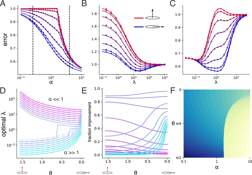
An Analytic Theory of High Dimensional Regression with Correlated Inputs and Aligned Targets

of the number of data points must be proportional to the          generalizing the phenomenon of double descent (Belkin
number of unknown parameters in order to achieve good             et al., 2019; Mei & Montanari, 2020; d’Ascoli et al., 2020);
generalization. In practice, this ratio is much less than 1.      (6) we analytically compute the spectrum of the Hessian of
                                                                  the loss landscape and show that this spectrum undergoes
A key, and in our view foundational ingredient underlying
                                                                  a sequence of phase transitions as successively finer scales
the theory of generalization in ML is an adequate model
                                                                  become visible with more data; (7) we connect these spec-
of the statistical structure of the inputs, the nature of the
                                                                  tral phase transitions to the phenomenon of multiple descent
ground truth function to be learned, and most importantly,
                                                                  and to phase transitions in the optimal regularization.
an adequate understanding of how the alignment between
these two can potentially dramatically impact the success of      Finally, we note that the phenomenon of double descent
generalization. For example, natural images and sounds all        in a generalization curve refers to non-monotonic behavior
have rich statistical structure, and the functions we wish to     in this curve, corresponding to a single intermediate peak,
learn in these domains (e.g. image and speech recognition)        as a function of the ratio of the number data points to pa-
are not just random functions, but rather are functions that      rameters. This can occur either when the amount of data is
are intimately tied to the statistical structure of the inputs.   held fixed and the number of parameters increases (Belkin
Several works have begun to explore the effect of structured      et al., 2019; Mei & Montanari, 2020; d’Ascoli et al., 2020;
data on learning performance in the context of compressed         Chen et al., 2021), or when the number of parameters is
sensing in a dynamical system (Ganguli & Sompolinsky,             held fixed but the amount of data increases (Seung et al.,
2010a), the Hidden Manifold Model (Goldt et al., 2020;            1992; Engel & den Broeck, 2001). Here we exhibit multiple
Gerace et al., 2020), linear and kernel regression (Chen          descent curves with arbitrary numbers of peaks in the latter
et al., 2021; Canatar et al., 2021), and two-layer neural         setting. We explain their existence in terms of a hierarchy of
networks (Ghorbani et al., 2020). As pointed out by these         phase transitions in the empirical covariance matrix of multi-
authors, it is likely the case that a fundamental and still       scale correlated data. And furthermore, we show that such
poorly understood conspiracy between the structure of the         non-monotonic behavior is a consequence of suboptimal
inputs we receive and the aligned nature of the functions we      regularization. Indeed we show how to recover monotoni-
seek to compute on them plays a key role in the success of        cally decreasing generalization error curves with increasing
various ML methods in achieving good generalization.              amounts of data by using an optimal regularization that
                                                                  depends on the ratio of data points to parameters.
Therefore, with these high level motivations in mind, we
sought to develop an asymptotically exact analytic theory of
generalization for ridge regression in the high dimensional       2. Overall Framework
statistical limit where the number of samples N and number
                                                                  Generative Model. We study a generative model of data
of features P are both large but their ratio is O(1). Ridge
                                                                  consisting of N independent identically distributed (iid)
regression constitutes a widely exploited method especially
                                                                  random Gaussian input vectors xµ ∈ RP for µ = 1, . . . , N ,
for high dimensional data; indeed it was shown to be optimal
                                                                  each drawn from a zero mean Gaussian with covariance
for small amounts of isotropic but non-Gaussian data (Ad-
                                                                  matrix Σ (i.e. xµ ∼ N (0, Σ)), N   corresponding iid scalar
vani & Ganguli, 2016a;b). Moreover the high dimensional
                                                                  noise realizations µ ∼ N 0, σ 2 , and N outputs y µ given
statistical limit is increasingly relevant for many fields in
                                                                  by
which we can simultaneously measure many variables over
                                                                                       y µ = x µ · w + µ ,
many observations. The novel ingredient we add is that we
assume the inputs have an arbitrary covariance structure,         where w ∈ RP is an unknown ground truth regression
and the ground truth function has an arbitrary alignment          vector. The outputs y µ decompose into a signal component
with this covariance structure. We focus in particular on         xµ · w and noise component µ and signal to noise ratio
examples involving highly heterogeneous multi-scale data.         (SNR) given by the relative power
Our key contributions are: (1) We derive exact analytic
formulas for test error in high dimensions; (2) we show                                   Var[x · w]   wT Σw
                                                                                SN R :=              =       ,              (1)
that for a random target function, isotropic data yields the                                Var[]      σ2
lowest error; (3) we demonstrate that for anisotropic data,
alignment of the target function with this anisotropy yields      plays a critical role in estimation performance. For conve-
lowest test error; (4) we derive an analytic understanding        nience below we also define the fractional signal power
                                                                                T
of the optimal regularization parameter as a function of the      fs := wTwΣw+σ   Σw
                                                                                      2 and fractional noise power fn     :=
structure of the data and target function; (5) for multi-scale        σ2                                        fs
                                                                  wT Σw+σ 2
                                                                            .   Note fs + fn = 1 and SN R =     fn .
data we find a sequence of phase transitions in the test error
and the optimal regularization parameter that result in multi-    High Dimensional Statistics Limit. We will be working
ple descent curves with arbitrary numbers of peaks, thereby       in the nontrivial high dimensional statistics limit where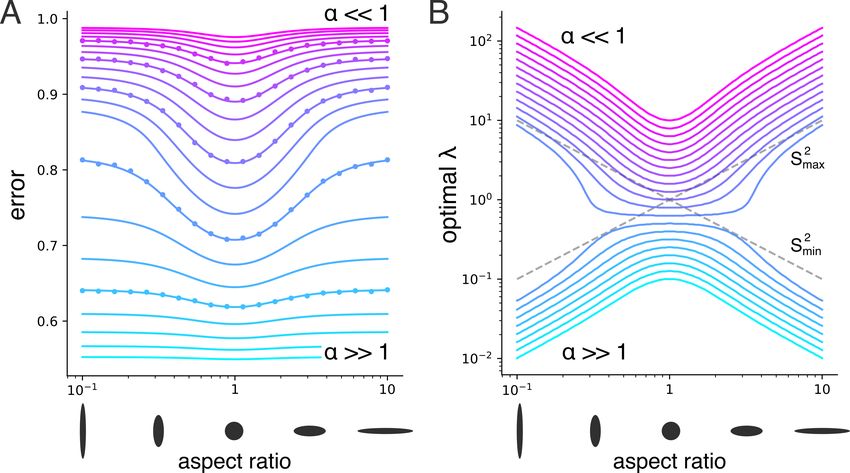
An Analytic Theory of High Dimensional Regression with Correlated Inputs and Aligned Targets
N, P → ∞ but the measurement density α = N/P re- 3. Results
mains O(1). We assume that Σ has P eigenvalues that
are each O(1) so that both σx2 := P1 E xT x = P1 Tr Σ and 3.1. Exact High Dimensional Error Formula.
the individual components of x remain O(1) as P → ∞. Our first result is a formula for F for arbitrary α, σ 2 , Σ, w
T
√ that w w is O(1) (i.e. each
Furthermore we assume com- and λ,that is asymptotically exact in the high dimensional
ponent of w is O(1/ P ) and the noise variance σ 2 is O(1) statistical limit. To understand this formula, it is useful to
so that the SN R remains O(1). first compare to the scalar case where P = 1 and N is large
but finite. Σ then has a single eigenvalue S 2 and F in this
Estimation Procedure. We construct an estimate ŵ of w scalar case is given by (see SM for details)
from the data {xµ , y µ }N
µ=1 using ridge regression: 2 2
S2
λ 1
Fscalar ≈ fn +fs +f n . (5)
N S2 + λ N S2 + λ
1 X µ 2
ŵ = arg min (y − xµ · w) + λ||w||2 . (2) The first term comes from unavoidable noise in the test ex-
w N µ=1
ample. The second term originates from the discrepancy
between ŵ and w. Since increasing λ shrinks ŵ away from
The solution to this optimization problem is given by w leading to underfitting, this second term increases with
−1 increasing regularization. The third term originates primar-
ŵ = XT X + λN IP XT y, (3) ily from the noise in the training data. Since increasing λ
reduces the sensitivity of ŵ to this training noise, this third
where X is an N ×P matrix whose µth row is xµT , y ∈ RN term decreases with increasing regularization. Balancing
with components y µ and IP is the P × P identity matrix. underfitting versus noise reduction sets an optimal λ. In-
creasing (decreasing) the SN R increases (decreases) the
Performance Evaluation. We will be interested in the weight of the second term relative to the third, tilting the
fraction of unexplained variance F on a new test example balance in favor of a decreased (increased) optimal λ.
(x, , y), averaged over realizations of the inputs xµ and Our main result is that in the high dimensional anisotropic
noise µ that determine the training set: setting we obtain a similar formula
!2 !2
P
h i
2 2
Exµ ,µ ,x, (y − x · ŵ) 1 X λ̃ 1 1 Si
F := . (4) F = fn + fs v̂i2 + f n ,
Ex, [y 2 ] ρf i=1
Si2 + λ̃ α P Si2 + λ̃
(6)
In the high dimensional statistics limit, the error F will but with several fundamental modifications compared to
concentrate about its mean value, and will depend upon the the low dimensional setting, as can be seen by comparing
measurement density α, the noise level σ 2 , the input covari- (5) and (6). First the original regularization parameter λ
ance Σ, the ground truth vector w and the regularization λ. is replaced with an effective regularization parameter λ̃.
In particular we will be interested in families of problems Second, the single scalar mode is replaced with an average
of the same SN R but with varying degrees of alignment over the P eigenmodes of Σ. Third, the scalar measurement
between the ground truth w with eigenspaces of Σ. density N is converted to the high dimensional measurement
density α. Fourth, there is an excess multiplicative factor on
the last two terms of the error that increases as the fractional
Models of Multi-Scale Covariance Matrices. The align-
participation ratio ρf decreases. We now define and discuss
ment of w with different eigenspaces of Σ (at fixed SN R)
each of these important elements in turn.
becomes of particular interest when Σ contains a hierar-
chy of multiple scales. In particular consider a D scale
model in which Σ has D distinct eigenvalues Sd2 for d = The Effective Regularization λ̃. As we show through ex-
1, tensive calculations in SM (which we sketch in section 3.7)
P.D. . , D where each eigenvalue has multiplicity Pd where a key quantity that governs the performance of ridge regres-
d=1 Pd = P . A special case is the isotropic single scale
model where Σ = S12 IP . Another important special case is sion in high dimensions is the inverse Hessian of the cost
the anisotropic two scale model with two distinct eigenval- function in (2). This inverse Hessian appears in the estimate
−1
ues S12 and S22 with multiplicities P1 and P2 , corresponding of ŵ in (3) and is given by B := N1 XT X + λIP . A
−1
closely related matrix is B̃ := N1 XXT + λIN
to long and short data directions. Throughout we will quan- . Indeed
tify the input anisotropy via the aspect ratio γ := SS12 (with the two matrices have identical spectra except for the num-
γ = 1 reducing to isotropy). For simplicity, we will balance ber of eigenvalues equal to λ, corresponding to the zero
the number of long and short directions (i.e. P1 = P2 ). eigenvalues of XT X and XXT . The effective regulariza-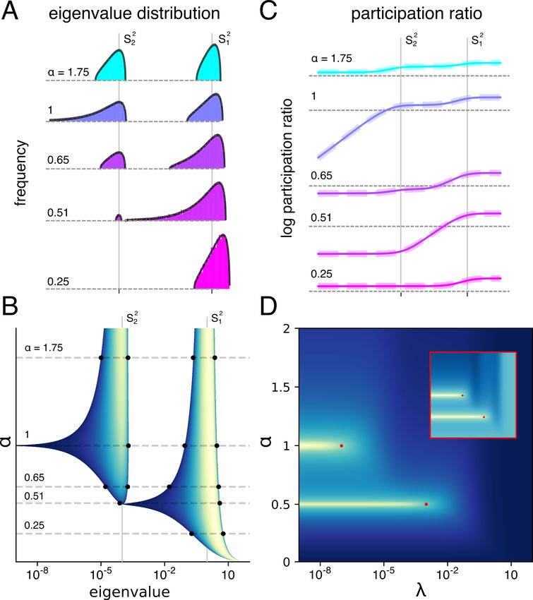
An Analytic Theory of High Dimensional Regression with Correlated Inputs and Aligned Targets
tion λ̃ can be expressed in terms of the spectrum of B̃ via expand this matrix inverse as a power series:
X 1 n
1 1 T
−1 n T
λ̃ := 1/ Tr B̃ . (7) B = X X + λN IP = −z z X X ,
N N n
N
(10)
In the high dimensional limit, λ̃ converges to the solution of
where z = − λ1 . This series is a generating function for
n
P the matrix sequence An = N1 XT X . We show that
1 1 X λ̃Sj2
λ = λ̃ − , (8) computing the average of An over the training inputs X
α P j=1 λ̃ + Sj2 reduces to a combinatorial problem of counting weighted
as we prove in SM . We will explore the properties of the paths (weighted by the eigenvalues of Σ) of length 2n in
effective regularization and its dependence on λ, α, and the a bipartite graph with two groups of nodes corresponding
spectrum of Σ in more detail in Sec. 3.3. to the N samples and P features respectively. In the limit
N, P → ∞ for fixed α = N/P we further show that only
paths whose (paired) edges form a tree contribute to An .
The Target-Input Alignment v̂i2 . In the third term, all
Thus we show the matrix inverse in (10) averaged over the
P modes are equally averaged via the factor P1 while in
training data X is a generating function for weighted trees
the second term, each mode is averaged with a different
embedded in a bipartite graph. We further exploit the recur-
weight v̂i2 which captures the alignment between the target
sive structure of such trees to produce a recurrence relation
function w and the input distribution. To define this weight,
satisfied by the An averaged over X. This recurrence re-
let the eigendecomposition of the true data covariance be
2 T lation yields recursive equations for both the generating
given by Σ = USP U . The total signal power can be
function in (10) and the effective regularization λ̃ in (8).
written w Σw = i vi2 , where v = SUT w, so that the
T
From these recursive equations we also finally obtain the
components vi2 can be interpreted as the signal power in
formula for the error F in (6) averaged over all the training
the ith mode of the data. v̂ in (6) is defined to be the unit
and test data (see SM ).
vector in the same direction as v, so the components v̂i2
quantify the fractional signal power in the ith mode. Both
vT v = wT Σw and v̂T v̂ = 1 are O(1), so vi2 and v̂i2 are 3.3. Properties of Effective Regularization λ̃ and
O(1/P ), and so the second term in (6) has a well defined Fractional Participation Ratio ρf
high dimensional limit. Thus the second term in (6) can be We show that the effective regularization λ̃ is an increasing,
thought of as a weighted average over each mode i, where concave function of λ satisfying (see SM )
the weight v̂i2 is the fractional signal power in that mode.
σx2
λ ≤ λ̃ ≤ λ + . (11)
The Fractional Participation Ratio ρf . We define the α
participation ratio ρ of the spectrum of B̃ as
Furthermore, for large λ, λ̃ tends to the upper bound in (11)
2 with error O(1/λ). Thus, when λ is large enough, λ̃ can
Tr B̃ be thought of as λ plus a constant correction σx2 /α which
ρ := . (9)
Tr B̃2 vanishes in the oversampled low dimensional regime of
large α.
ρ measures the number of active eigenvalues in B̃ in a scale-
The important qualitative features of λ̃ can be illustrated in
invariant manner, and always lies between 1 (when B̃ has a
the isotropic case, where
single nonzero eigenvalue) and N (when B̃ has N identical
eigenvalues) (see SM ). The fractional participation ratio q 2
is then ρf := ρ/N which satisfies N1 ≤ ρf ≤ 1. For a λ + S 2 α1 − 1 + λ + S 2 α1 + 1 − 4 α1 S 4
λ̃ = .
typical spectrum, the numerator in (9) is O(N 2 ) and the 2
denominator is O(N ), so ρ = O(N ) and ρf = O(1). We (12)
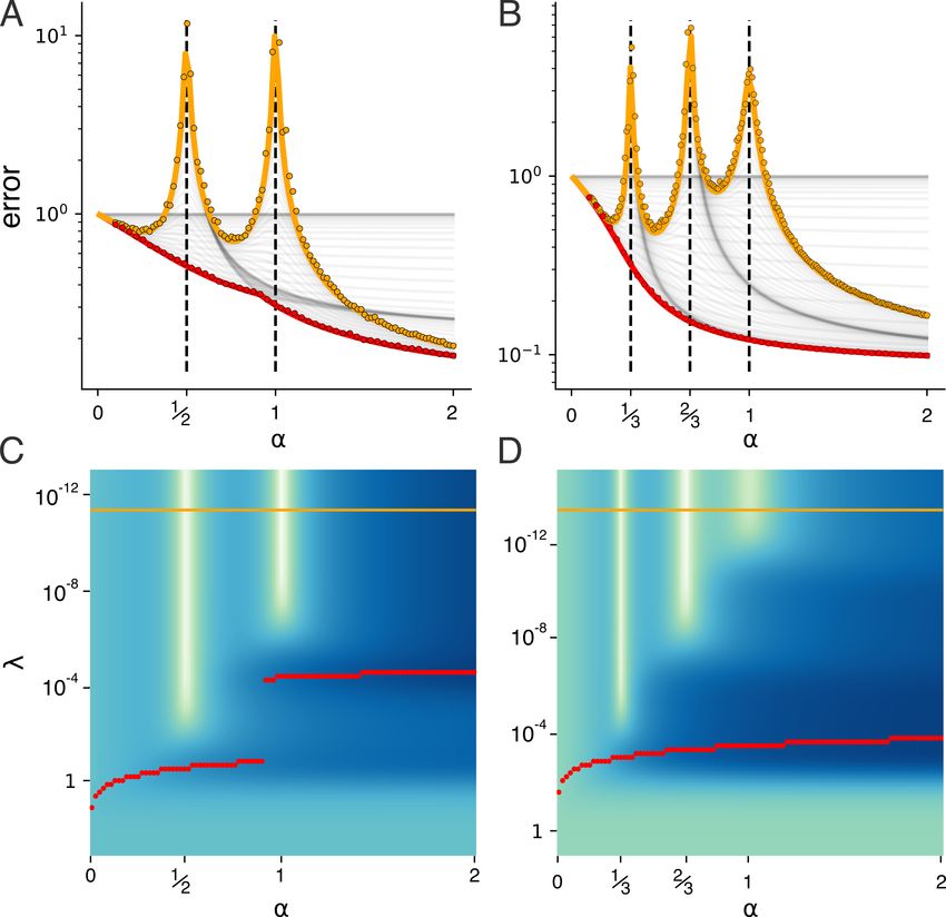
For α > 1, the graph of λ̃(λ) rises from the origin and
also prove a relation between ρf and λ̃ (see SM ): ddλλ̃ = ρ1f .
gradually approaches the line λ̃ = λ + S 2 /α, coinciding
Thus a high sensitivity of the effective regularization λ̃ to with the upper bound in (11) (Figure 1A; cyan curves). As
changes in the actual regularization λ coincide with reduced α is decreased the slope at the origin becomes steeper until,
participation ratio ρf and higher error F in (6). at the critical value α = 1, the slope ddλλ̃ at λ = 0 is infinite.
After this point for α < 1, λ̃ has nonzero y-intercept (Figure
3.2. Proof Sketch of High Dimensional Error Formula. 1A, magenta curves; B shows zoomed in view with critical
We first insert (3) into (4) and average over all variables α = 1 curve in black). Figure 1C and D show λ̃ and 1/ρf
except X, which appear inside a matrix inverse. We then as a joint function of λ, α. Recalling that ρ1f = ddλλ̃ , the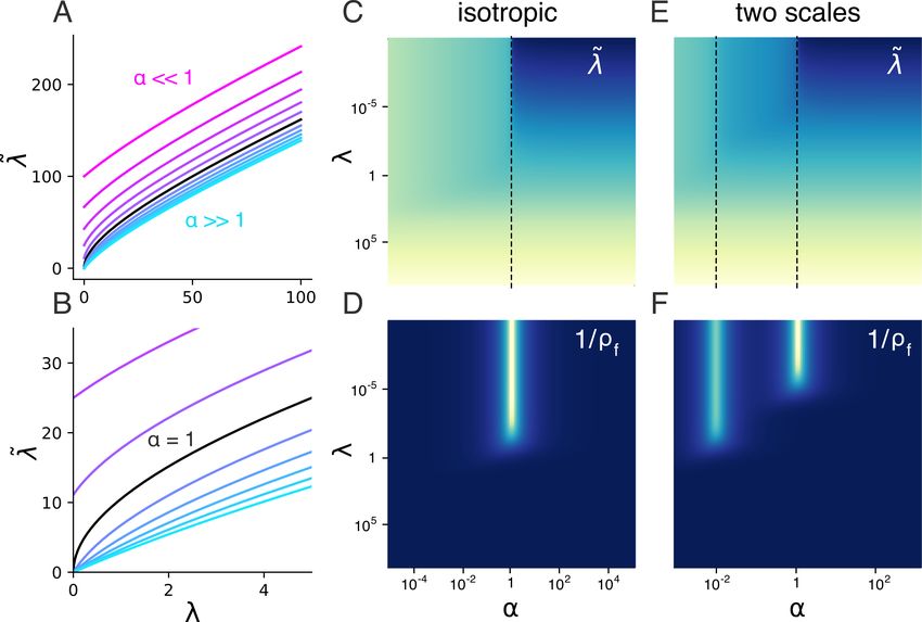
An Analytic Theory of High Dimensional Regression with Correlated Inputs and Aligned Targets
bright bar in D representing small ρf corresponds exactly to value of the fractional SNR per mode v̂i2 = 1/P in (6).
λ̃’s infinite derivative at α = 1 (Figure 1B; C, dashed line).
Thus large sensitivity in λ̃ to changes in λ corresponds to a
small fractional participation ratio ρf , which in turn leads
to increased error in (6). For a covariance with multiple
distinct scales, λ̃ behaves analogously, and can attain near
infinite slope at more than one critical value of α (two scale
model shown in Figure 1E,F). We observe in 3.6 that this
can lead to multiple descent curves, and in 3.7 we show how
these effects can be understood in terms of the spectrum of
the inverse Hessian B.
Figure 2. Learning a random function is easiest with isotropic data.
A: Error as a function of data anisotropy in a model with 2 dis-
tinct variances (diagrams below x-axis show relative length scales
of the data distribution). Different traces correspond to different
measurement densities α. λ is optimized (either empirically or
using the error formula (6)) for each α and aspect ratio. Across
different α’s, error is minimized on isotropic input data distribu-
tions. Dots showing average error from actual ridge regression at
5 α’s (P1 = P2 = 50, P = 100 and N = 25, 50, 100, 200, 400)
closely match theoretical curves. B: Optimal λ as a function of
the data distribution’s aspect ratio. Traces and colors correspond
to A. Dashed lines show the value of the large and small variance.
For highly anisotropic data, the optimal λ jumps suddenly from
2 2
∝ Smin to ∝ Smax as α increases (note the sudden jump in cyan
Figure 1. λ̃ is the effective regularization parameter satisfying (8). to magenta curves (decreasing α) at the extremal aspect ratios).
A: λ̃ vs λ for different values of α. In all cases λ̃ tends to λ plus a
constant positive correction factor (see (11)). In the undersampled
regime α
1, the intercept is nonzero (magenta traces), while For a two-scale model the main parameter of interest is
in the oversampled regime the intercept is zero (cyan traces). B: the aspect ratio γ = S1 /S2 . Figure 2A shows the error
Zooming in on the traces in A shows that at α = 1 the slope F in (6), optimized over λ, as a function of γ (with total
dλ̃
dλ
becomes infinite, separating the cases with zero and nonzero SN R held constant as γ varies), for different values of the
intercept. Right heatmaps: upper row, λ̃ as a function of α, λ; measurement density α. The dots correspond to results
bottom row, 1/ρf . Brighter colors indicate higher values. For from ridge regression, which shows excellent agreement
the isotropic case with S 2 = 1 (C,D), and similarly for slightly with the theoretical curves. For all α, F is minimized when
anisotropic cases, λ̃, ρf behave as the traces shown in A,B. For γ = 1, demonstrating that for a generic unaligned target
two widely separated scales (S1 , S2 = 1, 10−2 , and PP1 , PP2 = function, error at constant SNR is minimized when the data
1
, 100 ; these values were chosen to illustrate the behavior of λ̃.
101 101 is isotropic.
For all other figures, P1 = P2 unless stated otherwise.) (E,F), λ̃
has a near infinite derivative at two critical values of α. We show Figure 2B shows the optimal λ as a function of aspect ra-
below that this has consequences for the error when fitting with tio. As expected, optimal regularization decreases with α,
highly anisotropic data. reflecting the fact that as the number of training examples
increases, the need to regularize decreases. More interest-
ingly, crossing the boundary between undersampled and
3.4. Input Anisotropy Increases Error for Generic oversampled around α = O(1), the optimal regularization
2 2
Target Functions undergoes a sudden jump from ≈ Smax to ≈ Smin (diag-
onal dashed lines). Consistent with this, we show in SM
We first address how anisotropy in Σ alone affects perfor-
that when the aspect ratio is very large or small, the optimal
mance when there is no special alignment between w and
regularization λ∗ takes the following values in the under-
Σ. To this end we draw w from a zero mean Gaussian with
and over-sampled limits:
covariance C = σ 2 SNPR0 Σ−1 . This choice essentially fixes (
T 1 1 2
the expected SN R = w σΣw to the constant value SN R0 ∗ R Smin α
1
2
λ → α1 SN 1 1 2
(13)
and spreads it evenly across the modes, with the expected α 2 + SN R S max α
1.An Analytic Theory of High Dimensional Regression with Correlated Inputs and Aligned Targets
This can be roughly understood as follows: in the under-
sampled regime, where strong regularization is required to
1 σ 2 P1 Tr [Σ−1 ] α
1
control λ̃ should be increased until the third term in
noise, 2 λ∗ → α wT Σ−1 w (14)
Si2 2 1 σ 2 (1 + SN R) 1
Tr [Σ2 ] 2
σx
(6), Si2 +λ̃
, stops improving, around λ̃ ≈ Smax .
On the α
P
wT Σ2 w
− α α
1
other hand, in the oversampled regime, where the weights
can be estimated reliably and the biggest source of error These approximate formulas are plotted in Figure 3D
is underfitting from the regularization itself, λ̃ should be (dashed lines), and show excellent agreement with the exact
2 optima at extremal α values (solid). The two approximate
reduced until the second term S 2λ̃+λ̃ stops improving, formulas depend on w through wT Σ−1 w and wT Σ2 w, ex-
i
2
around λ̃ ≈ Smin . This argument provides intuition for why plaining why the first set of curves decreases with alignment
the optimal regularization λ∗ transitions from approximately while the other increases (see SM for details).
2 2
Smin to Smax as α decreases. Figure 3E quantifies how helpful regularization is, by com-
paring the error at optimal λ to that of no regularization with
3.5. Weight-Data Alignment Reduces Sample λ = 0. The effect of alignment again depends on α. In the
Complexity and Changes the Optimal undersampled regime (magenta), regularization is most help-
Regularization ful for misaligned cases, while in the oversampled regime
We now explore the effect of alignment on sample complex- (cyan) regularization is most helpful for aligned cases. Fig-
ity and optimal regularization λ. First, if the total SN R is ure 3F shows the optimal λ as a function of both α, θ. For
held constant, error decreases as the true weights w become low α, increasing θ increases the optimal λ, while the oppo-
more aligned with the high variance modes of Σ. To see this, site is true for high α. The behavior switches sharply at a
note that fixed SN R implies wT Σw = σ 2 SN R, so both curved boundary in α, λ space.
fs , fn are constant. Thus F can only change through the
unit vector v̂i in the second term in (6), where the unnormal- 3.6. Multiple Descent Curves from Anisotropic Data
ized alignment vector is v = SUT w. Thus F is minimized It is thought that the performance of a general regression
by aligning w with the highest variance direction of the data algorithm should improve as the number of training samples
for any regularization λ even if the magnitude of w must be increases. However this need not be true if regularization
reduced to keep the total SNR fixed. is not tuned properly. For small regularization values, the
Consequently the sample complexity required to achieve test error increases - and in fact becomes infinite in the high
a given performance level can decrease with increasing dimensional limit - around α = 1, before eventually mono-
weight-data alignment even if total SNR is fixed. Figure tonically decreasing. This is one example of a phenomenon
3A illustrates this in a two-scale model with aspect ratio known as “double descent”.
γ = S1 /S2 = 10. Learning curves of F as a function of We next show how, when the input data is very anisotropic,
measurement density α for optimal λ are plotted for differ- learning curves can exhibit one, two, or in fact any number
ent weight-data alignments θ, defined as the angle between of local peaks, a phenomenon we refer to as “multiple de-
v̂ and the high variance subspace. The superimposed dots scent”. We first consider a D = 2 scale model with highly
correspond to results from numerical ridge regression and disparate scales S1 = 1, S2 = 10−2 with PP1 = PP2 = 12 .
show excellent agreement with the theoretical curves. To Figure 4A shows the learning curves for this model, where
achieve any fixed error, models with greater weight-data each black trace corresponds to a fixed value of λ. For very
alignment (blue traces) require fewer samples than those low values of λ (orange trace), the learning curve shows 2
with less weight-data alignment (red traces). strong peaks before descending monotonically, correspond-
How does weight-data alignment affect the optimal regular- ing to “triple descent”. We confirm that this effect can
ization λ? As we show in Figure 3 B,C, this depends on the be seen in numerical ridge regression experiments (orange
measurement density α. In the undersampled regime (B), dots). This effect disappears when λ is optimized separately
as alignment increases (moving from red to blue traces) the for each value of α (red trace).
optimal λ achieving minimal error decreases, while in the In the isotropic regime, singularities in the error typically
oversampled regime (C), the optimal λ increases. Figure arise when the number of samples is equal to the num-
3D shows that this trend holds more generally. Each curve ber of parameters, that is, α = 1. Interestingly, for the 2-
shows the optimal λ as a function of alignment. Curves scale model, approximate singularities appear at α = 1 and
are decreasing in the undersampled regime where α
1 α = 12 , suggesting that singularities can appear generically
(magenta) and increasing in the oversampled regime where whenever the number of samples is equal to the number of
α
1 (cyan). In SM , we derive the following formula for parameters with “large” variance: when α = 12 , there are
the optimal lambda in the over- and under-sampled regimes: exactly as many samples as parameters at the larger scaleAn Analytic Theory of High Dimensional Regression with Correlated Inputs and Aligned Targets
Figure 3. Weight-data alignment improves sample complexity and
changes the optimal regularization. A: Learning curves showing er-
ror F vs measurement density α for fixed SN R. Different curves
correspond to different weight data alignment θ. Performance
is optimized over the regularization λ for each α and alignment.
Error decreases faster when weights and data are aligned (blue
traces) than when they are misaligned (red traces). B,C: error Figure 4. Multiple descent curves emerge from highly anisotropic
vs. λ for the same θs as in A, but α fixed to 1/4 (B), or 4 (C), data. A: learning curve for λ ≈ 0 (orange trace) shows triple
corresponding to the dashed lines in A. For undersampled cases descent as a function of measurement density α (i.e. 3 disjoint
(B), optimal λ decreases with alignment, while for oversampled regions of α where error descends with increasing α). Error peaks
cases (C), optimal λ increases with alignment. Dots in panels A-C occur at 12 and 1. Black traces correspond to different fixed λ.
show average error from numerical ridge regression and closely The learning curve with λ optimized for each α instead decreases
match theoretical curves. For A, P = 100 and N is sampled monotonically (red trace). B: Similar plot showing quadruple
log-evenly from 20 to 500. For B, P = 200, N = 50; for C, descent with peaks at approximate locations α = 13 , 23 , 1. Dots
P = 50, N = 200. D: Trend shown in B,C holds more generally: in A,B show average error from numerical simulations of ridge
for α
1, optimal λ decreases with alignment, while for α
1, regression and closely match theoretical curves (P = 100 and N
optimal λ increases with alignment. Approximate formulas in (14) is sampled evenly from 10 to 200). C,D: Global view of the top
(dashed lines) match exact curves well. E: Error improvement plots showing error as a function of λ and α. Light bars correspond
afforded by optimal regularization as a function of alignment. Just to error peaks. Horizontal orange (red) slices correspond to orange
as for the optimal regularization value, oversampled (α
1) and (red) traces in top row. The kink in the red curve in panel A
undersampled (α
1) show opposite dependence on θ. F: Higher corresponds to the optimal λ suddenly jumping from one local
resolution view of optimal regularization value as a function of minimum to another as α is increased (the discontinuity in the red
θ, α. Colormap is reversed relative to other figures for visual curve in panel C).
clarity: dark blue corresponds to high values and light yellow cor-
responds to low values (cf. panel D). Note the sharp transition
between the increasing and decreasing phases. the low λ (orange) and optimal λ (red) traces in A,B. The
bright vertical bars corresponding to high error at the crit-
ical values of α can be completely avoided by choosing λ
S1 = 1, and at α = 1, there are as many samples as param- appropriately, showing how multiple descent can be thought
eters at the largest two scales S1 , S2 (which, in this case, is of as an artifact from inadequate regularization. Figure
all the parameters). 4C also illustrates how, even when regularizing properly,
As a test of this intuition, we show the learning curves learning curves can display “kinks” (Figure 3A, 4A) around
for a three scale model (with scales S1 , S2 , S3 = the critical values of α as the optimal regularization jumps
10−1 , 10−3 , 10−5 ) in Figure 4B. As expected, for low λ from one local minimum to another. In the next section, we
(orange trace), we see sharp increases in the error when give a more detailed explanation of how the spectrum of the
α = 13 , 23 , and 1, that is, when the number of samples N inverse Hessian B can explain these effects.
equals the number of parameters at the top one (S1 ), two
(S1 , S2 ), or three (S1 , S2 , S3 ) scales. 3.7. Random Matrix Theory Explains Multiple Descent
Figure 4C,D show heatmaps of the error F as a joint func- We now sketch how multiple descent can be understood in
tion of α and λ. The orange and red slices correspond to terms of the spectrum of the inverse Hessian B, or as notedAn Analytic Theory of High Dimensional Regression with Correlated Inputs and Aligned Targets
−1
above, of the matrix B̃ = N1 XXT + λIN , which con-
tains the same information. For detailed proofs see SM .
First, a key quantity encoding information about the spectral
density of N1 XXT , which we’ll call ρ(x), is the Stieltjes
R ρ(t)
transform defined as G (x) = x−t dt (Nica & Speicher,
2006). The spectrum ρ(x) can be recovered from G through
1
the inversion formula ρ(x) = iπ lim→0+ G(x + i). To
obtain an equation for G, we use (8) and the fact that
G(λ) = − N1 Tr B̃(−λ) = − λ̃(−λ) 1
, giving the following:
P
1 1 1 X Si2
− = λ. (15)
G α P i=1 Si2 G − 1
Although (15) is difficult to solve for general α, λ, Si , we
can obtain approximate formulas for the spectrum when the
scales Si are very different from one another, corresponding
to highly anisotropic data. We also show in SM how to
obtain exact values for the boundaries of the spectrum using
the discriminant of (15) even when the scales are not well
separated. We state the main results (see SM for detailed
proofs):
Density for Widely Separated Scales. Consider a D-
scale model where Σ has Pd eigenvalues with value Sd2 Figure 5. Changes in the spectrum of N1 XXT explain multiple
for d = 1, . . . , D. Define fd := Pd /P . Assume the scales descent. All panels show behavior of the 2-scale model with
are arranged in descending order, and are very different S1 = 1, S2 = 10−2 shown in Figure 4A,C. A: empirical his-
from one another - that is, 2d = Sd+1
2
/Sd2
1. In the limit tograms for nonzero eigenvalues of N1 XXT for 5 values of α
of small d , the spectral density ρ consists of D disjoint (colored histograms; log scale). Black traces show approximate
components ρd , roughly centered on the D distinct scales formulas for density for widely separated scales (see (16)). Distinct
components center on the scales S12 , S22 . B: Heatmap of the eigen-
Sd2 , satisfying
value density. Each horizontal line is normalized by its maximum
value to allow comparison for different values of α. Dashed lines
p
(x+ − x) (x − x− )
ρd (x) = correspond to the values of α sampled in A. Note rapid changes in
2πSd2 λ the spectrum around α = 12 , 1. C: Log of the participation ratio
s !2
ρf vs λ for the same values of α as in A. For small values of λ,
!
2 1 X fd
x± = Sd 1 − fd0 1± P the participation ρf becomes very small around the critical values
α 0 α − d0An Analytic Theory of High Dimensional Regression with Correlated Inputs and Aligned Targets
maxima. The reason for this connection lies in the fact that of deep learning. Annual Review of Condensed Matter
the inverse fractional participation ratio 1/ρf appears in the Physics, March 2020.
2
σ
error F in (6) and 1/ρf can be written as ρ1f = µγγ + 1 Belkin, M., Hsu, D., Ma, S., and Mandal, S. Rec-
where µγ and σγ are the mean and standard deviation of the onciling modern machine-learning practice and the
−1
nonzero spectrum of B = N1 XT X + λIP . Thus when classical bias–variance trade-off. Proceedings of
the spectrum of XXT is spread out, ρf is small and F is the National Academy of Sciences, 116(32):15849–
large. We confirm this intuition in (Figure 5C) which shows 15854, 2019. ISSN 0027-8424. doi: 10.1073/
a match between theory (with the ρf calculated analytically pnas.1903070116. URL https://www.pnas.org/
in SM ) and experiment (with ρf calculated numerically for content/116/32/15849.
random matrices). Furthermore, both theory and experiment
indicate that ρf at small λ drops precipitously as a function Canatar, A., Bordelon, B., and Pehlevan, C. Spectral bias
of α at precisely the critical values of α (Figure 5C) at which and task-model alignment explain generalization in kernel
the triple descent curves in Figure 4A peak. Indeed plotting regression and infinitely wide neural networks. Nature
1/ρf as a joint function of α and λ matches exceedingly Communications, 12(1), May 2021. ISSN 2041-1723.
well in terms of the location of peaks, the error F as a joint doi: 10.1038/s41467-021-23103-1. URL http://dx.
function of α and λ (see Figure 5D). Thus the structure doi.org/10.1038/s41467-021-23103-1.
of phase transitions in the spectrum of the random matrix
1 T Chen, L., Min, Y., Belkin, M., and Karbasi, A. Multiple de-
N XX drawn from a true covariance Σ with multiple scent: Design your own generalization curve. arXiv, 2021.
scales can explain the emergence of multiple descent, with
URL https://arxiv.org/abs/2008.01036.
a one to one correspondence between the number of widely
separated data scales and the number of peaks. d’Ascoli, S., Sagun, L., and Biroli, G. Triple descent and
the two kinds of overfitting: Where why do they ap-
4. Discussion pear? arXiv, 2020. URL https://arxiv.org/
abs/2006.03509.
Thus we obtain a relatively complete analytic theory for
a widespread ML algorithm in the important high dimen- Donoho, D. L., Maleki, A., and Montanari, A. Message-
sional statistical limit that takes into account multi-scale passing algorithms for compressed sensing. Proc. Natl.
anisotropies in inputs that can be aligned in arbitrary ways Acad. Sci., 106(45):18914, 2009.
to the target function to be learned. Our theory shows how
and why successful generalization is possible with very little Dziugaite, G. K. and Roy, D. M. Computing nonvac-
data when such alignment is high. We hope the rich mathe- uous generalization bounds for deep (stochastic) neu-
matical structure of phase transitions and multiple descent ral networks with many more parameters than training
that arises when we model correlations between inputs and data. arXiv, 2017. URL https://arxiv.org/abs/
target functions and their impact on generalization perfor- 1703.11008.
mance motivates further research along these lines in other
Engel, A. and den Broeck, C. V. Statistical Mechanics of
settings, in order to better bridge the gap between the theory
Learning. Cambridge Univ. Press, 2001.
and practice of successful generalization.
Ganguli, S. and Sompolinsky, H. Short-term memory in
References neuronal networks through dynamical compressed sens-
ing. In Neural Information Processing Systems (NIPS),
Advani, M. and Ganguli, S. Statistical mechanics of optimal 2010a.
convex inference in high dimensions. Physical Review X,
2016a. Ganguli, S. and Sompolinsky, H. Statistical mechanics of
compressed sensing. Phys. Rev. Lett., 104(18):188701,
Advani, M. and Ganguli, S. An equivalence between high 2010b.
dimensional bayes optimal inference and m-estimation.
Adv. Neural Inf. Process. Syst., 2016b. Gerace, F., Loureiro, B., Krzakala, F., Mézard, M., and Zde-
borová, L. Generalisation error in learning with random
Advani, M., Lahiri, S., and Ganguli, S. Statistical mechanics features and the hidden manifold model. arXiv, 2020.
of complex neural systems and high dimensional data. J. URL https://arxiv.org/abs/2002.09339.
Stat. Mech: Theory Exp., 2013(03):P03014, 2013.
Ghorbani, B., Mei, S., Misiakiewicz, T., and Mon-
Bahri, Y., Kadmon, J., Pennington, J., Schoenholz, S. S., tanari, A. When do neural networks outperform
Sohl-Dickstein, J., and Ganguli, S. Statistical mechanics kernel methods? In Larochelle, H., Ranzato, M.,An Analytic Theory of High Dimensional Regression with Correlated Inputs and Aligned Targets Hadsell, R., Balcan, M. F., and Lin, H. (eds.), Ad- vances in Neural Information Processing Systems, volume 33, pp. 14820–14830. Curran Associates, Inc., 2020. URL https://proceedings. neurips.cc/paper/2020/file/ a9df2255ad642b923d95503b9a7958d8-Paper. pdf. Goldt, S., Mézard, M., Krzakala, F., and Zdeborová, L. Modeling the influence of data structure on learning in neural networks: The hidden manifold model. Physi- cal Review X, 10(4), Dec 2020. ISSN 2160-3308. doi: 10.1103/physrevx.10.041044. URL http://dx.doi. org/10.1103/PhysRevX.10.041044. Lampinen, A. K. and Ganguli, S. An analytic theory of generalization dynamics and transfer learning in deep linear networks. In International Conference on Learning Representations (ICLR), 2018. LeCun, Y., Bengio, Y., and Hinton, G. Deep learning. Na- ture, 521(7553):436–444, May 2015. Mei, S. and Montanari, A. The generalization error of random features regression: Precise asymptotics and double descent curve. arXiv, 2020. URL https: //arxiv.org/abs/1908.05355. Monasson, R. and Zecchina, R. Weight space structure and internal representations: a direct approach to learning and generalization in multilayer neural networks. Phys. Rev. Lett., 75(12):2432–2435, 1995. Nica, A. and Speicher, R. Lectures on the Combinatorics of Free Probability. London Mathematical Society Lecture Note Series. Cambridge University Press, 2006. doi: 10.1017/CBO9780511735127. Rangan, S., Fletcher, A. K., and V.k., G. Asymptotic anal- ysis of MAP estimation via the replica method and ap- plications to compressed sensing. CoRR, abs/0906.3234, 2009. Seung, H. S., Sompolinsky, H., and Tishby, N. Statistical mechanics of learning from examples. Phys. Rev. A, 45 (8):6056, 1992. Vapnik, V. N. Statistical learning theory. Wiley- Interscience, 1998. Zhang, C., Bengio, S., Hardt, M., Recht, B., and Vinyals, O. Understanding deep learning requires rethinking gener- alization. arXiv, 2017. URL https://arxiv.org/ abs/1611.03530.
You can also read