Concentration of income inequality on the basis of Palma ratio and income deciles of Turkey on national and regional level

Munich Personal RePEc Archive

Concentration of income inequality on
the basis of Palma ratio and income
deciles of Turkey on national and
regional level

Tahsin, Emine

Istanbul University

February 2019

Online at https://mpra.ub.uni-muenchen.de/92490/
MPRA Paper No. 92490, posted 04 Mar 2019 13:02 UTC

Concentration of income inequality on the basis of Palma ratio and income deciles of Turkey on national
and regional level

Emine Tahsin,Phd

Istanbul University Faculty of Economics

1.Introduction
This paper aims to focus on income inequality concentration based on the Palma ratio as an income inequality
metrics and in this regard the change in relevant income deciles of Turkey, both on a national (for the period
2002-2017) and NUTS(Nomenclature of Territorial Units for Statistics) -1level 1for the period 2006-2017.

Based on economist José Gabriel Palma’s empirical observation (2006, 2011,2013, 2014a,2014b 2016), the
Palma ratio is calculated as the ratio of the income share of the top 10% (D10, as the richest) compared to that
of the bottom 40% (total, D1-D4, as the poorest). It suggests that the difference in the income distribution of
different countries (or over time) is largely the result of changes in the ‘tails’ of the distribution (the richest
versus the poorest) as there tends to be relative stability in the share of income that goes to the ‘middle’ groups
(total D5-D9) (Cobham and Sumner, 2015). Since then, the Palma ratio is also used in OECD's income
distribution database (Cingano, 2014, OECD, 2014), in the UNDP Human Development Report (2015, since
2015), in the World Bank Global Monitoring report (2015) and in some national statistics (e.g. the UK, ONS,
2015), as an indicator of development goals and income inequality metrics (Cobham and Sumner, 2015, 1)

The choice of analyzing inter -decile income changes with respect to the Palma ratio and more generally
income deciles figures is related to empirical evidence of recent studies regarding income distribution and
inequality. Simultaneously, developments in the collection of more homogenous household income and
consumption data covering more countries has also increased the quality of the inequality measurement that also
contributes to the empirical investigation of inequality.

While Deininger and Squire (1996) used one set of preliminary data to empirically investigate on a global scale
suggested that the Gini coefficient data does not fully reflect the change between the middle, lower and upper
income groups and focused on 20 percent income groups (quintiles) (Deininger and Squire, 1996: 567)
Following these, Bourgingon and Morrison (2002), Stucfille(2003), Milanovic (2005) also empirically
investigated and outlined the importance of changes in income deciles. Moreover, Milanovic (2016) compares
the share of the deciles for the period between 1998 and 2008, and shows that the globalization process has not
provided an equally profitable gain for each decile by pointing out the “elephant curve” (Milanovic, 2016,: 11)
has replaced Kuznets inverse U relation.

Furthermore, based on the World Top Income Project and the works of Atkinson, Piketty and Saez(2011),the
income-wealth relation and inequalities among income deciles have been accepted to be more decisive in
defining inequalities. According to the World Inequality Report (WIR,2018,:9), the income of the top 1% has
reached twice as high as the income of the lowest 50% since 1980, as a consequence of this ,the report states
that significant growth in the income of the bottom deciles has not been achieved. However, the top 10% has
increased its share both on a national and global level with different variants (between 20-25% and 60-65%)
(WID, 2018:44).

1
 TR(Turkey), Istanbul Region (TR1) ,West Marmara Region (TR2), Aegean Region (TR3), East Marmara Region (TR4)
,West Anatolia Region (TR5), Mediterranean Region (TR6), Central Anatolia Region (TR7) ,West Black Sea Region
(TR8), East Black Sea Region (TR9), Northeast Anatolia Region (TRA), Central East Anatolia Region (TRB) ,Southeast
Anatolia Region (TRC)

 1

The mentioned preliminary studies have also triggered the question of what should be the criterion of income
inequality and raises the question of how the bottom-and top deciles benefit from the gains in economic growth.
Atkinson (2003:23) emphasizes that the Gini coefficient has the most common use and also reduces the whole
distribution to a simple number only2. At the same time the Gini coefficient is defined as a metric that is more
sensitive to changes in the middle groups3 . It is expected that the change in the Gini coefficient is more likely to
be due to the fact that the top 10 percent is growing faster than the median or the first 50 percent income group
is growing faster than the bottom 10 percent (D1).4 This prediction also does not allow us to test the effects of
economic growth on income inequality and may lack answers to the question of how the bottom and top deciles
have been affected by distribution (Voitchovsky 2005, 2009).

Within the framework of the paper, the Palma ratio is examined as an income inequality metric that covers
changes in income deciles at opposite “tails”. In doing so, it should be underlined that the concept of inequality
is itself a proposition that involves differentiating it from a certain level of equality. In fact, income inequality
that is a distribution of total product (output/income) among individuals (or households) is related to how far the
income of individuals in society is from each other (Şenesen, 1998: 245). Thus the choice of income inequality
metrics requires understanding the strengths and weaknesses of each metric that is preferred over others. This
comparison includes descriptive facts, and requires the use of proportional and ranking income statistics.
However, the criterion used for comparison includes normative preferences as well (Atkinson, 2003 Cowell,
2000). Besides, it should not be neglected that income inequality measures have a complementary function and
provide a general framework (UNDESA, 2015).

In this context the pros and cons of metrics will be considered hence this study does not suggest that the Palma
ratio is the best inequality metric to explain inequalities. However, the analytical framework of the Palma ratio
will be taken into consideration in order to focus on the concentration of income inequality in the case of
Turkey. The main contribution of this paper is an investigation of income deciles regarding the main features of
the Palma ratio. As Tahsin (2013) has already investigated the Palma ratio for the period between 2002-2013,
the task of this paper is to go further and investigate asymmetries in income distribution based on components
of the Palma ratio; the percentage share and mean values of income deciles both at a national and regional
(NUTS-1) level. In doing so, this paper primarily reveals the robustness of the Palma ratio in respect to the Gini
coefficient. In addition it contributes to the sub- regional decomposition of inequalities based on the features of
the Palma ratio by using the Mahalanobis distance, RB(Between group inequality) and Gwithin (within group
inequality) calculations. 5

In the following chapters, primarily empirical evidence and debates on the Palma ratio will be summarized. The
data and methodology of the paper will be outlined and by using descriptive statistics, the Mahalanobis distance
and sub-regional decomposition concentration of income inequality in the case of Turkey will be investigated.

2.Empirical Evidence and Debates on Palma ratio

Primarily, the Palma ratio (2006) examines global inequality in a cross-sectional country analysis framework,
and argues that the Gini coefficient is insufficient in explaining the dynamics of income inequality under 21st-
century conditions and that new criteria should be developed instead.

In the first study that Gabriel Palma outlined “the Palma ratio”, he suggested (2006) that data sets with a 20
percent (quintiles) share of income do not have satisfactory results for income inequality; he uses income deciles

2
 The use of different income inequality metrics instead of the Gini coefficient, that is most traditionally and commonly
used, undoubtedly is not a new phenomenon. While Sen, Atkinson and Theil indexes constitute the most basic example of
this, comparing income deciles as a criterion of concentration of income inequality has been commonly accepted.
3
 Empirical evidence on this topic is out of the scope of this paper. For recent debates see(Gastwith, 2017).
4
 This is confirmed for Turkey’s case as well.
5
 On regional level Bayar (2016)already have used decomposition analysis of Jenkins(1995) besides previous stdudies
have used Atkinson index (Dayioglu and Başlevent, 2016) and Theil index for analyzing regional disparities(Sefil Tansever
and Kent, 2018). Although this paper investigates between and within group inequality based on income deciles and
Mahalonobis distance calculations, different from the relevant previos studies , for period of 2006-2017.

 2

data in order to compare dynamics of income inequality at national, regional and global level. Palma (2013), for
the first time, uses the WDI (World Development Indicators) data of 2012, from 131 countries as a starting point
for the “Palma ratio” ranking. According to this, the Palma ratio, with the lowest value, is found to be 0.8 in
Sweden and it is calculated as 8.5 in South Africa which is the highest value.
In the analysis conducted using WDI data (2004), the Gini coefficient ranking of 109 countries, the regional
median value of the Gini coefficient, D10 and D9 rankings are compared. While the Gini coefficient values
reveal regional income inequality differences, high values of range and standard deviation for D10 is found to
be striking. On the other hand, the gap between D9 and D10 also shows the size of the difference between the
two income groups, while D10 has a range value that is six times greater than D9’s range value. Another
important finding is that the D9 median values for countries are similar, while the D10 median values are quite
different. These results indicate the need to understand the impact of D10 on national income distribution as a
consequence of globalization (Palma, 2006, p:3-4). Additionally, D10 / D1 range values apparently receive
greater values differently from the other metrics (D9/ D2, Q4 / Q2 and Q3 / Q2) (Palma, 2006).

An analysis of the descriptive statistics for income decile groups (range, mean, harmonic mean, median,
variance, standard deviation, coefficient of variance) of the countries in the WDI data set, indicate heterogeneity
in the share of D1-D4 and D10, and homogeneity in the share of middle deciles which is defined as a striking
contrast. (Palma, 2006: 9) The coefficient of variation of D10 to D1-D4 is approximately 4 times larger than the
coefficient of the variation of D5-D9 which introduces the differences among income deciles groups more
concretely.

According to these results, Palma emphasizes the necessity of looking “into the Gini” as well as the Kuznets
inverse U hypothesis by also examining and using the decile income groups instead of the Gini coefficient.
Accordingly, the similarity of the relationship between the Gini coefficient and the per capita income (ln
GDPPC 1997, 1995 US dollar) and between the per capita income and the D10 per capita income is observed,
while the relationship between D1-D4 and per capita income is found to be a mirror image of the relationship
between D10 and per capita income (Palma, 2006,: 9, 2011:p.11,p.15). Furthermore, the relationship between
D5-D9 and per capita income indicates more homogenous trends for the regions. This similarity is also observed
for the upper middle income (D7-D9) and is considered to be a surprising result (Palma, 2006: 19, 2011).

On the basis of these results, Palma argues that while income inequality varies among countries, in the
population of the countries that are composed of 4 layered segments; half of the population represents D10 and
D1-D4 and the other half represents homogeneity in income distribution (D5-D9, D7-D9). Palma (2006: 12)
puts forward a thesis of homogeneity of middle income deciles in the neoliberal era, and in countries with high
inequality, he suggests that D10 is subsidized by income share of D1-D4 even though it is observed that D10
also determines the share of the middle deciles (Palma, 2018:7,13).

Palma explains the dynamics of income inequality by pointing out the existence of two opposing forces, that is
“centrifugal” (D10, D1-D4) and “centripetal” (D5-D9) forces. While “centrifugal” forces cause divergence in
the share of D10 and D1-D4, “centripetal” forces represent convergence in income. Palma (2013), stylizes the
fact that the most important phenomenon is related to the share of the rich and furthermore he underlines that
the income distribution is determined by the struggle in the tails. On the basis of this proposal, he supports that
the main policies determining the share of tails would be efficient to eliminate inequalities.

Following Palma’s studies, Cobham and Sumner (2013a, 2013b, 2015) empirically investigated the propositions
of the Palma ratio. Based on Povcal data (1990, 2010, 2012) Cobham and Sumner point out the strong
correlation between the ratio of the Palma ratio and the Gini coefficient even though it is revealed that the Gini
coefficient is over sensitive to the Palma ratio (2013b: 143).

When the relationship between the initial values of Gini coefficient and Palma ratio ; and the absolute
proportional change of both coefficients between 1990-2010 is empirically tested for 76 countries, stickiness of
inequality has been confirmed, and that the initial level of Palma has had a strong impact on the absolute and
proportional change level, despite the 20-year period (Cobham and Sumner, 2013: 9). Additionally, when the
question of to what extent components of the Palma ratio explain the change in the Gini coefficient is examined,

 3

it is extrapolated that the change in the Gini coefficient explains the Palma ratio components by 98 percent.
(Cobham and Sumner, 2013a, 2013b).

In the light of the empirical results, the Gini coefficient is found to be over sensitive to the Palma ratio even
when the Palma ratio is found to be more sensitive to the changes in income deciles. From this point of view, it
is predicted that the Palma proposition provides sufficient evidence to overcome the bias of the Gini coefficient,
(Cobham and Sumner, 2013b:143).

Summing up, the Gini coefficient is thought to be inadequate in its attempts to concentrate on where the income
inequality exists and so the need for a transparent and policy-based data set should be considered (Cobham and
Sumner, 2013a: 8). However, it is emphasized that the Palma ratio should be seen as a group inequality analysis.
It is stated that the Palma ratio does not have decomposition features and does not permit change within the
groups (Cobham and Sumner, 2015: 9), and might not explain what is happening to middle income deciles.
With regards to this, Hazledine (2014) questions the rigidity of the middle income deciles. The given answer to
this critic, Palma (2014) underlines that he refers to the relative stability of middle deciles compared to other
income deciles. Milanovic (2015) points out that the measurement of inequalities in this ratio may be
problematic for later periods, and states that time is needed to get excited about the Palma ratio. In his criticism
of the Palma ratio, he underlines the fact that this ratio is based on an axiom which is insensitive to transfers
between the income groups and neglect sub-grouping divisions.

Other main critical points of the Palma ratio are about the limited potential of showing progress among the
bottom 5%, 10%, and 20% while it is more sensitive to changes in D10 (Lenhard and Shepard, 2016). As
Ravallion argues (2015, cited by Murawski, 2016) the Palma ratio will continue to increase if an increase in the
bottom share and an even greater increase at the top would raise the index rating, even though the recovery in
share of the poor’s income may not be noticed. Cobham and Sumner respond to this approach and point out that
except Burundi there is no other country that fits this sampling (2013c).

Furthermore, the Palma ratio has triggered a question of measurement of inequality metrics as a political tool in
order to decrease inequality. Krozer (2015) raises an additional ratio based on the findings of the Palma ratio,
suggesting that this may be complementary to the Palma ratio. Accordingly, when the ratio of the first 5% to
bottom 40% (Palma V.2) and the ratio of the first 1% to bottom 40% (Palma V.1) is calculated , the dimensions
of the divergence within the first 10% become apparent. Lars-Enberg Pedesen (2016) is of the opinion that the
Palma ratio can be functional in determining the content of development policies, especially taxation, social
services and so on. In the World Bank's shared Prosperity study (2016:53), the Palma premium (p) is defined as
the difference between the growth in the mean of the bottom 40 % and the growth in the mean of the top decile
(p ≡ g40 – g10). Hereby, a positive Palma premium suggests that a given country has experienced narrowing
income inequality. Doyle and Stiglitz (2016) suggested a 1% Palma ratio by the year 2030; that would mean that
the data can be used in poverty reduction strategies as part of the post-2015 development goals. Based on this
proposition, Palma (2018) took anchor in countries with a ratio of 1 to 1, and calculates how much countries
should have a share of D10 for the Palma 1 target, while part of the D10, above the Palma 1 target, receives data
(D10+) as the degree of concentration of inequality.

Summing up the logic of the Palma Ratio is defined as emphasizing the importance of “tails” in accounting for
the diversity of income inequality in the world, and is expressed as a result of the need to draw attention to the
artificial foundations of inequality. Thus, this metric suggested that we focus on the dynamics that determine
asymmetries in income distribution dynamics.

3. On Data and Methodology of the paper

The post-2001 period of the Turkish economy refers to higher GDP growth rates that comprise of theoretical
and institutional policy shifts, both in distribution and redistribution policies, that would not be discussed in
detail within the framework of the paper. However, it must be known that the main findings of the income
distribution studies covering the post-2001 period reveal the necessity of considering the economic growth
tendency within sub-periods as subordinated to interest, exchange rate and inflation policies. Considering the
GDP growth rate figures of Turkey, a significant increase (average 8.1%) was realized between 2002 and 2007.

 4

As a result, during that period, GDP per capita had doubled. In the aftermath of this period, the world economic
crisis in 2008 affected growth rates negatively. For the period between 2002-2012, the average growth rate is
calculated as 5.1 percent, although, after 2014, more moderate growth rates have been achieved (2014-2017
average 3.9 percent)(Turkstat,2018).

Apparently, increasing rates in GDP per capita rates were observed during this period, meanwhile, on NUTS-1
and province level, it is possible to suggest that a stable convergence had been realized (Oz, 2017, Karaca,
2018). Prominent factor incomes are found to be one of the main determinants of income inequality for both
national and regional levels (BSB, 2015, Selim, Günçavdı, Bayar, 2014). Especially property rents, interest
incomes and entrepreneur shares are found to have more inequality both on a national and regional level
(TUSİAD, 2014).

Besides, studies focusing on regional inequalities underline that the main source of income inequality in Turkey
is not because of regional income differences, but within regional inequalities (SELİM, GÜNÇAVDI, BAYAR,
2014, Bayar, 2016)5. When it is focused on regional income dynamics, roots of disparities could be explained
depending on economy policies, migration and other factors related to income generation (Selim, Günçavdı,
Bayar, 2014, UNDP, 2016, Bayar,2016).

In addition, it is seen that institutional changes in redistribution policies differentiate the dynamics of income
distribution but the level of recovery in income inequality is still questionable. It is possible to mention that the
new social assistance regime that accompanies the growth regime of Turkey has consequences in favor of the
poor (Başlevent, 2014, Tekguç, 2018), but at limited levels both on a national and NUTS-1 level. On the other
hand, the accumulation of wealth (BSB, 2015, WID, 2018, Başlevent, 2018) has also increased during this
period which has triggered the question of dimensions of inequality among income groups.

Summing up, based on previous studies it is clear that two opposite tendencies on the basis of income inequality
concentration have been mostly challenged. The main findings of these previous studies lead us to investigate
opposite tendencies in income distribution dynamics, hence it is thought that income deciles and the Palma ratio
would be valuable to focus on.

Considering the income inequality data based on the Gini coefficient, it can be seen that the trend of inequality
decreased considerably in the period 2002-2007 (Selim, Günçavdı, Bayar, 2014), but this trend reverted again
after the 2008-2009 crisis and it has increased in the period after 2014 (see also figure 1). From this perspective,
the Gini data may be investigated on the basis of the Palma ratio to ascertain whether recovery can be found in
the income distribution data. Related to the data relevant to the Gini coefficients, there are some specific facts
that should be underlined for Turkey’s case. The Gini coefficient data is derived from TurkStat, which has
announced figures “regularly” only since 2002, and the absence of regular data prior to 2002 means that a
comparison for a longer time period is not possible. Given the methodological problems of household income
data sets,6 in this paper, continuity, homogenity and universal acceptance of data sets will be taken into
consideration. For this purpose the Povcal data set for the period 2002-2016 will be included in the analysis,
although mainly the equivalized household data of the Income and Living conditions survey conducted by
Turkstat since 2006 will be used both for the national and NUTS-1 level.

First of all, to analyze changes in inter-income deciles, descriptive and explanatory statistics will be utilised for
percentage shares, the Gini coefficient and the Palma ratio. Additionally, the mean values of the relevant deciles
(total mean income and mean income of D10, D1-D4, D5-D9) 6 will also be included in the analysis. In this
context, rather than analyzing absolute improvement, proportional change in mean values of income deciles,
with respect to total mean income and GDP per capita income (Turkstat, 2006-2017) will be examined both on a
national and NUTS-1 level. In this retrospect, the Palma premium (p) will be taken into consideration.

In doing so, the robustness of the Palma ratio with reference to the Gini coefficient will be investigated. While
analysing descriptive statistics for both income deciles and mean income data, the existence of “outliers” will be
examined. For this purpose, in order to examine regional disparities on the basis of income deciles, the

6
 Reel mean values adjusted according to 2003 Consumer Price Index of Turkey.

 5

Mahalanobis distance calculation will be estimated for the percentage share values of the deciles. Given that the
Mahalanobis distance allows computing7 the distance between two points (here the distance between TR and
other given NUTS-1 level region) in a p-dimensional space, while taking into account the covariance structure
across the p dimensions (XTLAS,2014). Briefly, the Mahalanobis distance is calculated for a two dimensional
vector with no covariance.

The square of the Mahalanobis distance ( dM² )is written as;

dM² = (x1 - x2) ∑-1 (x1 - x2) (Equation, 1)

Here the first part of the equation 1 is the vector xi and in the second part ∑ is the covariance matrix. In
doing so, x1 would be equal to TR values and x2 would be equal to relevant NUTS-1 level values. So
that proximity of regions to TR that is to say to what extent regions either diverge or converge to TR’s
level would be evaluated. As a further step, a regions’ contribution to total inequality would be investigated
in order to give answers on dimensions of income inequality concentration, based on income deciles. In this
case, sub-population decomposition for ‘between inequality’ (RB) (Bhattacharya and Mahalanobis, 1967 cited
by Giorgi, 2011:10-11,) and ‘within inequality’ (Gwithin) would be utilised (Bellu and Liberati, 2006). While
(RB) captures the inequality due to the variability of income across different groups, the (G within) element would
explore the inequality due to the variability of income within each group (Bellu and Liberati, 2006).

For the RB analysis; the total mean of income recipients in income class (i) within group ( j) (i.e income deciles
within NUTS-1 level) would be compared according to the mean income of recipients in TR. Both for R B and
Gwithin estimations, mean values of relevant income deciles would be weighted according to their population
share.8
In this case, in order to examine the overall trend, mean values of RB and Gwithin calculations would be
considered for the period 2006-2017. Hence, classification of income deciles on the basis of contribution to
income inequality would be outlined.
The formula for the RB analysis is written as;

 |µ − µ |
RB=∑ =1 ∑j≠i (Equation, 2)
 µ + µ 

j =group j with and j =1,2,..., k ;
i=income class with i in group j =1,2,...,h;
n=Population size of TR;

nj:Population share of group j( NUTS-1 level);

 = nj /n share of recipients in group j;

µ = mean income of group j;

µ = mean income of income class i in group j;
qj=pj( µ /µ ), total income share of group j;

The formula for Gwithin analysis is written as;

7
 XTLAS(2014) has been used for this analysis and rejected Ho hypothesis ;”the means vectors of the 13 classes are
equal”, for all samples.
8
 Given that number of households for Income and Living Conditions surveys is weighted according to population share of
regions’ for percentage share of income deciles(Eq.1) weighting according to population is omitted although for(
Equation,2) and (Equation, 3) samples are weighted according to population share. For weighting mean income values,
population share of NUTS-1 level regions address-based population registration system data has been used(Turkstat, 2018).

 6

 
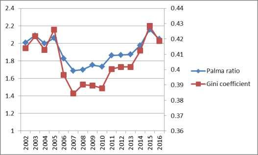
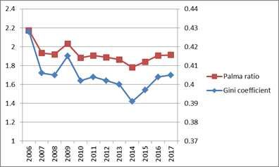
Gwithin= ( )GiniNUTS-1 ( Equation, 3)
 
Given that;
GiniNUTS-1= Gini value for NUTS-1 region;
 
 = population share of each income class in group j.
 
 =the income share of each income class in group j.
 
Summing up, investigation of the data sets comprise of three main features, which are interpretations of
descriptive statistics, whilst considering proportional change in income deciles, defining outliers by means of
the Mahalanobis distance and RB and Gwithin analysis for mapping regional disparities that is suggested to
contribute towards income inequality concentration both on a national and regional level in Turkey.

4.1 Comparison of the Gini coefficient and the Palma ratio for Turkey

Taking into account both data sets (Povcal data, Turkstat) for Turkey, it is seen that the Palma ratio ranges from
2.17 to 1.68 in the period from 2002 to 2017. According to the 2016 figures of the Povcal data, the Palma ratio
for Turkey is 1.91, that is, the second highest value (after Chile) among OECD members, On a global scale,
based on figures of the Palma ratio (Palma, 2018), Turkey could be classified among the “medium-level
inequality” group.

For the 2002-2016 period (Povcal data) only the Palma ratio is found to be left (negative) skewed and for the
years between 2006-2017 (TurkStat data) both metrics are positively skewed with negligible outliers.9

Based on the TurkStat and Povcal data set, a comparison of the Gini coefficient and the Palma ratio for Turkey
is shown (see figure 1.1, 1.2). As seen from figure 1.1, both metrics have a tendency to decrease after the 2003
period especially in the period 2003-2006. In the Aftermath of 2013, a tendency to increase has been observed.
Briefly, it is possible to classify different tendencies in inequalities depending on sub-period of economic
growth tendencies of the Turkish economy. More importantly, it is striking that this trend of the Palma ratio is
overlapping with changes in the Gini coefficient.

 Figure1.1: Palma Ratio and Gini Coefficient Figure 1.2: Palma Ratio and Gini Coefficient
(Povcaldata,2002-2016) (Turkstat,2006-2017)

As it is shown from figure 1.1 and 1.2, changing trends both in the Palma ratio and Gini coefficient are
completely the same. Both the Gini coefficient and Palma ratio receive the maximum and the minimum values,
in the same years. Moreover, the correlation among two variables is found to be very strong (as it is seen in
figure 2.1 and 2.2). For the Povcal data set, this correlation is calculated as (0.9887) and the TurkStat data set as
(0.9984) at a 95% confidence level.

9
 Regarding the sample size graph box analysis has been considered but not included

 7

Figure 2.1: Correlation of Gini coefficient and Figure 2.2: Correlation of Gini coefficient and
Palma ratio(TurkStat, 2006-2017) Palma ratio(Povcal, 2002-2016)
 1.8 2 2.2 1.6 1.8 2 2.2
 2006
 .44
 2015
 .42 2005
 2009
 2003
 2016
 .42
 2007 2002
 2004
 2014
 2017
 2008
 2011
 2016
 gini 2010
 2012 Ginipov
 2013
 2015 .4 2013
 2012
 2011
 2006 .4
 2014
 20082009
 2010
 2007

 .38 .38
 2.2 2006 2.2 2015
 2003
 2016 2005
 2002
 2004
 2 2014
 2009

 2 Palma 2013
 2012
 2011
 palma
 2007 2006 ratio
 2008
 2017
 2011
 2016
 2012
 2010
 1.8 2009
 2010
 2013
 2015 2007 2008

 1.8 2014
 1.6
 .38 .4 .42 .38 .4 .42 .44

In addition to these, the rate of change (either increase or decrease for different periods) is more stationary for
the Gini coefficient rather than the Palma ratio10. When proportional change for both the Palma ratio and the
Gini coefficient with respect to the total mean income and GDP per capita were examined between the 2006-
2017 period; the Palma ratio is found to be more sensitive to changes (negative values for both metrics has been
calculated).11 Nevertheless the period covered by the Povcal data proportional change with respect to mean
income is found to be positive12, indicating temporary recovery in inequalities for a longer time period. As an
overall result it could be suggested that after the post 2001 period in spite of increase in total mean and GDP per
capita, recovery in inequality has been stationary. Moreover, when proportional change is examined annually,
both metrics have negative and positive values for the same period and during the crises period of 2008-2009,
sensitivity to changes in GDP per capita income is found to be higher for both coefficients.13

An evaluation of descriptive statistics also reveals that the Palma ratio has got 2 times higher standard deviation
and coefficient of variation values than the Gini coefficient that lead us to explore relevant income deciles(see
appendix). Hence, in the light of descriptive statistics and strong correlations between two variables, the
explanatory power of the Palma ratio, with respect to changes in income deciles, will be investigated in the
following sections.

4.2.Centripetal and Centrifugal deciles of Turkey
In this chapter, given the basic features and propositions of the Palma ratio, questions of whether the income
inequality is concentrated in “tails” and on the other hand, the proposition of the relative stability of the D5-D9
income deciles, will be examined for the TR level.

For the periods covered by TurkStat and the Povcal data set, the results are consistent with the proposition of the
Palma ratio, that is; half of the income is shared by middle deciles and the other half of the income is shared
among the tails. For both data sets, it is seen that D5-D9 shares do not fall below 50 percent. Moreover, this
tendency indicates that the share of middle deciles is the reverse mirror image of the tails (see Figure 3.1 and
3.2). When the sum of the tails (D1-D4 and D10) has the lower ratio, the middle deciles take higher ratios,
hence, it could be suggested that the tails and the middle deciles are substitutes of each other. For the period
covered by Povcal data, it is seen that D5-D9 deciles share increased between 2005 and 2008 (maximum value

10
 Rate of change for Gini coefficient is only (0.02) and for Palma ratio is (0.14) for Povcal data set period. For period
2006-2017 rate of change for Gini coefficient is calculated as (-0.057) and for Palma ratio it is (-0. 06).
11
 Change in Palma ratio with respect to mean income is (-0.027) and GDP per capita income is (-0.02). Change in Gini
coefficient with respect to mean income is ( -0.022) and GDP per capita income is (-0.027). Once more, correlation with
proportional change with Palma and Gini coefficient is found to be strong.
12
 For Palma ratio (0.02) and Gini coefficient (0.01).
13
 For 2002-2016 period relation between GDP per capita and Gini coeffiecient and Palma ratio is expected to have - U -
relationship.

 8

in 2008) and later on this trend had been reversed. In the period covered by TurkStat data, the share of D5-D9
deciles have the highest ratio in 2007, although this ratio has decreased in the following periods.

Figure 3.1 : Centripetal and Centrifugal deciles Figure 3.2 : Centripetal and Centrifugal deciles
of Turkey(Povcal ,2002-2016) of Turkey(TurkStat,2006-2017)

 54
 55

 52
 50

 50
 48
 45

 46
 2000 2005 2010 2015 2006 2008 2010 2012 2014 2016
 years years

 d5d9 d10+d1d4 D1D4+D10 d5d9

Focusing on tails for both of the data sets’ periods, it is seen that the lowest D10 share also means the highest
D1-D4 share. When D10 has maximum value (2002, 2006), both D1-D4 and D5-D9 has a reverse trend. In the
period when D10 reaches the maximum level, the Palma rate is also the maximum.

For the Palma ratio covered by the Turkstat data period, the correlation between D1-D4 is found to be stronger
(-0.95) than the correlation with D10 income deciles (0.85). On the other hand, the Povcal data set correlation
between the Palma ratio and D1-D4 is (-0.9492) and the correlation with the Palma ratio and D10 is stronger
(0.9766).

However, one differing result for both data sets is with regards to the correlation between D5-D9 and D1-D4.
Relatively, a lower correlation for D5-D9 and D1-D4 income deciles is noteworthy and the correlation between
D5-D9 and D10 is found to be stronger and negative. Moreover, components of the Palma ratio have a stronger
tendency to change against the Gini coefficient compared to middle income deciles and the correlation between
the middle deciles and the Gini coefficient is found to be weaker.14 Including the fact that the D10 income decile
has a negative and high correlation value with middle deciles, it could be suggested that trends in D10 squeeze
the middle deciles as well.

According to the descriptive statistics, when the standard deviation and coefficient of variation values are taken
into consideration, one of the specific features that stands out (for both data sets) is the higher standard deviation
and range values for the D10 decile compared to the others. According to the Povcal data descriptive statistics,
values for D10 are approximately 2 times higher than the period covered by the TurkStat data set. It is observed
that D10 showed more variation in the period between 2002-2016.

As one of components of “tails”, D1-D4 income deciles trend of change differs according to the covered period
in both data sets whereas D5-D9 income deciles have relative stability. The Standard deviations of both income
groups is closer to each other between the years 2006 and 2017 (TurkStat data period). When the Povcal data set
period is taken into account, the standard deviation for middle deciles is found to be higher than the bottom
deciles. However, the coefficient of variation has the lowest values for D5-D9 in both data sets.

According to the data sets, after the aftermath of the 2008 crisis period, it is observed that the share of D10 has
increased its share compared to the others. Furthermore, for the last years covered by data sets, the trend to
increase in D10’s share has been observed. Moreover, when we look at the ventile income groups for the period
2006-2017 (Turkstat,2018), the differentiation “within the D10 income group” is notable. Consequently, V20
values are double those of V19 values. Furthermore, this figure has a 3 times higher standard deviation than

14
 Correlation is also examined for each income deciles and this prediction is confirmed.

 9

V19, that leads us to recall the importance of the Palma ratio V.2 to analyze the degree of concentration of the
inequalities as mentioned in Krozer's (2015).

Clearly, the different trend of income deciles could be interrupted with answers given to the question of who has
benefited from the increase in GDP per capita and the total mean income. In this case, due to the period covered
by the data sets, the results indicate that two different trends could be extrapolated (as mentioned in the previous
chapter).

Given that the Povcal data set covers the post 2001 period of Turkey, between the years 2002 and 2016 the
proportional change in the share of D1-D4 is found to be negative which is an opposite trend when compared to
other income groups and even for middle deciles this change is found to be the highest. Although for the period
between 2006-2017 the Palma premium indicates a different trend in income deciles15. Even proportional
change in the D1-D4 total mean with respect to the total mean income is found to be higher than the others.
Meanwhile, the proportional change in the middle deciles with respect to the total mean income and GDP per
capita, income is found to be weaker compared to the others even considering the proportional change in the
percentage share it is found to be negative and different from the others. Clearly, it could be suggested that
considering the sub-periods of GDP growth, the middle deciles share increased in the previous years but in the
aftermath this has decreased whereas the share of D10 has increased continuously and the recovery in the
bottom deciles has been temporary.

As a result, the centrifugal forces have been more volatile and relative stagnation of the centripetal forces has
been justified. On the other hand, among centrifugal forces, it could be suggested that evidently D10 income
group has the potential of squeezing other deciles. While focusing on the Palma ratio components and relevant
income groups, these facts could become more pronounced.

5.1 Palma ratio and Gini coefficient comparison on NUTS-1 level
For the post-2001 period, acceleration of the rate of GDP per capita has also lead to a limited level of
convergence among regions (Oz, 2017). For the period 2006-2017, regions real GDP per capita has increased to
above 2 percent. Even proportional change in GDP per capita income has been above Turkey’s average for
regions TRC, TRB, TR4 and TR1 (that is above 3 percent) compared to other regions and a lower increase has
been realized for TR9. TR1 apparently has the highest GDP per capita (approximately one third of TR’s GDP
per capita) income, whereas regions above the intra-regional mean of GDP per capita income are TR2,TR3,
TR4, TR5, TR6 and the others are below the intra-regional mean of GDP per capita income; TRA with lowest
GDP per capita mean. 16

Primarily when the total mean income of regions for the period of 2006-2017 is examined, heterogeneity of the
regions becomes apparent. Additionally, diversification of mean income levels for the regions is more explicit
compared with GDP per capita levels. Apparently, total mean income has doubled for all regions during that
period (only for TRC it is 3 percent) and TR9 region has achieved the lowest proportional change in total mean
income (this is relevant for proportional change in GDP per capita income).

15
 Palma preimum for 2006-2017 is (0.46). For Povcal data period it is negative.Average D10+ target for Turkey is about
8 percent.
16
 Due to limited space GDP per capita table has not been included.

 10

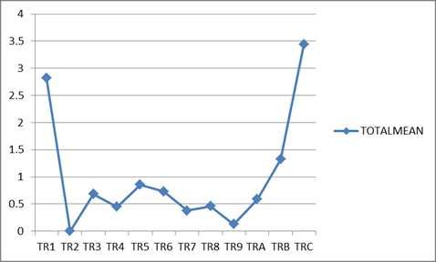
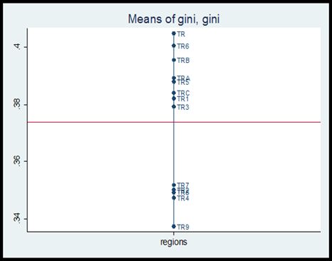
Figure 4.1 : Reel total mean income NUTS-1 Figure 4.2: Overall mean of RB analysis for total
level (2006-2017) mean income on NUTS-1 level(2006-2017)

Within this context, regions could be classified according to total mean values that are either above or below
TR’s mean income level (see fig.4). When the average of the mean income levels are taken into account, it is
found that, TR1 (highest mean income) and TRC (lowest mean income) regions indicate two opposite trends.
TR5, TR3, TR2 and TR4 regions own higher average mean income levels than the intra-regional average.
Besides, proximity of the average mean income level among TRA, TRB and TRC regions is more clear, having
said that these regions own the lowest average mean income levels compared to others.

Given that, according to ‘between’ group analysis for total mean income, ranking in descending order, TRC,
TR1, TRB, TR5, TR6, TR3 and TRA regions are found to have a higher contribution(above 0.5) to total mean
income inequality in Turkey17. (Equation, 2, Figure 4.2).

Given these facts, considering intra-regional distribution for the Gini coefficient and the Palma ratio, no outlier
figure has been detected. In addition to this, the skewness test for both metrics indicates normal distribution. 18
However while inter-regional figures have been examined, varieties in skewness have been observed.19

As can be seen from figure 5 and figure 6, the mean and range values taken by the Palma ratio over time reveal
the existence of intra-regional heterogeneity. For the period of 2006-2017, Turkey’s mean of the Palma ratio is
calculated as (1.92), while the intra-regional mean of the Palma ratio is (1.61). For the Gini coefficient, whilst
the mean of Turkey is (0.40), the intra-regional mean for the Gini coefficient has a lower value (0.37). While
TR6 region has the highest mean value (1.84) of the Palma ratio, TR2 region has the lowest mean value (1.42).
This tendency is observed to be similar with mean values of the Gini coefficient. As seen in figure 6, for both
the Palma ratio and the Gini coefficient, the regions that are above and below the intra-regional mean value are
completely overlapping, indicating the same trend relevantly for both ratios.

17
 For TR1(2.82), TR(0.001), TR3(0.68), TR4(0.44), TR5(0.85), TR6(0.733), TR7(0.37), TR8(0.45),
TRA(0.58),TRB(1.32),TRC(3.43).
18
 Based on graph box analysis on regional level within regions, TR1, TR3, TR4 and TR7 have outlier figure for Palma
ratio but intra-regional values have no outliers.For Gini coefficient also, outlier figures has been observed for TR1,
TR3,TR4, TR6,TR7,TRA regions.
19
 Only for Palma ratio, TR1 TR3 and TR7 have kurtosis values above 4.

 11

Figure 5: Palma ratio and Palma mean on regional level (TurkStat, 2016-2017)

 2.5
 2
 1.5
 1
 TR TR1 TR2 TR3 TR4 TR5 TR6 TR7 TR8 TR9 TRA TRB TRC
 regions

 Palma Palma_mean

Accordingly, when the Palma ratio’s mean values are taken into consideration, it is possible to mention three
main trends on NUTS-1 regional level( see fig 6.1 and 6.2). Regions could be divided into sub-groups (almost
the same for the Gini coefficient’s mean value); a) regions relatively close to the TR mean and above the intra-
regional mean value (1.61), TR6 (1.84), TRB (1.80), TRA (1.76). b) regions above and proportionally closer to
the intra-regional mean, TRC (1.73), TR5 (1.73), TR1(1.72), TR3 (1.67) c) regions below the intra-regional
mean value, TR9 (1.35), TR2 (1.41), TR4 (1.43) TR8 (1.43) TR7 (1.44). 20

Figure 6.1 and 6.2 : Means of Palma ratio and Gini coefficient (TurkStat, 2016-2017).

As a result of chart outlying mean values (fig. 6) and Mahalanobis distance calculation (Eq.1 , fig. 7) ,
overlapping trends between the Palma ratio and the Gini coefficient is clearly observed. Beyond that, the
regions away from TR are found to be the regions where the Palma ratio is lower, while the regions close to TR
are found to be the regions where this ratio is higher. Furthermore as seen in figure 7, regions that are closer to
TR’s values also contribute more to the total mean income inequality (see figure 5) and their Palma ratio mean
is found to be above the intra-regional mean.

20
 For this case I prefer to include TR values as well to make a comparison, when TR values is omitted ranking of NUTS-1
regions do not change. Just red lines (intra-regional mean) level changes.

 12

Figure 7: Mahalanobis distance for Palma ratio and Gini coefficient (NUTS-1,TurkStat,2016-2017)

Furthermore, as seen from figure 8, the intra-regional correlation between the Gini coefficient and the Palma
ratio is found to be strong (0.98) at 95% confidence interval, whereas the inter-regional correlation except the
TRC (0.6920) and TR6 (0.8224) regions indicates a strong correlation similar to intra-regional correlation
figures. As a consequence of the given results, the question of why a different trend has occurred in the TRC
and TR6 regions will be discussed in the following section.
 Figure 8: Correlation of Gini coefficient and Palma ratio( NUTS- 1 level, TurkStat, 2016-2017)
 1 1.5 2 2.5
 TR1 .45
 TRA
 TRB
 TR3
 TR6
 TR6
 TRB
 TRB
 TR5
 TRCTR1
 TRCTR5
 TRA
 TRBTR6
 TRA
 TRB
 TRA
 TR6
 TR6
 TR5
 TRA
 TR6
 TR6 TRA
 TRB
 TR6TR6
 TR1
 TR3
 TRC
 TR5
 TR5
 TR7
 TRC
 TR5
 TRA
 TR4
 TR1
 TR4
 TRA .4
 TRB
 TR6
 TR3
 TRB
 TRB
 TR5
 TR1
 TRATR6
 TR3
 TRATR8
 TR3
 TRB
 TRC
 TRC
 TR5
 TR9
 TR3
 TRC
 TR1
 TR5
 TRB
 TR1
 TR8
 TR5
 TR5
 TRBTR2
 TR1
 TR3
 TRC
 gini TR2
 TR4
 TR5
 TR1
 TR7
 TR8
 TR2
 TR9
 TR2
 TR3
 TR1
 TR7
 TR1
 TR2
 TR3
 TR7
 TR8
 TR9
 TRC
 TR3
 TRC
 TR7
 TR2
 TR9
 TR7
 TRA
 TR2
 TR2
 TR8
 TR9
 TR1
 TR8
 TR4
 TR7
 TR7
 TR4
 TR4
 TR8
 TR8 .35
 TR7
 TR4
 TR8
 TR2
 TR4
 TR8
 TR4
 TR8
 TR7
 TR2
 TR9
 TR2
 TR8
 TR4
 TR7
 TR9
 TR9
 TR4
 TR9
 TRA
 TR4
 TR2
 TR9
 TR9
 TR9

 .3
 2.5
 TR1
 TRA
 TRB
 TR3
 TR6
 TR6
 TRB
 TR1
 TR5
 TRB
 2 TRC TR6
 TRC
 TR6
 TRA
 TRA
 TR5
 TR6
 TRA
 TRB
 TRA
 TRB
 TR6
 TR6
 TR5
 TR3
 TR5
 TRC
 TR4
 TR5TRC
 TR1
 TRA
 TRC
 TR7
 TR4
 TR5
 TR6
 TRB
 TR1
 TR6
 TRA
 TRA
 TR3
 TR6
 TRB
 TR1
 TR5
 TR8
 TRB
 TR3
 TR5
 TR3
 TRC
 TR6
 TRB
 TRC
 TR9
 TR1 Palma
 TR1
 TR1 TRA
 TR3
 TRC
 TR2
 TRB
 TR5TRA
 TRC
 TR8TR5
 TR8
 TR3
 TR1
 TR4
 TR1
 TR7
 TRB
 TR5
 TR9
 TR1
 TR3
 TR2
 TR8
 TR3
 TR9 TR5
 TR2
 TR7 TR6
 TR2
 TR9
 TR7
 TR7
 TRC
 TR3
 TR2
 TR2
 TR1TR7
 TRA
 TR2
 1.5 TR4
 TR4
 TR4
 TR7
 TR8
 TR4
 TR7
 TR7
 TR8
 TR2
 TR8
 TR9
 TR8
 TR8
 TR4
 TR4TR8
 TR7
 TR2
 TR2
 TR9TR7
 TR4
 TR8
 TR4
 TR9TR8
 TR4
 TR9
 TR7
 TR2
 TR9
 TRA
 TR2
 TR9
 TR9
 TR9

 1
 .3 .35 .4 .45

While considering inter-regional21 and intra-regional range values for both metrics once more, the
heterogeneous structure of income inequality is clarified. The inter-regional difference between maximum and
minimum range values for the Gini coefficient is (2) times higher, while this figure is (2.5) times higher for the
Palma ratio. Regions having the highest (TRA, TR1) and the lowest range (TRC) values for both metrics are
overlapping.

On the other hand, the standard deviation and coefficient of variation values for the Palma ratio are found to be
higher than the Gini coefficient’s. One of the most prominent features of the descriptive statistics is about the
coefficient of variation of the Palma ratio that indicates a higher rate compared with other income groups.

Given the mean, range, standard deviation and coefficient of variance values for the Palma ratio, changes in
TRC and TR2 region is found to be more stationary while TRA and TR1 regions indicate a higher level of
volatility compared with other regions. Arranging the mean of standard deviation of regions also indicates an
overlapping tendency with the Palma ratio and the Gini coefficient, whereas TRA and TR1 are the regions with
the highest standard deviation for both metrics, and regions with the lowest standard deviation (TRC, TR2) for
the Palma ratio also have a lower standard deviation.

When proportional change with respect to mean income and GDP per capita income is considered, the Palma
ratio is found to be more sensitive compared to the Gini coefficient for NUTS-1 level as well. For the TR1 and
TR2 regions, proportional change for both metrics is found to be positive, which is different from other regions
21
 See Appendix.

 13

and TR. Additionally, sensitivity to changes in the Palma ratio, with respect to total mean income, reaches its
highest value in TR1 and TR2. The negative trend with highest sensitivity compared to other regions is relevant
for TR3. As a result it could be suggested that the increasing trend in GDP per capita and total mean income
became a determinant in TR1 and TR2 regions and the opposite for TR3. This could be interpreted as
amendatory. Hence, the Palma premium for TR1 and TR2 is found to be negative22 (different from other
regions) and the highest Palma premium ratio belongs to TR3 region.23

Briefly, the overlapping trend of the Palma ratio with respect to the Gini coefficient is found to be strong,
meanwhile, regions with a higher Palma ratio are found to contribute to total inequality more. Regarding the
evaluation of both of the metric’s estimations, outliers could be interrupted; so, for a deeper analysis of income
inequality, concentration, centripetal and centrifugal forces will be investigated.

5.1 Centripetal and Centrifugal forces on NUTS-1 level

For the period 2006-2017, dispersion of the Palma ratio components and the middle -income deciles reveals a
more complex picture in terms of inter and intra regional income inequality. Regarding this complex picture this
chapter aims to clarify the basic facts with regards to the trend of dispersion in income groups and aims to set up
linkages with trends of change in the Palma ratio and the Gini coefficient. Primarily, for all three income
groups, on an intra-regional level, the existence of outlier figures are insignificant. Although on an inter-regional
level, outliers for all income groups exist but only a few, so descriptive statistics would be utilized.

As seen in figure 10 (see appendix), the mean values for the centrifugal forces vary differently from TR’s mean
values. Although the mean values for the centripetal forces indicate a more homogenous income distribution.
Remarkably, due to the distribution of the centrifugal and centripetal forces “two separate segments” exist. The
Mahalanobis distance calculations for income groups percentage shares also confirm this suggestion (see fig. 9,
Eq.1). The proximity and homogeneity of the regions on the basis of D5-D9 share of TR’s is evident, although
the values for the centrifugal deciles indicate a more diversified structure. Even for the bottom deciles,
dispersion seems to be more diversified according to TR’s.

 Figure 9: Mahalanobis Distance for Income Deciles NUTS-1 level(% shares,2006-2014)

When the intra-regional mean values of the D1-D4 and the D10 income deciles are taken into consideration, it
is seen that the regions below the intra-regional mean and the regions remaining above are displaced, but there
is no one-to-one overlap. The intra-regional mean value for D10 is calculated to be below TR’s mean, while D1-
D4 regional mean value is found to be above TR’s mean.

22
 Palma premium; TR1(-1.17), TR2(-0.45)
23
 Palma premium;
TR3(1.04)TR4(0.75)TR50.69)TR6(0.80)TR7(0.094)TR8(0.69)TR9(0.78)TRA(1.04)TRB(0.69)TRB(0.81)TRC(0.81)

 14

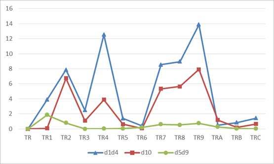
Figure 10 : Centripetal deciles of NUTS-1 Level(TurkStat,2016-2017)
 Means of D10, D10 Means of d1d4, d1d4
32

 20
 TR9
 TR4
 TR
 TR1
 TR6
31

 TRB TR8
 TR7
 TR2

 19
 TRC
 TR5
30

 TR3
 TRA
 TR1

 18
 TR3
 29

 TR5
 TRC
 TRB
 TR4 TRA

 17
 TR6
 28

 TR7
 TR8

 TR2 TR
 27

 16
 TR9

 state state

For D10, TR6(31.34) has the closest mean to TR, while the lowest mean value belongs to TR9 (26.79). The TR9
region with the lowest Palma ratio also has the lowest mean value for D10 and the highest mean value for D1-
D4 (17.10). The regions with the lowest D10 mean are found to be the regions with the lowest Palma ratio and
Gini coefficient mean. Adding that region (TR6), with the highest mean values of D10 has also the highest mean
value for the Palma ratio.

In addition, considering the regional mean values of the Gini coefficient, the regions with the highest D10 are
also found to be the regions with the highest Gini coefficient and Palma ratio. For regions other than TR1, it is
possible to generalize that the Palma ratio is lower for the regions with the highest D1-D4 mean. In this context,
the TR1 region stands at a more distinct point than other regions.

On the other hand, both on an interregional level, the correlation between the Palma ratio and D10 is higher
(positive) than the correlation between the Palma ratio and D1-D4 (negative) for all regions (except TR3 and
TRC). Similarity between the regional mean levels and the correlation coefficient results indicate a strong
relationship between the Palma ratio and the D10 and even between the Gini coefficient and D10 deciles. The
difference in the correlation coefficient for TR6 and TRC regions (as stated above) is mainly related to the
correlation between the D10 and D1-D4 figures that stay out of the %95 confidence interval. In addition, the
D5-D9 correlation with both metrics is found to be weaker (negative) than others income groups.

High range values for the three income deciles which are also higher than the TR’s range values indicate intra-
regional inequalities. In particular, the D10 range value (13.72) is noticeable, while the middle deciles range
value is (9.2) and the bottom deciles range value is calculated as (6.87). However, the ranking of the standard
deviation and the coefficient of variation according to inter-regional income deciles, confirms relative
instability of D10. The Higher standard deviation and coefficient of variation values of D10 within regions also
indicates inter-regional inequalities.

The mapping of standard deviation for regions it could be suggested that regions with higher and lower
standard deviation for the D10 income group also have higher and lower standard deviations for the Palma ratio
and the Gini coefficient. Furthermore, considering the standard deviation ranking of regions overlapping with
the Palma ratio and the Gini coefficients is apparent. The highest standard deviation of the D10 income deciles
belongs to the TRA (2.41) and TR1 (2.40) regions, while the lowest standard deviation is calculated as the TRC
(0.92) region.

The regions with the highest standard deviation for D1-D4 are TRA (1.37), and with the lowest standard
deviation is TR6 (0.71), although lower standard deviation for bottom deciles indicates lower standard deviation
values for both metrics, in this case the overlapping trend is as apparent as D10 income groups.

Another fact about dispersion in income groups is related to the standard deviation of middle income groups,
where it is found to be higher than the standard deviation of the bottom deciles. TR1 has the highest (1.5) value

 15

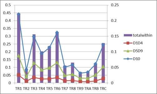
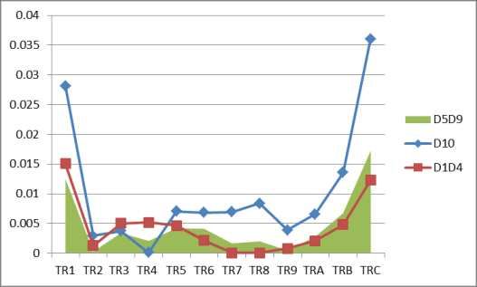
of standard deviation for middle deciles whereas TR3 has the lowest (0.51). Briefly arranging standard deviation
of middle deciles indicates another path different from the bottom and top income deciles.

When change with respect to mean income is investigated, the overall trend is found to be similar with TR’s
especially with TR1 and TR2 as mentioned in the previous section. This is due to the highest proportional
change in mean income of the region’s D10 deciles and contrary for lower values for D1-D4 and middle deciles.
As an overall result, proportional change in the middle income groups mean with respect to total mean income
is almost overlapping. Although, it is observed that proportional change in the bottom deciles has been higher in
other regions compared to other income groups. Considering proportional change with GDP per capita and the
percentage share of income groups, proportional change in share of D1-D4 is found to be more sensitive to
changes in GDP per capita income, whereas a mirror image relation among D10 and D1-D4 has been observed.
Another striking result is about proportional change in the middle income percentage share that is found to be
least sensitive to changes, except from TR1 and TR2.
Figure 11: Within group inequality of mean Figure 12: Between group analysis for total
income of relevant deciles mean income of relevant deciles

Under these given circumstances, regions with a higher Palma ratio and D10 mean income are found to be the
regions that have a higher contribution to ‘between’ regional inequalities, indicating the deterministic process in
explaining concentration of income inequality(Eq.2). Especially, the contribution to ‘between’ group inequality
in the case of D10 has been higher for TR1 and TRC regions and also higher in the case of D1-D4 income
groups.24 While regions with the lowest contribution to total inequality also have the lowest contribution to
between group inequality by means of D10(respectively TR2, TR9, TR4). In this case apart from TR4 , TR2 and
TR9 regions are found to have less contribution to between group inequality by means of D1-D4 income
groups.25

Apart from these, it should be underlined that (as it is seen from figure 11) regional income inequality exists not
only of differences in total income but differences in ‘within’ group inequality. Regarding ‘within’ group
inequality values(Eq.3), once more D10 is found to contribute more to inequality whereas the D1-D4 share has
the lowest contribution for each region. Jointly, regions with the lowest total ‘within’ values (TR2, TR9,TRA)
are found to have relatively lower ‘within’ values for D10. TR1, TR3, TR5, TR6 and TRC regions could be
classified among the regions with the highest ‘within’ inequality values. Adding to that, these regions have a
higher mean of the Gini coefficient and the Palma ratio, with D10 with a lower share of bottom deciles.26

24
 For D10 TR1(0.028), TRC(0.035) and for D1-D4 TR1(0.015) and TRC(0.12).
25
 For D10 TR2(0.002),TR4 (0.0001)TR9(0.003) and for D1-D4 TR2(0.0013) TR4(0.0051)TR9(0.007).
26
 For maximum values: TR1; D10(0.2), D1-D4(0.05), D5-D9(0.17), Totalwithin(0.44),TR3 ;D10(0.148),D1-4(0.035),D5-
D9(0.128), Totalwithin (0.31),TR6; D10(0.16),D1-D4(0.035),D5-D9(0.13),Totalwithin(0.33)TRC; D10(0.12),
D1-D4(0.028),D5-D9(0.10),Totalwithin(0.25).
For minimum values; TR9;D10(0.031),D1-D4(0.009), D5-D9(0.03),Totalwithin(0.07),TR2; D10(0.04),D1-D4(0.01),
D5-D9(0.040), Totalwithin(0.09).

 16