LATENT GOLD 5.0 UPGRADE MANUAL 1 - JEROEN K. VERMUNT AND JAY MAGIDSON
←
→
Page content transcription
If your browser does not render page correctly, please read the page content below
LATENT GOLD 5.0 UPGRADE MANUAL1

JEROEN K. VERMUNT AND JAY MAGIDSON

1
 This document should be cited as: Vermunt, J.K., and Magidson, J. (2013). Latent GOLD 5.0 Upgrade Manual.
Belmont, MA: Statistical Innovations Inc.
TABLE OF CONTENTS

1. Introduction ........................................................................................................................................................ 3

2. Latent GOLD Basic ............................................................................................................................................... 4

    2.1 Improved computational speed and memory use........................................................................................ 4

    2.2 Three-step modeling ..................................................................................................................................... 5

        Performing a Step-Three analysis using the Variables tab ............................................................................. 7

        Options on the Model, Output, and Technical tab ......................................................................................... 8

        Output of a Step3 analysis.............................................................................................................................. 9

    2.3 Scoring ........................................................................................................................................................ 10

        Obtaining the scoring rule using the Variables tab ...................................................................................... 10

        Options on Model tab .................................................................................................................................. 11

        Options on Output and Technical tab .......................................................................................................... 12

        Scoring output .............................................................................................................................................. 13

    2.4 New output ................................................................................................................................................. 13

    2.5 Data handling and validation ...................................................................................................................... 14

        Selecting records for the analysis ................................................................................................................. 14

        Holding out cases or replications for validation ........................................................................................... 14

        Keep option .................................................................................................................................................. 15

3. Latent GOLD Advanced ..................................................................................................................................... 16

    3.1 Latent Markov (latent transition) modeling ............................................................................................... 16

        Data organization ......................................................................................................................................... 16

        Defining a latent Markov model: Variables tab ............................................................................................ 17

        Covariates: Variables and Model tabs .......................................................................................................... 18

        Direct effects: Residuals tab ......................................................................................................................... 19

        Additional modeling options: Advanced tab ................................................................................................ 20

        Technical tab ................................................................................................................................................ 21

        Output in Markov ......................................................................................................................................... 21

    3.2 Other changes ............................................................................................................................................. 22

                                                                                    1
4. LG-Syntax .......................................................................................................................................................... 23
4.1 Log-linear scale models............................................................................................................................... 23
4.2 Continuous-time latent Markov models ..................................................................................................... 24
Model specification ...................................................................................................................................... 24
Output .......................................................................................................................................................... 25
4.3 Step-Three modeling .................................................................................................................................. 25
4.4 Gamma, beta, and von Mises models......................................................................................................... 27
4.5 Parameter specification options ................................................................................................................. 27
4.6 New output ................................................................................................................................................. 28
Statistics ....................................................................................................................................................... 28
Standard errors ............................................................................................................................................ 28
BVRs.............................................................................................................................................................. 29
Score tests and expected parameter changes (EPCs) .................................................................................. 29
Validation and holdout options .................................................................................................................... 29
Profile Graph ................................................................................................................................................ 30
Profile-longitudinal ....................................................................................................................................... 30
Monte Carlo options .................................................................................................................................... 30
User defined Wald tests ............................................................................................................................... 30
Power computation for Wald tests .............................................................................................................. 31
Ignore dependent variable(s) or knownclass in classification ...................................................................... 31
Options for writing output to files................................................................................................................ 31
References ............................................................................................................................................................ 33
21. INTRODUCTION
This manual describes the new features implemented in Latent GOLD 5.0 compared to versions 4.0 and 4.5.
Important changes are implemented in each of the three Latent GOLD modules -- Basic, Advanced and Syntax.
In this upgrade manual, we describe these changes in separate chapters for these three modules. Each chapter
starts with a short description of the functionalities of the module concerned and with an overview of the main
new features in version 5.0. Subsequently, all new features are described in detail.
Accompanying to this upgrade manual, the following additional information on Latent GOLD 5.0 is available:
Examples illustrating the new features in the GUI Examples and Syntax Examples menu entries of the
Help menu.
An updated Technical Guide for Latent GOLD 5.0 providing technical details and complete references.
An updated Manual for LG-Syntax 5.0.
Tutorials on step-three modeling, scoring, and Markov modeling.
32. LATENT GOLD BASIC
Latent GOLD 4.5 Basic consists of three point-and-click submodules, Cluster, DFactor, and Regression. Cluster is
used for clustering applications with a single nominal latent variable and multiple response variables. DFactor is
used to define models with multiple dichotomous or ordinal latent variables. Regression is used for mixture
regression modeling with a repeated univariate response variable. These functionalities remain unchanged in
Latent GOLD 5.0.
The primary new features in Latent GOLD 5.0 Basic are:
Major speed improvement by parallel computing; that is, by making use of the multiple processors
available in modern computers. There are also minor speed gains at stages of the data preparation,
parameter estimation, and output preparation, as well as efficiency gains in memory use affecting
mainly models for large data sets.
A procedure for bias adjusted 3-step latent class analysis for further analysis of latent classes with
external variables -- covariates or dependent variables / distal outcomes -- as proposed by Vermunt
(2010a), Gudicha and Vermunt (2013), and Bakk, Tekle, and Vermunt (2013). This is implemented in a
new point-and-click submodule called Step3.
A procedure for computing a scoring equation that can be used to classify new observations outside
Latent GOLD. This is included as one of the options in new Step3 submodule.
Various output extensions, including expanded chi-squared, log-likelihood, and classification statistics,
bivariate residuals for Regression models, bootstrap p-values for all chi-squared goodness-of-fit
statistics and for bivariate residuals, and Estimated Values for Cluster and DFactor models.
An option to select a subset of observations for the analysis and possibly use the remaining
observations for validation purposes (holdout cases or holdout replications) and an option to select
variables not used in the analysis for inclusion in the classification/prediction output data file.
2.1 IMPROVED COMPUTATIONAL SPEED AND MEMORY USE
An important improvement in Latent GOLD 5.0 is the use of parallel processing. This is achieved by running a
model using multiple threads, where the (maximum) number of threads can be specified by the user. The
default setting is that the number of threads is automatically set equal to the number of available processors
(cores).
Latent GOLD 5.0 uses two different types of parallelizations for its computations. The first involves distributing
multiple estimation runs of the same model across the available processors. This is what happens in the
starting values and the bootstrap procedures, where the multiple runs concern the different start sets and the
bootstrap replications, respectively. This type of parallelization speeds up computations by a factor close to the
number of available processors.
The second type of parallelization involves performing parts of the computations of a single estimation run in
parallel for portions of the data set, and subsequently combining (typically adding up) the obtained
information. This is used in the E step of the EM iterations and in the computation of the derivatives for the
Newton-Raphson iterations and the standard errors estimation. This will speed up the estimation in larger
problems (large data sets, models with many parameters, and/or models with many latent classes), where the
faster computations outweigh the additional “administration” of creating the threads and combining their
results.
4The Technical tab contains a new option “Threads” (see Figure 1). Here one can set the maximum number of
threads to be used by Latent GOLD. The default is “all”, implying that the maximum number of threads is set to
equal the number of processors available on the machine.
Figure 1. Technical tab with new option Threads and changed Start Values setting
Compared to Latent GOLD 4.0 and 4.5, we also slightly changed the default settings for the random starting
values procedure to make local maxima less likely. The number of start sets is increased from 10 to 16 (see
Figure 1), a multiplier of 2, 4, and 8. This means that some of the speed improvement is used for an
improvement in the starting value procedure. With 4 threads, the initial iterations for 16 starting sets will run
2.5 times faster than Latent GOLD 4.5 with 10 starting sets. After this, twice the number of initial iterations is
performed for 2 start sets (best 10% rounding up), but this does not require any additional computation time
because these are run in parallel.
Aside from the faster computation, various efficiency gains were achieved in the memory use, among others in
the storing of large design matrices in regression models. However, it should be noted that the use of multiple
threads increases the required amount of RAM memory. This is the result of the fact that each thread needs its
own versions of the internal arrays use in the computations. Thus, if the available RAM memory becomes a
problem, it is better to not use multiple threads or to set its maximum to a lower value.
2.2 THREE-STEP MODELING
After performing a latent class analysis, researchers often wish to investigate the relationship between class
membership and external variables. If these variables are predictors of the class membership, they can be
included in the LC model itself using the (active) covariate option. This is what we refer to as a one-step
approach. However, such a one-step approach has the disadvantage that cluster definitions may (slightly)
change when covariates are included. Also, it is difficult to perform an exploratory analysis with a large set of
covariates, and it is somewhat contra-intuitive to include external variables in the classification model.
5A popular alternative is a three-step approach in which one first estimates the latent class model of interest
(step 1), then assigns individuals to latent classes using their posterior class membership probabilities (step 2),
and subsequently investigates the association between the assigned class memberships and external variables,
say using a standard logistic regression analysis, a cross-tabulation, or an ANOVA (step 3). The main
disadvantage of such an (unadjusted) three-step analysis is that it yields downward biased estimates of the
association with the external variables of interest. This occurs because classification errors are introduced
when assigning individuals to latent classes (in step 2; see Bolck, Croon, and Hagenaars, 2004).
The new Step3 submodule resolves this bias problem by implementing the adjusted step-three analysis
procedures proposed by Vermunt (2010a) and Bakk, Tekle, and Vermunt (2013). These adjustments are based
on the fact that when assigning individuals to latent classes (in step 2), we can also obtain an estimate of the
number of classification errors, which is basically the information reported in the Latent GOLD classification
table(s). That is, since we know the amount classification errors, we can correct for it in the step-three analysis.
The two available classification methods are modal and proportional class assignment. Modal classification
means that individuals are assigned to the class with the largest posterior membership probability. This is what
one will usually do if one wishes to use the assigned class memberships for subsequent analysis with outside
Latent GOLD. Proportional assignment means that individuals are treated as belonging to each of the classes
with weights equal to the posterior membership probabilities. Proportional assignment (without bias-
adjustment) is what is also used to get the ProbMeans and Profile output for inactive covariates.
The two adjustment methods are the maximum likelihood (ML) step-three analysis proposed by Vermunt
(2010a) and a generalized version of the weighted step-three approach proposed by Bolck, Croon, and
Hagenaars (2004), which we refer to as the BCH adjustment. Technical details on the ML and BCH correction
methods, which can be applied with either modal or proportional class assignment, can be found in the above
references and in the Technical Guide.
The Step3 model can be used with external variables predicting the class membership (Covariate option) or
with external variables which are predicted by the class membership (Dependent option). These two types of
external variables are also referred to as concomitant variables and distal outcomes, respectively. It should be
noted that Step3-Covariate yields a multivariate analysis in which all covariates enter simultaneously in the
logistic regression model for the latent classes. Step3-Dependent yields a separate bivariate analysis for each
dependent variable, which is similar to cross-tabulations (for categorical variables) and ANOVAs (for continuous
variables). As in the other submodules, dependent variables can be specified to be ordinal, nominal,
continuous, count, or binomial count.
6Figure 2. ClassPred tab with the new option Keep
The utilization of three-step modeling in Latent GOLD proceeds as follows. One first builds a latent class model
in the ordinary way. After the final model is selected, one requests classification to a file (on the ClassPred tab;
see Figure 2), specifying that the external variables to be used in the step-three analysis are also added to the
output file (using the new Keep option). The step-three analysis is then done with the Step3 submodule using
the classification output data file.
PERFORMING A STEP-THREE ANALYSIS USING THE VARIABLES TAB
After opening the data file containing the classification information and the external variables, one selects
Step3 from the Model menu (see Figure 3).
Performing an adjusted step-three analysis proceeds as follows:
1) Set the type of Analysis (Covariate or Dependent), the type of Classification (Proportional or Modal),
and the type of Adjustment (ML, BCH, or None) (see right bottom of Figure 3Figure 4);
2) Move the posterior class membership probabilities from the data file into the box called Posteriors
(see right upper part of Figure 3);
3) Move the external variables into the box which, depending on the Analysis type, is called either
Covariates or Dependents, and set their scale types in the usual way;
1) Optionally, use Case Weights, specify the Select option, and/or use the Survey options (with Advanced
only), and change Model, Output, and Technical settings if desired.
4) Estimate the specified model.
7Figure 3. Step3 Variables Tab with USDID demo data
The default setting is Proportional classification with ML adjustment. In simulation studies, this method has
proven to perform best with covariates and with ordinal and nominal dependent variables. With dependent
variables which are continuous, count, or binomial count, the ML method may not work well when the
distributional assumptions are violated (Bakk and Vermunt, 2013). It is therefore advised to use the more
robust BCH adjustment in such cases. When using ML with such scale types, the program will give the warning
“The BCH method is preferred with Continuous, Count or Binomial Count variables”.
The Select option, which is new in Latent GOLD 5.0 Basic, will be discussed in more detail below. But one of its
specific uses in a step-three analysis should be mentioned here. If a LC Regression analysis with multiple
replications per case was performed in a step one analysis, the classification file will contain multiple records
with identical classification information. In the analysis in step three one should use only one of the replications
for each case. This can be achieved with a selection variable taking on a unique value for say the first record of
each case; for example, time=1 in a longitudinal application or one selected case per group in a two-level
application (Bennink, Croon, and Vermunt, 2013).
OPTIONS ON THE MODEL, OUTPUT, AND TECHNICAL TAB
The Model tab contains an option for including quadratic and interaction terms and missing values dummies in
a step-three Covariate analysis. In a step-three Dependent analysis, one can change the setting for the error
variances of continuous dependent variables.
The output options are mostly the same as those of the other Latent GOLD Basic model, although somewhat
more limited because certain items are not relevant in a step-three analysis (such as bivariate residuals and
classification-posterior). The Standard Errors option requires special attention. As shown by Vermunt (2010a)
and Bakk, Oberski, and Vermunt (2013), in a step-three analysis using proportional classification and/or BCH
adjustment, it is necessary to use robust standard errors (to take into account that the analysis is done with
multiple weighted records per case). Therefore, “Robust” is the default and the “Standard” and “Fast” options
are not available.
8The options on the Technical tab are the same as those in the other submodules, except for the fact that
missing values “include indicators/dependent”, bootstrap, and continuous factor are not available.
OUTPUT OF A STEP3 ANALYSIS
The output of a Step3-Covariate analysis consists of chi-squared, log-likelihood, and classification statistics,
Parameters, Profile, Probmeans, EstimatedValues, and Classification-Model. Chi-squared and log-likelihood
statistics take on the usual meanings, and classification statistics are in fact ‘model’ classification statistics
since there are no indicators or dependent variables in the model. The Parameters output provides information
similar to “Model for Clusters” in Cluster models; that is, the parameters of the logistic regression model for
the clusters, as well as their SEs, z-values, and Wald tests. Profile and ProbMeans show the bivariate
association between covariates and clusters in two different directions -- covariate distribution/mean given
class and class distribution given covariate value -- as is also done in Cluster. EstimatedValues and
Classification-Model contain the same information; that is, the cluster membership probabilities for each
covariate pattern.
In Step3-Dependent, log-likelihood statistics are obtained as the sum of the log-likelihood values for the
separate bivariate analysis per dependent variable. Chi-squared and classification statistics are not meaningful
here, and therefore omitted. The Parameters output contains information similar to “Models for Indicators” in
Cluster models; that is, the intercepts, cluster effects, and error variances for each dependent variable, as well
as their SEs, z-values, and Wald tests. Profile gives the class-specific distributions and/or means of the
dependent variables. The same applies to EstimatedValues.
92.3 SCORING
Users performing a Cluster or DFactor analysis often desire a scoring rule that can be used to determine the
class membership of new observations (observations which were not used in the model building stage). Latent
GOLD Basic 5.0 provides a new tool for obtaining such a scoring rule; that is, an equation which yields the
posterior class membership probabilities based on a person’s scores on the indicators and covariates used in
the original Cluster or DFactor model.
It turns out that, as in linear discriminant analysis, the posterior classification probabilities are a perfect linear
logistic function of the variables used in to construct the Cluster or DFactor model. This implies that the scoring
equation can be obtained “afterwards” by performing a logistic regression analysis using the posterior class
membership probabilities as weights (see e.g., Magidson and Vermunt, 2005). In fact, the procedure to obtain
the scoring equation is equivalent to a step-three (covariate) analysis with proportional assignment and
without adjustment for classification errors (None option), and with the original variables used as covariates.
Because of this similarity to step-three modeling, the scoring option is implemented as part of the Step3
submodule.
The implementation of the Scoring option in Latent GOLD is as follows. One first builds a latent class Cluster or
DFactor model as usual. After the final model has been selected, one writes the posterior classification
information to a file (using the option on the ClassPred tab). The scoring rule is obtained with the Step3
submodule using the classification output data file.
OBTAINING THE SCORING RULE USING THE VARIABLES TAB
After opening the data file containing the classification information and the indicators and covariates used in
the original analysis, one selects Step3 from the Model menu.
Figure 4. Variables and tab of Step3 showing how to obtain the scoring equation for diabetes demo .
Subsequently, one follows these steps (see Figure 4):
101) Set the type of Analysis to ‘Scoring’;
2) More the posterior class membership probabilities into the box called Posteriors;
3) Move the indicators and the covariates used in the original analysis into the box called Variables;
4) Optionally, use Case Weights and/or specify the Select option, which in most situations are not
needed, and change Model, Output, and Technical settings if desired.
5) Estimate the specified model.
In standard situations, the L-squared goodness-of-fit statistic will equal 0, indicating that the posterior
probabilities are reproduced perfectly by the equation created with the selected variables. Note that when the
Bayes Constant for the Latent Variable (Technical tab) is larger than 0, the L-squared cannot become exactly 0,
but if it is close to 0 the scoring rule is still correct.
OPTIONS ON MODEL TAB
There are two situations in which the L-squared will clearly be larger than 0, indicating that additional terms are
needed to get the correct scoring rule. The first is connected to the specification of the Cluster/DFactor model.
If this model contained continuous indicators with class-specific error variances, their quadratic terms should
also be included in the scoring model, and if it contained continuous indicators with class-specific error
covariances, the corresponding interaction effects should also be included in the scoring model. These are well-
known results from quadratic discriminant analysis. In models with categorical indicators, interaction terms are
needed if class-specific direct effects between indicators were included (defining such models requires Syntax).
Quadratic and interaction terms can be added to the scoring equation on the Model tab (see Figure 5).
Figure 5. Model tab of Step3 showing how include quadratic and interaction effects in scoring equation for diabetes demo .
Another situation in which the L-squared will not equal 0 occurs with missing values (when using the Include All
option for Missing Values on the Technical tab). To get the correct scoring rule, the equation should contain
separate parameters for the missing values. This option can be activated on the Model tab, where it is called
Missing Value Dummies. A missing value dummy is a variable which is added to the scoring equation, taking the
value 1 if the variable it refers to is missing and 0 otherwise. It should be noted that the missing values
11themselves are handled in the standard way; that is, they are imputed with either the mean or the average
effect, depending on whether the variable is numeric or nominal (see Technical Guide). The advantage of the
Missing Value Dummies option (rather than excluding missing values) is that when scoring new observations,
missing values will automatically be handled appropriately.
Note that it is also possible to build a scoring equation which does not yield a perfect match with the posterior
class membership probabilities. That is, one could decide to exclude some indicators or to exclude quadratic
and/or interaction terms to simplify the scoring rule.
OPTIONS ON OUTPUT AND TECHNICAL TAB
Most Output options are standard, but one deserves special attention. It is possible to translate the scoring
equation into SPSS syntax or some more generic language (C code) that can easily be adapted for other
statistical packages. This information is written to a specified file (see Figure 6). The SPSS variant can directly be
used to classify observation within SPSS.
Figure 6. Output tab in the Step3 submodule to with diabetes demo .
Important Note: The scoring syntax yields .SPS or other commands that produce the posterior membership
probabilities based on the model variables in the format used in the final model. Therefore, the Scoring Syntax
should not be used when the final model is based on data that has been recoded with the ‘grouping’ or
‘uniform’ options within Latent GOLD.
One Technical option that needs special attention is the Bayes Constant for the Latent variable. As always,
setting this constant to a value larger than 0, will slightly smooth the parameter estimates. However, the
goodness-of-fit statistics will then no longer be exactly 0.
12Another important Technical option concerns the treatment of Missing Values. By default cases with missing
values are excluded. However, if you decide to retain cases with missing values in the scoring model (Include All
option), you should use Missing Values Dummies (see Model tab) to get the correct scoring equation.
SCORING OUTPUT
The goodness-of-fit statistics output will provide the most useful statistics information. The classification
statistics will take on the same values as in the original model, assuming that the scoring model fits perfectly.
The same applies to Profile and ProbMeans output.
The Parameters output contains the scoring equation in its logistic form. The reported SEs, z-values, and Wald
test do not have their standard meaning and will usually be ignored. However, one can use the Wald statistics
as relative measures indicating the importance of a specific variable compared to the other ones.
2.4 NEW OUTPUT
In this section we list the few new output items provided in Latent GOLD Basic. Their formulae are given in
Version 5.0 of the Technical Guide.
Goodness-of-fit statistics:
- SABIC(L-squared): sample size adjusted BIC, an information criterion similar to BIC but with log(N)
replaced by log((N+2)/24)
- Total BVR: the sum of the BVRs (bivariate residuals)
Log-likelihood statistics:
- SABIC(LL): sample size adjusted BIC, an information criterion similar to BIC but with log(N)
replaced by log((N+2)/24)
Classification Statistics:
- Classification Table(s) also in DFactor models
- Classification Table(s) for proportional classification (in addition to modal)
- Entropy (En)
- Classification Likelihood Criterion (CLC=2*CL)
- ICL-BIC (=BIC-2*En)
Bootstrap p-values and critical values at alpha=.05 for all goodness-of-statistics:
- L-squared, X-squared, Cressie-Read, and Dissimilarity index
- Total BVR
- Bivariate Residuals
Estimated Values also in Cluster and DFactor:
- (Joint) latent probabilities given covariates
- (Joint) indicator probabilities/means given latent variables and covariates
132.5 DATA HANDLING AND VALIDATION
Latent GOLD 5.0 Basic contains two new options which simplify data handling: the Select option on the
Variables tab and the Keep option on the ClassPred tab. The Select option can also be used for validation
purposes; that is, for holding out cases or replications from the analysis.
SELECTING RECORDS FOR THE ANALYSIS
The Select option makes it possible to select a subset of the records in the input file for the analysis to be
performed. The remaining non-selected records are ignored for estimation purposes. For example, this option
may be used to perform separate analyses for males and females, without the need of creating two separate
data files. Using this option requires moving the selection variable into the Select box (see Figure 7, performing
a Scan of the data file (Scan button), double clicking on the selection variable, and making sure that the right
categories are (un)checked (see Figure 7).
Figure 7. The variable ‘sex’ used in the ‘Select’ option and to perform an analysis for males only.
HOLDING OUT CASES OR REPLICATIONS FOR VALIDATION
The Select option can also be used for validation purposes. The analysis is performed with the selected subset
of records from the input file. However, after parameter estimation is completed, statistics are also computed
for the remaining (holdout) records. When the holdout records are holdout cases (see option “Unselected
Categories” in Figure 7), separate chi-squared, log-likelihood, classification, and predictions statistics are
provided for these cases. When the holdout records are holdout replications, which is possible only in
Regression, a separate set of prediction statistics is provided for the holdout replications.
It should be noted that the holdout option can not only be used for validation purposes, but also for scoring the
holdout records. That is, one can use a portion of the sample for parameter estimation, and obtain an output
file with classification and/or prediction information for all observations (including the holdout records).
14KEEP OPTION
The Keep option on the ClassPred tab (see Figure 8) makes it possible to create an output file not only
containing the classification/prediction information and the variables used in the analysis, but also any of the
other variables in the analyses (input) file. This means that it is no longer necessary to merge the Latent GOLD
classification/prediction output file with the original file prior to performing subsequent analyses, for example,
a step-three analysis.
Figure 8. Variables added to the output file using the ‘Keep’ option in the ClassPred tab
153. LATENT GOLD ADVANCED
The Latent GOLD 4.5 Advanced module makes it possible to use various advanced options in Cluster, DFactor,
and Regression models. These are options for dealing with complex sampling features in standard error
computation (Survey option), for defining models containing (also) continuous latent factors, and for defining
multilevel variants of the Latent GOLD Basic models.
The primary new features in Latent GOLD 5.0 Advanced are:
A new point-and-click submodule called Markov, which is a user-friendly tool for estimating a large
variety of latent Markov models, including models with multiple indicators of different scale types,
models with covariates, and mixture and mover-stayer models. An efficient (Baum-Welch or forward-
backward) algorithm is used, making it possible to deal with large numbers of states and time points.
Computational speed improvements, not only by the use of parallel computing, but also by the fact
that analytical instead of numerical second derivatives are now implemented for Markov and
multilevel models. This makes a major difference in the Newton-Raphson iterations and the
computation of standard errors computation in these models.
Various newly developed output: longitudinal bivariate residuals and longitudinal profile for Markov
models, and information criteria based on the number of groups and two-level bivariate residuals for
multilevel models
3.1 LATENT MARKOV (LATENT TRANSITION) MODELING
The most important new feature in Latent GOLD 5.0 Advanced concerns the submodule called Markov, which
allows estimating the most important types of latent Markov models. The latent Markov model is a popular
longitudinal data variant of the standard latent class model; it is in fact a latent class cluster model in which
individuals are allowed to switch between clusters across measurement occasions (Magidson, Vermunt, and
Tran, 2009; Vermunt, Tran, and Magidson, 2008; Vermunt, 2010b). The clusters are also called latent states,
and the model is also referred to as latent transition model.
Latent Markov modeling was already available in LG-Syntax 4.5. Because of its complexity, Markov modeling
with Syntax can be somewhat tedious, which is why we decided to implement these models in a more user-
friendly way. Although the Markov submodule allows setting up the model of interest without using Syntax,
behind the scene the program will generate the required Syntax, run the Syntax model, and display the Syntax
output. There are a few minor differences compared to using the Generate Syntax option and running the
model with LG-Syntax; the most important one is that similar to Cluster, DFactor, and Regression performed
with the point-and-click GUI, the categories of the latent variable(s) will always appear in the same order (from
large to small).
DATA ORGANIZATION
Before discussing the specification of latent Markov models, we need to discuss the data organization. Since
the time structure used for the model specification is derived from the data structure, if the data is not
organized correctly, the results obtained with Markov will be incorrect or even completely meaningless.
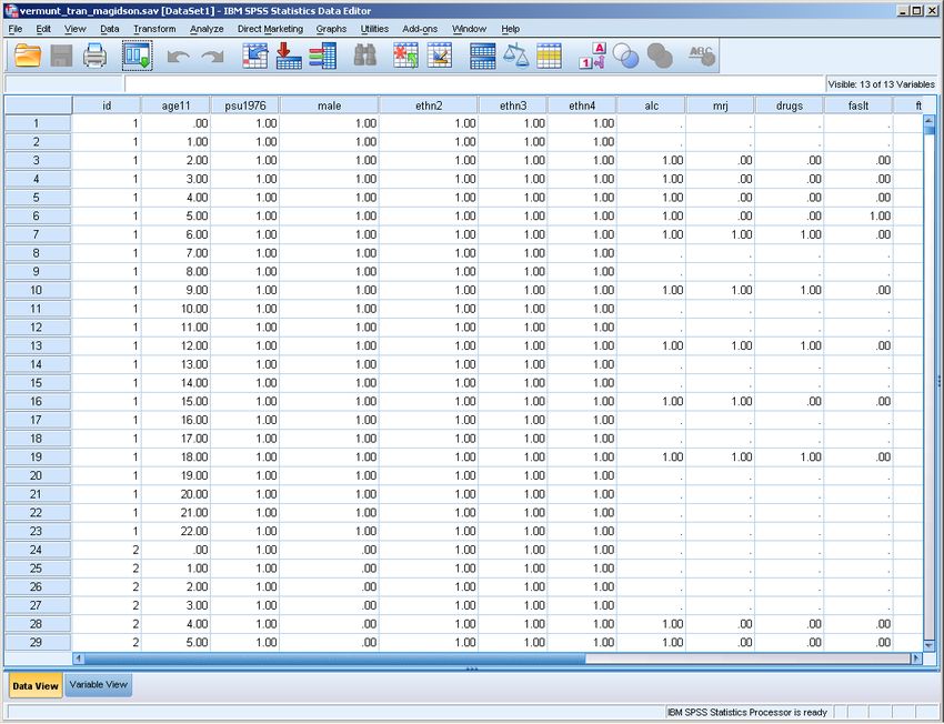
Markov assumes the data is in long format; that is, in the form of a person-period file (see Figure 9). More
specifically, it is assumed that the records of an individual case refer to equidistant discrete time points,
starting from the time point one wishes to treat as the initial time point until the last available measurement
for the person. Since the length of observational period may vary across cases, the total number of records
(time points) may differ across persons.
16In a Markov model, the first observation of a person is treated as the measurement at the initial time point
(t=0). Each next record corresponds to a next discrete measurement occasion. Thus, it is not allowed to skip
time points, for example, because no data are available for the time point concerned. Suppose the discrete
time unit in the Markov analysis is month (that is, one wishes to model monthly transitions). The data file
should then contain one record for each month until the last month for which one has a measurement for the
person concerned. If there is no information available at a particular intermediate month, one should insert a
record with missing values on the indicators. Vermunt, Tran, and Magidson (2008) provide detailed information
and an extended example on inserting records with missing data to get the required time structure.
The data file should contain a case id that can be used to connect the multiple records (time points) of a
person. Moreover, records should be sorted in ascending order on time within cases; that is, the order t=0, t=1,
t=2, etc. within case id’s.
In Markov models, it is important not to exclude cases with missing values, because otherwise the time
structure of the data set will be distorted. This implies that one should use the missing values setting “missing
includeall”, which is the default setting in Markov.
Figure 9. Long format data file.
DEFINING A LATENT MARKOV MODEL: VARIABLES TAB
A latent Markov model is in fact a Cluster model for longitudinal data. The model definition is therefore very
similar to the definition of a Cluster model. The only differences are that the nominal latent variable is called
“States” instead of “Clusters”, and that a case id has to be specified to connect the longitudinal measurements
of a case.
Specification of latent Markov model involves the following steps (see Figure 10):
Move the Indicators, and set their scale types;
17 Select a Case ID;
Specify the number (or a range) of States;
Estimate.
A latent Markov model contains three sets of parameters and their associated probabilities/means. These
concern the initial state (t=0) probabilities, the transition probabilities between time points t-1 and t (for t>0),
and state-specific distributions of the Indicators. The latter are, as in Cluster models, used to profile the latent
states.
Figure 10. Latent Markov Variables tab.
COVARIATES: VARIABLES AND MODEL TABS
As in the other Latent GOLD models, it is possible to include covariates in a Markov model. It is important to
distinguish two types of covariates: time-constant and time-varying covariates. Time-constant covariates can
be used in the model for the initial state probabilities and in the model for the transition probabilities. In
contrast, time-varying covariates can only be used in the model for the transition probabilities. On the Model
tab one can specify whether a covariate affects the initial states, the transitions, or both (see Figure 11).
An important time-varying covariate is time itself. A model in which the transition probabilities vary over time
is defined by including a time variable as a covariate affecting the transition probabilities. Time can be treated
as nominal, but it is also possible to define models with say linear, quadratic, cubic time effects on the
transition logits by making sure that the data file contains the appropriate time variables.
As in the other Latent GOLD models, covariates can be specified as inactive, which in a Markov model implies
that these will appear in the ProbMeans output. A special option specific to Markov models is the possibility of
using the categories of a selected covariate as time labels for the output (Covariate option Time Label).
18Figure 11. Latent Markov Model tab with the relevant covariates effects checked.
DIRECT EFFECTS: RESIDUALS TAB
As in Cluster model, it is possible to include direct effects (local dependencies) between indicators in the
model. It also possible to include direct effects of both time-constant and time-varying covariates on the
indicators.
Figure 12. Advanced tab of the Markov module
19ADDITIONAL MODELING OPTIONS: ADVANCED TAB
In addition to the complex sampling option, the Advanced tab contains other advanced modeling options
specifically for latent Markov models. These concern the use of Classes (in addition to States), the definition of
the States, and the specification of the Model for the Transition probabilities (see Figure 12).
CLASSES
The option Classes makes it possible to define mixture latent Markov models; that is, latent Markov models in
which the initial state and transition probabilities differ across latent classes. Specification of such models
simply involves increasing the number of Classes from 1 to a larger number. Note that the standard latent
Markov model is a 1-class model.
When checking the option Stayer, the first Class will be assumed to have transition probabilities equal to 0; that
is, to be a Stayer class. This option makes it possible to define mover-stayer models with any number of mover
classes.
When increasing the number of Classes from 1 to a higher number, various additional options become
available in the Model tab. These indicate whether Classes affect the Indicators directly, whether covariate
effects on the initial state and transition probabilities should vary across classes, and whether the class sizes
themselves are affected by (time-constant) covariates.
STATES
A second set of options refers to the specification for the latent States, which in the default specification are
modeled as Nominal. The option Ordinal implies that the states are modeled as a discrete factor (DFactor); that
is, as ordinal categories with fixed equidistant scores. The option Order-restricted is the same as Order-
restricted Clusters in Cluster models. It yields a model with monotonically increasing states as far as their
indicator distributions are concerned.
The option Perfect can be used to define manifest Markov models. When Perfect is selected, the States will be
defined to be perfectly related to the first nominal or ordinal indicator with the same number of categories as
the specified number of states. If no such indicator is available, an error message will be provided.
MODEL FOR TRANSITIONS
A third advanced option refers to the type of Model for the Transition probabilities. In the default setting, a
logit model is specified in which there are separate intercepts and covariate effect parameters for each
transition. This is achieved by conditioning these effects on the origin state (the state at t-1), and using dummy
coding for the state at t, but with a reference category that varies with the origin state. That is, the no
transition category serves are the reference category. We call this transition coding because the parameters
refer to the log odds of the making transition concerned versus staying in the same state.
The alternative specification involves using a standard logit model; that is, a multinomial logit model for the
state at time t containing an intercept term, an effect of the origin state (the state at t-1), and an effect for
each of the included covariates. With covariates, this model is more parsimonious because the covariate
effects on the destination state do not vary across origin states. Also in models with more than two Ordinal
states, this model will be slightly more restrictive because the origin-destination relationship is modeled with a
single (uniform association) parameter.
20TECHNICAL TAB
The technical settings are the same as those of the other Latent GOLD Basic modules, except for the one
concerning the treatment of Missing Values. As indicated above when discussing the data structure, in Markov
models one will typically use the Include All option because removing records with missing values will distort
the time structure. Include All is therefore the default setting.
OUTPUT IN MARKOV
The Output options are the same as in Cluster and Factor models. Before describing the content of the output
sections which are specific for Markov models, it should be noted that the latent States appear in the output in
three different ways: that is, as States, State[=0] and States[-1]. In this way, we refer to the state at time point t
(the state at a particular time point), at time point t=0 (the initial state), and at time point t-1 (the previous
time point), respectively.
Statistics are the same as in the Latent GOLD Basic modules, although classification information is provided for
both Classes and States.
The Parameters output contains the regression coefficients of the logit models for the initial state and
transition probabilities. Also the regression parameters and (co)variances for the indicators are provided.
Profile contains similar information as in Cluster and Factor models; that is, the Indicator distributions/means
for the different categories of the latent variables. Specific for Markov models is that one obtains the overall
State proportions (averaged over time points), as well as the overall transition probabilities (averaged over
classes and covariate patterns).
Profile-longitudinal is an output section which is specific to Markov models. As the standard Profile, it gives the
State- and Class-specific distributions/means of the indicators, but now per time point. This makes it possible to
see how the indicator distributions change over time. In addition, the overall predicted and observed
distributions/means are reported, making it possible to determine how well the model describes the overall
change pattern in the data. The Profile-longitudinal contains a new interactive graph (see Figure 13), which can
be modified with the plot control that pops up with a right click on the graph.
1.0
0.8
0.6
0.4
0.2
0.0
1
2
3
4
5
6
7
8
9
10
11
12
13
14
15
16
17
18
19
20
21
22
23
Time
St ate:1 Mea n(alc)
St ate:2 Mea n(alc)
St ate:3 Mea n(alc)
Ov erall Mea n(alc)
Observ ed Mean(alc)
Figure 13. Longitudinal-Plot with Predicted vs. Observed for each of 3 Indicators
21ProbMeans gives the same information as in other models. What may be of special interest is the output
associated with a time variable, which shows how the state distribution develops over time.
Similar to Regression models, Frequencies/Residuals will consist of multiple lines per data pattern. More
specifically, it will show the covariates and indicator values at each time point (with the time points denoted by
the internal variable “_timeid_” if no Time Label is specified), and the observed and estimated frequencies are
repeated across the multiple time points for the data pattern concerned.
Bivariate residuals provides the same BVRs for pairs of indicators as in Cluster and DFactor models, but also
three newly developed BVRs are available for Markov models. We call the latter Pearson chi-squared like
measures ‘longitudinal BVRs’. The three variants are BVR-time, BVR-lag1, and BVR-lag2. BVR-time quantifies
how well the time-specific distribution for the indicator concerned is fitted by the model. It is, in fact,
equivalent to the BVR obtained when using a nominal time variable as a covariate. BVR-lag1 and BVR-lag2
quantify the difference between the estimated and observed frequencies in the two-way cross-tabulation of
the indicator values at 1) t-1 and t and 2) t-2 and t, respectively. These BVRs indicate how well the first- and
second-order autocorrelations in the responses are picked up by the model.
Classification-Posterior and Classification-Model are similar to what is obtained in other models, except for the
fact that for the States one obtains a classification for each time point. With the option “Joint” (right click) one
also obtains the state probabilities 1) conditional on class, and 2) conditional on origin state and class.
EstimatedValues provides the model probabilities; that is, the class probabilities per covariate pattern, the
initial state probabilities for each covariate pattern and class combination, the destination state probabilities
for each covariate pattern, class, and origin state combination, and the conditional probabilities/means for the
indicators.
3.2 OTHER CHANGES
Another change in the Advanced module concerns the fact that analytical rather than numerical second
derivatives are available for latent Markov models and multilevel latent class models. Combined with the
parallel processing, this implies that the Newton-Raphson iterations and the computation of standard errors
will be much faster in these models. Actually, the numerical computation of second derivatives in earlier
version of Latent GOLD could slow down the estimation quite a bit in larger models. This will no longer occur in
version 5.0.
Latent GOLD implements various new statistics for multilevel models. These are forms of the BIC, CAIC, and
SABIC information criteria using the number of groups instead of the number of cases as the sample size
(Lukociene, Varriale and Vermunt, 2010; Lukociene and Vermunt, 2010), modal and proportional classification
tables for GClasses, and two types of newly developed BVRs (Nagelkerke, Oberski, and Vermunt, 2013). We
refer to the latter as two-level BVRs. One type is the BVR-group which is based on the groupid-indicator cross-
tabulations. It quantifies how well group differences in the indicator distributions are reproduced by the
specified model; that is, it quantifies the residual differences in responses between groups. The other type,
named BVR-pairs, is based on the cross-tabulation of the responses of all pairs of cases within groups. It
indicates how well the within-group associations are explained by the specified multilevel model, or shows the
residual dependence between cases within groups.
224. LG-SYNTAX
The LG-Syntax module allows one to specify a large variety of latent variable models. Models may contain
discrete and/or continuous latent variables and latent variables at multiple hierarchical levels, including
dynamic discrete latent variables for latent Markov modeling. The LG-Syntax module also contains options for
imposing parameter constraints and defining parameter starting values. Other features include Monte Carlo
simulation and multiple imputation tools.
The primary new features in LG-Syntax 5.0 are:
The possibility to include scale parameters in models for categorical response variables. These scale
parameters are modeled with a log-linear equation.
The possibility to define continuous-time latent Markov models in addition to discrete-time models.
A general tool for three-step latent class analysis, which allows defining a more general class of step-
three models than with the Step3 submodule, such as three-step variants of multilevel latent class
models, latent Markov models, and latent class models with multiple latent variables, and step-three
models containing both independent and dependent variables.
Three new types of regression models for dependent variables coming from gamma, beta, and von
Mises distributions. These can be used with continuous dependent variables which are nonnegative,
between 0 and 1, and circular, respectively.
New options for the model equations include the possibility to define cells weights (~wei), missing
value dummies for covariates (~mis), higher-order log-linear association terms between categorical
dependent variables, and starting values and fixed values in array form or in external files.
Various new output options, which include graphs for the Profile output, extended Monte Carlo
(bootstrap, MC study and power) options, extended validation and holdout options, various new types
of BVRs, score tests and expected parameter changes (EPCs), user-defined Wald tests, new types of
SEs, asymptotic power computations for Wald test, the option to ignore selected dependent variables
in the computation of the posterior class membership probabilities, and extended options for writing
output to text files.
It should be noted that these new options are also available in Choice models estimated with Syntax.
4.1 LOG-LINEAR SCALE MODELS
A new modeling feature is the possibility to include a scale factor in regression models for categorical response
variables; that is, in models for nominal and the various types of ordinal dependent variables. A scale factor is a
term by which all parameters in the regression model are multiplied, and which thus allows modeling
proportionality of parameter values across groups. The inverse of the scale factor is proportional to the
standard deviation of the error distribution when using the underlying latent variable interpretation of the
categorical response regression model concerned.
The scale factor is modeled by a log-linear equation, yielding a flexible approach for modeling its dependence
on latent and/or independent variables. It moreover guarantees that the scale factor remains non-negative. For
example, with two predictors z1 and z2, the scale factor model would have the following form exp(d1z1+d2z2).
Note that typically the intercept term will be excluded for identification purposes. Vermunt (2013) provides a
more formal description of these log-linear scale models, and Magidson and Vermunt (2007), and Magidson,
Thomas, and Vermunt (2009) present applications of latent class models with scale factors.
The scale model appears as one of the equations in the LG-Syntax equations section. The scale factor equation
is identifiable by the symbol “with the latent and independent variables at the right-hand side. All options available for regression equations
can also be used with scale factor equations, such as conditional effects, interactions, and parameter
constraints, except for most of the “~” parameter options. An example of a scale factor equation is:
responseOUTPUT
Most output is the same as in discrete-time latent Markov models. Below we discuss only the items which are
different in continuous time models.
The regression Parameters of the transition model are log-intensity rather than logit parameters.
Exponentiating these parameters yields the transition intensity parameters. The inverse of the sum of
transition intensities over the different destinations states yields the average length of stay in the origin state
concerned.
EstimatedValues contains the transition probabilities for the time intervals which occur in the sample. If you
wish to see the transition probabilities for another time interval, this can be obtained by adding a record to the
data for that time interval, with missing values for the dependent variables.
In the computation of the Profile and Profile-Longitudinal output, LG-Syntax does not take into account that
the measurements were obtained at unequal time intervals (so in fact treats them as equidistant discrete-time
data). The latent state proportions and the transition probabilities reported in Profile are averages across the
measurement occasions in the analyzed data set. Moreover, the time scale used in Profile-Longitudinal that of
a discrete time variable.
4.3 STEP-THREE MODELING
Latent GOLD 5.0 Basic contains a new Step3 modeling submodule. This analysis option is also available in LG-
Syntax 5.0, but can be used in a more general class of models. Defining a step-three analysis involves:
opening a data set containing the posterior classification probabilities from step 2,
specifying the step3 settings in the options section of the syntax,
defining the posteriors along with the latent variable(s) specification,
and setting up the remaining part of the model in the usual manner.
Let us first look at the translation of the Step3 GUI models into syntax as done automatically using the
‘generate syntax’ menu option. A Step3-Covariate model using proportional classification and the ML
adjustment is specified as follows:
options
step3 proportional ml;
output parameters standarderrors estimatedvalues;
variables
independent z1, z2, z3;
latent Cluster nominal posterior=(clu#1 clu#2 clu#3);
equations
ClusterYou can also read