On an integer-valued stochastic intensity model for time series of counts
←
→
Page content transcription
If your browser does not render page correctly, please read the page content below
Munich Personal RePEc Archive

On an integer-valued stochastic intensity
model for time series of counts

Aknouche, Abdelhakim and Dimitrakopoulos, Stefanos

USTHB and Qassim University, University of Leeds

1 January 2020

Online at https://mpra.ub.uni-muenchen.de/105406/
MPRA Paper No. 105406, posted 25 Jan 2021 16:59 UTC
On an integer-valued stochastic intensity model for time series of
                                                    counts
                       Abdelhakim Aknouche* and Stefanos Dimitrakopoulos1**
  *
      Faculty of Mathematics, University of Science and Technology Houari Boumediene (Algeria) and Qassim
                                            University (Saudi Arabia)
                                  **
                                     Economics Division, Leeds University, UK

                                                    Abstract

            We propose a broad class of count time series models, the mixed Poisson integer-valued stochas-
        tic intensity models. The proposed specification encompasses a wide range of conditional distri-
        butions of counts. We study its probabilistic structure and design Markov chain Monte Carlo
        algorithms for two cases; the Poisson and the negative binomial distributions. The methodology
        is applied to simulated data as well as to various data sets. Model comparison using marginal
        likelihoods and forecast evaluation using point and density forecasts are also considered.

            Keywords: Markov chain Monte Carlo, mixed Poisson, parameter-driven models

            JEL CODE: C00, C10, C11, C13, C22

   1
     Correspondence to: Stefanos Dimitrakopoulos, Economics Division, Leeds University Business School, Leeds Uni-
versity, UK, E-mail: s.dimitrakopoulos@leeds.ac.uk, Tel: +44(0) 113 3435637. The present version of the paper
is a substantial improvement of the MPRA paper (MPRA:91962) titled: “Integer-valued stochastic
volatility”.

                                                        1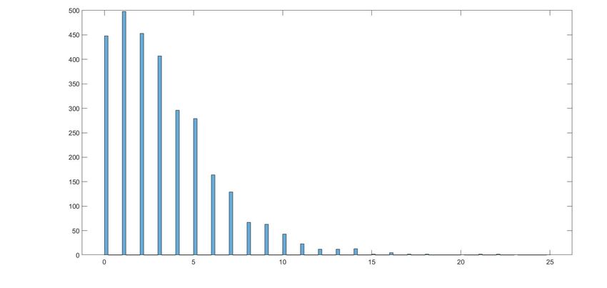
1     Introduction
Nowadays, time series count data models have a wide range of applications in many fields (finance,
economics, environmental and social sciences). The analysis of this type of models is still an active
area (Davis et al., 2016; Weiß, 2017), as numerous models and methods have been proposed to account
for the main characteristics of count time series (such as, overdispersion, underdispersion, and excess
of zeros).
    Many count time series models are often related to the Poisson process with a given paramet-
ric intensity. Following the general terminology by Cox (1981), these models can be classified into
observation-driven and parameter-driven, depending on whether the dependence structure of counts
is induced by an observed or a latent process, respectively.
    One way of introducing serial correlation in count time series is through a dynamic equation
for the intensity parameter, which may evolve according to an observed or an unobserved process.
Observation-driven models of counts with a dynamic specification for the intensity parameter are
mainly represented by integer-valued generalized autoregressive conditional heteroscedastic processes
(IN GARCH). This paper deals with the theory and inference of parameter-driven models of counts
with a dynamic specification for the intensity parameter.
    As is well known, IN GARCH processes (Grunwald et al., 2000; Rydberg and Shephard, 2000;
Ferland et al., 2006; Fokianos et al., 2009; Doukhan et al., 2012; Christou and Fokianos, 2014; Chen
et al., 2016; Davis and Liu, 2016; Ahmad and Francq, 2016), are easier to interpret and estimate by
maximum likelihood-type methods. They are also convenient for forecasting purposes, but it has been
quite difficult to establish their stability properties; see Fokianos et al., (2009), Davis and Liu (2016)
and Aknouche and Francq (2021).
    In contrast, parameter-driven models with a dynamic equation for the intensity parameter1 (Davis
and Rodriguez-Yam, 2005; Frühwirth-Schnatter et al., 2006; Jung et al., 2006; Frühwirth-Schnatter et
al, 2009; Barra et al, 2018; Sørensen, 2019), although they do not admit a weak ARM A representation,
are generally of a simple structure and offer a great deal of flexibility in representing dynamic depen-
dence (Davis and Dunsmuir, 2016). However, their estimation by the maximum likelihood method is
computationally very demanding, if not infeasible. In general, these models are estimated by Bayesian
Markov chain Monte Carlo (MCMC) and Expectation–Maximization (EM)-type algorithms.
    Focusing on such type of models, we propose the mixed Poisson integer-valued stochastic inten-
sity models (IN SI). This class of models encompasses a large number of conditional distributions of
counts and is formulated by considering a mixed Poisson process (Mikosch, 2009), for which the loga-
rithm of the latent conditional mean parameter (intensity) follows a first-order (drifted) autoregressive
model, which in turn, is driven by independent and identically (not necessarily Gaussian) distributed
innovations.
    Although we focus on the mixed Poisson IN SI model, we show that the present framework can be
easily generalized to account for larger classes of conditional distributions. Various INSI models can
correspond to conditional distributions (e.g. the exponential family) that do not necessarily belong to
the class of mixed Poisson INSI processes. Furthermore, since the INSI can be seen as an alternative
to the INGARCH process, the present work is also related to observation-driven models.

   1
     The literature on time series of counts has also put forward parameter-driven models, which do not consider a
dynamic equation for the latent intensity parameter (Zeger, 1988; Davis et al., 1999, 2000; Hay and Pettitt, 2001; Davis
and Wu, 2009). In this case, the parameter-driven models are constructed based on a particular conditional distribution of
counts (Poisson, negative binomial, integer-valued exponential family), given some covariates and an intensity parameter.

                                                            2
We study the probabilistic path properties of the mixed Poisson IN SI model, such as ergodicity,
mixing, covariance structure and existence of moments. Moreover, by construction, the proposed
model leads to an intractable likelihood function, as it depends on high-dimensional integrals. Yet,
conditionally on the intensity parameter, the likelihood function has a closed form and parameter
estimation can be achieved by MCMC methods. To demonstrate that, we consider two conditional
distributions that belong to the family of the mixed Poisson IN SI process; the Poisson IN SI model
(P -IN SI) and the negative binomial IN SI model (N B-IN SI).
The difficult part in the construction of the algorithms is related to the efficient updating of the
unobserved log-intensities in both models and of the dispersion parameter in the negative binomial
case, the posteriors of which are of unknown form. For the log-intensities, we adopt the Fast Universal
Self-Tuned Sampler (FUSS) of Martino et al, (2015), which is an efficient Metropolis-Hastings type
method. For the dispersion parameter of the negative binomial IN SI model, we use the Metropolis-
adjusted Langevin algorithm (MALA), introduced in Roberts and Tweedie (1996) and further studied
in Roberts and Rosenthal (1998). Model selection is based on the computation of the marginal
likelihood with the cross entropy method (Chan and Eisenstat, 2015). Forecast evaluation is based on
the calculation of point and density forecasts as well as on optimal prediction pooling (Geweke and
Amisano, 2011a).
We carry out a simulation study in order to evaluate the performance of our Bayesian methodology.
To empirically illustrate its usefulness, we implement it to health data as well as to three high-frequency
financial (transaction) data on the number of stock trades, which is characterized by pronounced
correlation structure and overdispersion (Rydberg and Shephard 2000; Liesenfeld et al., 2006).
The paper is structured as follows. In section 2 we set up the proposed mixed Poisson IN SI
model, examine its probabilistic properties and show how the modelling approach taken here can
be generalized to account for other IN SI-type models. In section 3 we describe the prior-posterior
analysis for the two cases of the proposed specification (P -IN SI and N B-IN SI), while in section 4
we conduct a simulation study. In section 5 we carry out our empirical analysis. Section 5 concludes.
An Online Appendix accompanies this paper.
2 The mixed Poisson integer-valued stochastic intensity model
2.1 The set up
Consider the unknown real parameters φ0 and φ1 and an independently and identically distributed
(i.i.d) latent sequence {et , t ∈ Z} with mean zero and unit variance. Let also {Zt , t ∈ Z} be an i.i.d
sequence of positive random variables with unit mean and variance ρ2 ≥ 0 and {Nt (.) , t ∈ Z} be
an i.i.d sequence of homogeneous Poisson processes with unit intensity. The sequences {et , t ∈ Z} ,
{Zt , t ∈ Z} and {Nt (.) , t ∈ Z} are assumed to be independent.
A mixed Poisson integer-valued stochastic intensity (IN SI) model is an observable integer-valued
stochastic process {Yt , t ∈ Z} given by the following equation
Yt = Nt (Zt λt ) , (1)
where the logarithm of the intensity λt > 0 (latent mean process) follows a first-order autoregression2
2
To simplify the analysis, we specify a latent AR(1) process, although generalizations to AR(p) processes are straight-
forward.
3driven by φ0 , φ1 and {et , t ∈ Z}, that is,
log (λt ) = φ0 + φ1 log (λt−1 ) + σet , t ∈ Z, (2)
with σ > 0. The family of processes represented by (1) is known as mixed Poisson process with mixing
variable Zt (Mikosch, 2009). It is important to mention that our proposed specification is different
from that of Christou and Fokianos (2015) in two aspects. First, we introduce the latent process et
and second the log-intensity here does not depend on previous counts. Model (3) should also not to
be confused with similar specifications proposed by Zeger,1988; Chan and Ledolter, 1995; Davis et al.,
2000. Depending on the law of Zt , this class of models offers a wide range of conditional distributions
for Yt given λt . In the development of the proposed estimation methodology, two special distributions
are considered.
First, when Zt is degenerate at 1 (i.e., ρ2 = 0), the conditional distribution of Yt |λt is the Poisson
distribution with intensity λt , namely,
Yt |λt ∼ P (λt ) , (3)
where P (λ) denotes the Poisson distribution with parameter λ. The model, given by (2) and (3), along
i.i.d
with the normal distributional assumption that et ∼ N (0, 1), is named the Poisson IN SI model (P -
IN SI). This model is characterized by conditional equidispersion, i.e., E (Yt |λt ) = var (Yt |λt ) = λt .
Second, when Zt ∼ G(ρ−2 , ρ−2 ) with ρ2 > 0, the conditional distribution of model (1)-(2) reduces
to the negative binomial distribution
ρ−2
Yt |λt ∼ N B ρ−2 , ρ−2 +λt
, (4)
where N B (r, p) and G (a, b) denote the negative binomial distribution with parameters r > 0 and
p ∈ (0, 1), and the gamma distribution with shape a > 0 and rate b > 0, respectively. The variance of
the mixing sequence ρ2 is called the dispersion parameter. We refer to the model, given by (2) and (4),
i.i.d
along with the normal distributional assumption that et ∼ N (0, 1), as the negative binomial IN SI
model (N B-IN SI). This model is characterized by conditional overdispersion, i.e., var (Yt |λt ) =
λt + p2 λ2t > E (Yt |λt ) = λt .
Other well-known conditional distributions of Yt can be obtained, depending on the distribution
of the mixing variable Zt . For instance, if Zt is distributed as an inverse-Gaussian, then Yt |λt follows
the Poisson-inverse Gaussian model (Dean et al., 1989). Moreover, if the distribution of Zt is log-
normal, then the conditional distribution of Yt is a Poisson-log-normal mixture (Hinde, 1982). The
mixed Poisson IN SI model also includes the double Poisson distribution (Efron, 1986) that handles
both underdispersion and overdispersion, the Poisson stopped-sum distribution (Feller, 1943) and the
Tweedie-Poisson model (Jørgensen, 1997; Kokonendji et al., 2004).
The mixed Poisson IN SI model forms a particular class of unobserved conditional intensity models
that are based on {Nt (.) , t ∈ Z}. Assuming stochastic processes other than {Nt (.) , t ∈ Z} gives rise
to different IN SI-type models; see a remark of section 2.2. What is more, this paper deals with an
alternative to the INGARCH processes, for which the intensity parameters depend only on the past
process.
The IN GARCH model can not be written as a Multiplicative Error Model (MEM, Engle, 2002),
but in spite of that it has an ARMA representation. The mixed Poisson IN SI model does not have a
MEM structure. Furthermore, it is the conjugation between the non-MEM form and the log-intensity
4equation (in the IN GARCH there is no such equation) that makes the mixed Poisson IN SI model to
not admit a weak ARMA representation. This means that studying the probabilistic structure (such
as ergodicity, geometric ergodicity, etc.,) of these models could be tedious. It is much easier, though,
to do that for the mixed Poisson IN SI model3 .
2.2 The probabilistic structure of the mixed Poisson IN SI model
The conditional mean and conditional variance of the mixed Poisson IN SI model are given, respec-
tively, by (see, for example, Christou and Fokianos, 2015 ; Fokianos, 2016)
E (Yt |λt ) = λt (5)
V ar (Yt |λt ) = λt + λ2t ρ2 , (6)
Under the following condition
|φ1 | < 1, (7)
expression (2) admits a unique strictly stationary and ergodic solution given by
∞
X
φ0
λt = exp + φj1 σet−j , t ∈ Z, (8)
1 − φ1
j=0
where the series in (8) converges almost surely and in mean square. The following result shows that
(7) is a necessary and sufficient condition for strict stationarity and ergodicity of {Yt , t ∈ Z}.
Theorem 1. The process {Yt , t ∈ Z}, defined by (1)- (2), is strictly stationary and ergodic if and only
if (7) holds. Moreover, for all t ∈ Z,
φ ∞
X
0
Yt = Nt Zt exp + φj1 σet−j . (9)
1 − φ1
j=0
Proof. Appendix.
Other properties, such as strong mixing are obvious.
Theorem 2. Assume that et has an a.s. positive density on R. Under the condition |φ1 | < 1, the
process {Yt , t ∈ Z}, defined by (1)- (2), is β-mixing.
Proof. Appendix.
Given
theform of the stationary solution in (9), we can derive its moment properties. Let ∆tj =
j
exp φ1 σet−j , j ∈ N, t ∈ Z, and assume that the following conditions hold
∞
Y ∞
Y
E ∆tj = E (∆tj ) , (10)
j=0 j=0
3
The same strategy is used by the literature on IN GARCH models (Ferland et al., 2006; Fokianos et al., 2009;
Weiß, 2009 Zhu, 2010; Christou and Fokianos, 2014; Davis and Liu, 2016; Aknouche and Francq, 2021; Aknouche and
Demmouche, 2019; Silva and Barreto-Souza, 2019).
5∞
Y
E (∆tj ) < ∞. (11)
j=0
The equality in (10) is not always satisfied for any independent sequence {∆tj , j ∈ N, t ∈ Z} and
one can exhibit examples of independent sequences for which (10) is not fulfilled; see Aknouche (2017).
Nevertheless, by the dominated convergence theorem, a sufficient condition for (10) to hold is that
n
Y
∆tj ≤ Wt , a.s. for all n ∈ N, (12)
j=0
for some integrable random variable Wt .
The mean, the variance and the autocovariances of the mixed Poisson integer-valued stochastic
intensity model are given as follows.
Proposition 1. Under (7) and (10)-(12), the mean of the process {Yt , t ∈ Z}, defined by (1)-(2), is
given by
Y
∞
φ0
E (Yt ) = exp E (∆tj ) . (13)
1 − φ1
j=0
If, in addition, et ∼ N (0, 1), then (11) reduces to (7) and E (Yt ) is explicitly given by
φ0 σ2
E (Yt ) = exp + 2 1−φ . (14)
1 − φ1 ( 21 )
Proof. Appendix.
To calculate the variance of the mixed Poisson IN SI consider the following modifications of ex-
pressions (10) and (11)
∞
Y ∞
Y
E ∆2tj = E ∆2tj , (15)
j=0 j=0
∞
Y
E ∆2tj < ∞. (16)
j=0
As for expression (10), a sufficient condition for (15) to hold is that
n
Y
∆2tj ≤ Vt , a.s. for all n ∈ N, (17)
j=0
for some integrable random variable Vt .
Proposition 2. Under (7) and (15) -(17), the variance of the process {Yt , t ∈ Z}, defined by (1) -(2),
is given by
Y
∞ ∞ ∞
φ0 2φ0 Y Y
var (Yt ) = exp E (∆tj ) + exp ρ2 + 1 2
E ∆tj − [E (∆tj )]2 . (18)
1 − φ1 1 − φ1
j=0 j=0 j=0
6If, in addition, et ∼ N (0, 1), then (16) reduces to (7) and var (Yt ) is explicitly given by
!
φ0 σ2 2φ0 2σ 2 σ2
var (Yt ) = exp + + exp ρ2 + 1 exp − exp .
1 − φ1 2 1 − φ21 1 − φ1 1 − φ21 1 − φ21
(19)
Proof. Appendix.
The Poisson IN SI model is conditionally equidispersed but unconditionally overdispersed as
2 2
φ0 σ2 2σ 2φ0 σ 2φ0
var (Yt ) = exp 1−φ1 + 2(1−φ21 )
+ exp 1−φ 2 + 1−φ
1
− exp 1−φ21
+ 1−φ1
1
2
2σ 2 2φ0 σ 2φ0
= E (Yt ) + exp 1−φ21
+ 1−φ 1
− exp 1−φ 2 + 1−φ1 1
> E (Yt )
The negative binomial IN SI model is conditionally overdispersed, so it is clear that it is also uncon-
ditionally overdispersed. However, it is important to note that overdispersion implied by the negative
binomial case is more pronounced than the one implied by the Poisson case, and this is what we have
emphasized on.
Let γh = E (Yt Yt−h ) − E (Yt ) E (Yt−h ) be the autocovariance function of the process {Yt , t ∈ Z}.
The expression of γh is quite complicated for the negative binomial IN SI model and we restrict our
attention to the Poisson IN SI model. Assume that
∞
Y n o ∞
Y h n oi
j
E h
exp φ1 + 1 φ1 σet−h−j = E exp φh1 + 1 φj1 σet−h−j , (20)
j=0 j=0
∞
Y h n oi
E exp φh1 + 1 φj1 σet−h−j < ∞. (21)
j=0
Proposition 3. Under (3) and (20)-(21), the autocovariance of the process {Yt , t ∈ Z} is given, for
h > 0 , by
h−1
Y ∞
Y h n oi ∞
Y
2φ0
γh = exp E (∆tj ) E exp φh1 + 1 φj1 σet−h−j − [E (∆tj )]2 . (22)
1 − φ1
j=0 j=0 j=0
If, in addition, et ∼ N (0, 1), then
2
2φ0 2h
σ 2 1−φ1 (φh1 +1) σ2 σ2
γh = exp 1−φ1 exp 2 1−φ21 + 2 1−φ21
− exp 1−φ21
. (23)
Proof. Appendix.
We next obtain the sth moment E (Yts ), (s ≥ 1) for the Poisson case corresponding to ρ2 = 0 and
the first four moments for the negative binomial case. Assume that
∞
Y ∞
Y
E ∆stj = E ∆stj , (24)
j=0 j=0
7∞
Y
E ∆stj < ∞, (25)
j=0
s
and let i denote the Stirling number of the second kind (see, for example, Ferland et al., 2006;
Graham et al., 1989).
Proposition 4. Assume that (7) and (24) -(25) hold.
A) Poisson case: The sth moment of the Poisson IN SI process (1) -(2), corresponding to ρ2 = 0,
is given by
s
X Y
∞
s iφ0
E (Yts ) = exp E ∆itj . (26)
i 1 − φ1
i=0 j=0
If, in addition, et ∼ N (0, 1), then (25) reduces to (7) and E (Yts ) is explicitly given by
s
!
X s iφ0 i2 σ 2
E (Yts ) = exp + , s ≥ 1. (27)
i 1 − φ1 2 1 − φ21
i=0
B) Negative binomial case: The first four moments of the negative binomial IN SI process (1) -(2),
corresponding to Zt ∼ G(ρ−2 , ρ−2 ) (ρ2 > 0), are given by
s
X Y
∞
iφ0
E (Yts ) = Ais exp 1−φ1 E ∆itj , 1 ≤ s ≤ 4, (28)
i=1 j=0
where A1s = 1 (1 ≤ s ≤ 4), A22 = 1 + ρ2 , A23 = 3 1 + ρ2 , A33 = 1 + 3ρ2 + 2ρ4 , A24 = 7 1 + ρ2 ,
A34 = 6 + 18ρ2 + 12ρ4 , and A44 = 1 + 6ρ2 + 11ρ4 + 6ρ6 .
If, in addition, et ∼ N (0, 1), then (25) reduces to (7) and E (Yts ) is given by
s
X
iφ0 i2 σ 2
E (Yts ) = Ais exp 1−φ1 + 2(1−φ21 )
, 1 ≤ s ≤ 4. (29)
i=1
Proof. Appendix.
Before we turn our attention to the posterior analysis of the P -IN SI and N B-IN SI models, we
show that the mixed Poisson IN SI model follows from a general IN SI model.
Remark. The mixed Poisson IN SI model may be enlarged to a more general class of conditional
distributions.
In section 2.1 we defined the mixed Poisson IN SI model as a process corresponding to the class
of mixed Poisson conditional distributions. This model choice is motivated by the fact that with such
a class of distributions, one can use the device of the mixed Poisson process to build a stochastic
equation driven by i.i.d innovations, so that path properties can be easily revealed. Moreover, the
class of mixed Poisson distributions is quite large and contains many well known count distributions,
which are useful and widely used in practice, such as the Poisson and the negative binomial.
However, we can still define the IN SI model for a larger class of distributions for which a cor-
responding stochastic equation with i.i.d innovations also exists. Let Fλ be a discrete cumulative
R +∞
distribution function (cdf) indexed by its mean λ = 0 xdFλ (x) > 0 and with support [0, ∞) (i.e.
Fλ (x) = 0 for all x < 0). A priori, no restriction on Fλ is required, so Fλ can belong, for instance,
to the exponential family, to the class of mixed Poisson distributions or to any larger class (see, for
example, the class of equal stochastic and mean orders proposed by Aknouche and Francq (2021)).
8Let us consider the general IN SI process (Xt ), which is defined to have Fλ as conditional distri-
bution
Xt |λt ∼ Fλt (.) , (30)
where the latent intensity process (λt ) satisfies the log-autoregression in (2).
Whatever the distribution Fλt of Xt |λt , model (30) can be written as a stochastic equation with
i.i.d inputs, as in Neumann (2011), Davis and Liu (2016) and Aknouche and Francq (2021). In
particular, let Fλ− be the quantile function associated with Fλ . It is well known that Fλ− (U ) has the
cdf Fλ , when U is uniformly distributed on [0, 1]. Assume that (Ut ) is a sequence of i.i.d U[0,1] . Then,
the general IN SI model (30) can be expressed as the following stochastic equation
Xt = Fλ−t (Ut ) , (31)
where λt is given by (2), with i.i.d inputs {(Ut , et )}, where {Ut } and {et } are assumed to be inde-
pendent. When Fλt is the cdf of the Poisson distribution, then we obtain the Poisson IN SI model.
When Fλt is the cdf of the negative binomial distribution, then we obtain the negative binomial IN SI
model. We can easily study the probabilistic properties of model (31) in a way similar to that for
the mixed-Poisson case. For example, the conditional mean of (31)-which is the analogue of (5)- is
E (Xt |λt ) = E E Fλ−t (Ut ) |λt = E (λt ) .
Hence, the Bayesian estimation methodology of this paper can by no means restricted to the
mixed Poisson IN SI case. Instead, it can be easily modified to accommodate any IN SI-type model,
represented by (31).
3 MCMC inference
In this section we propose algorithmic schemes for two cases of the mixed Poisson IN SI model,
assuming that the distribution of the innovation in the log- intensity equation is Gaussian. The first
case refers to the Poisson IN SI model for which ρ2 = 0, so the parameter vector to be estimated is
′
θ = φ 0 , φ1 , σ 2 .
The second case refers to the negative binomial IN SI model, corresponding to Zt ∼ G(ρ−2 , ρ−2 ),
′
with ρ2 > 0. The vector of parameters to be estimated is now θ = φ0 , φ1 , τ, σ 2 , where τ = ρ−2 (the
dispersion parameter).
3.1 Estimating the Poisson IN SI model
Following the Bayesian paradigm, the parameter vector θ and the unobserved intensities log(λ) =
(log(λ1 ), ..., log(λn ))′ are viewed as random with a prior distribution f (θ, log(λ)). Given a series
Y = (Y1 , . . . , Yn )′ generated from (1)-(2) with Gaussian innovation {et , t ∈ Z} and ρ2 = 0, our goal is
to sample from the joint posterior distribution f (θ, log(λ)|Y ).
Under the normality of the innovation of the log-intensity equation, the conditional posteri-
ors f φ0 |Y, σ 2 , λ, φ1 and f σ 2 |Y, φ0 , φ1 , λ are well defined. For f φ1 |Y, σ 2 , λ, φ0 we implement
an independence Metropolis-Hastings step. The vector log(λ) in f log(λ)|Y, φ0 , φ1 , σ 2 is updated
element-by-element, using the Fast Universal Self-Tuned Sampler (FUSS) of Martino et al, (2015)4 .
4
The FUSS algorithm is faster and has better mixing properties than alternative MCMC methods such as the MALA,
slice sampling and Hamiltonian Monte Carlo sampling. The FUSS matlab function is available from Martino’s webpage.
9
Hence, in this single-move framework, we update f log(λt )|Y, φ0 , φ1 , σ 2 , log(λ−{t} ) (1 ≤ t ≤ n), where
log(λ−{t} ) denotes the log(λ) vector after removing its t-th component log(λt ).

      Sampling φ0
      Assuming that the process in (2) is initialized with log(λ1 ) ∼ N (φ0 |(1 − φ1 ), σ 2 |(1 − φ21 )) and that
the prior for φ0 is the normal N (µφ0 , σφ2 0 ), we update φ0 by sampling from

                                               φ0 |µφ0 , σφ2 0 , Y, φ1 , λ ∼ N (D1 d1 , D1 ) ,                                                           (32)

where                                                              −1                                                     Pn−1
                                1              1+φ1           n−1                         µ φ0       log(λ1 )(1+φ1 )                [log(λt+1 )−φ1 log(λt )]
                    D1 =        2
                               σφ
                                        +   σ 2 (1−φ1 )
                                                          +    σ2
                                                                          , d1 =          σφ2    +         σ2
                                                                                                                        +     t=1
                                                                                                                                           σ2
                                                                                                                                                             .
                                    0                                                       0

      Sampling φ1
      Assuming a normal prior N (µφ1 , σφ2 1 ) for φ1 , its conditional posterior is given by
                                                                                            p
                                               f (φ1 |µφ1 , σφ2 1 , Y, φ0 , λ) ∝             1 − φ2 ×
      (       n−1
                                                                                           )
            1 X                               2              φ0 2       2    1           2
exp       − 2     (log(λt+1 )−φ0 −φ1 log(λt )) −(log(λ1 )−        ) (1−φ1 )− 2 (φ1 −µφ1 ) 1(−1
   Using the fact that Yt |θ, λt ≡ Yt |λt ∼ P (λt ) , and log (λt ) | log (λt−1 ) , θ ∼ N φ0 + φ1 log (λt−1 ) , σ 2 ,
the logarithmic version of (35) becomes

  log f log(λt )|Y, θ, log(λ−{t} ) ∝ − exp(log(λt )) + Yt log (λt ) −                       1
                                                                                           2Ω   (log (λt ) − µt )2 , 1 < t < n, (36)

where

                                      log(λt )(φ0 −φ1 φ0 )+φ1 log(λt )(log(λt−1 )+log(λt+1 ))
                            µt =                               1+φ21
                                                                                                                               (37)
                                       σ2
                             Ω =      1+φ21
                                            .                                                                                  (38)

   To sample from this expression, we use the FUSS sampler (Martino et al, 2015). The FUSS
sampler is an MCMC method which can be used to sample efficiently from a univariate distribution.
The sampler consists of four steps. In the first step, we choose an initial set of support points of the
target distribution. In the second step, unnecessary support points are removed according to some pre-
defined pruning criterion (optimal minimax pruning strategy). In the third step, the construction of
the independent proposal density, tailored to the shape of the target takes place, with some appropriate
pre-defined mechanism (interpolation). In the last step, a Metropolis–Hastings (MH) method is used.

3.2     Estimating the negative binomial IN SI model
                                                       2                   −2  −2
For
    the mixed  Poisson IN SI model (1)-(2) with ρ > 0 and Zt ∼ G(ρ , ρ ), leading to Yt |λt , θ ∼
         τ                                                  ′
N B τ, τ +λ t
                , we have to estimate θ = φ0 , φ1 , σ 2 , τ . We use again the Gibbs sampler, where the
conditional posteriors for φ0 , φ1 and σ 2 are sampled as in the Poisson case. It remains to show how

to sample from f (log(λ)|Y, θ) and f τ |Y, φ0 , φ1 , σ 2 , λ .

    Sampling the augmented intensity parameters log(λ) = (log(λ1 ), ..., log(λn ))′

    We first derive the kernel of f λt |Y, θ, λ−{t} for the case of the negative binomial model. It is still
                                                ′
given by (35), where now θ = φ0 , φ1 , σ 2 , τ . Using the fact that Yt |θ, λt ≡ Yt |τ, λt ∼ N B τ, λtτ+τ

and log (λt ) | log (λt−1 ) , θ ∼ N φ0 + φ1 log (λt−1 ) , σ 2 , formula (35) becomes

                                                                  τ             Y t
                                            Γ(Yt +τ )
       log f log(λt )|Y, θ, log(λ−{t} ) ∝     Γ(τ )
                                                              τ
                                                            τ +λt
                                                                              λt
                                                                            τ +λt
                                                                                                  1
                                                                                           exp − 2Ω (log (λt ) − µt )2 ,       (39)

where µt and Ω are given by (37) and (38), respectively. Then, we can use the FUSS sampler (Martino
et al, 2015) to draw efficiently from expression (39), as in the Poisson case.

      Sampling the dispersion parameter τ

   If f (τ ) denotes the prior distribution of τ , then the posterior distribution f τ |Y, φ0 , φ1 , σ 2 , λ is
given by

                                   f τ |Y, φ0 , φ1 , σ 2 , λ ∝ f (τ ) f (Y |θ, λ) ,                                            (40)

where f (Y |θ, λ) is the likelihood function
                                                n
                                                Y                                τ            Y t
                                                  Γ(Y        t +τ )         τ              λt
                                f (Y |θ, λ) =               Γ(τ )         τ +λt          τ +λt          .                      (41)
                                                t=1

Since it is difficult to find a conjugate prior for τ , we exploit, as is usually the case, the gamma prior.
In particular, we assume that τ > 0 follows the gamma distribution with hyperparameters a > 0 and

                                                               11
b > 0, i.e.,
ba τ a−1 −bτ
f (τ ) = Γ(a) e .
Therefore, (40) becomes
n
Y τ Y t
Γ(Yt +τ )
f τ |Y, φ0 , φ1 , σ 2 , λ ∝ τ a−1 e−bτ Γ(τ )
τ
τ +λt
λt
τ +λt . (42)
t=1
The posterior f τ |Y, φ0 , φ1 , σ 2 , λ is not amenable to closed-form integration (Bradlow et al.,
2002). To sample from this posterior we use the Metropolis adjusted Langevin algorithm (MALA);
see Roberts and Tweedie (1996) and Roberts and Rosenthal (1998).
In particular, given the current value τ (c) , we move to the proposed point τ (p) with probability
!
k2
f (τ (p) |Y, φ0 , φ1 , σ 2 , λ)N (τ (c) |, τ (p) + 2 ∆ log f (τ
(p) |Y, φ , φ , σ 2 , λ), k)I
0 1 (0,∞) (τ )
ap (τ (c) , τ (p) ) = min k2
,1 ,
f (τ (c) |Y, φ0 , φ1 , σ 2 , λ)N (τ (p) |, τ (c) + 2 ∆ log f (τ
(c) |Y, φ , φ , σ 2 , λ), k)I
0 1 (0,∞) (τ )
where k > 0 is a constant and ∆ log f (τ |Y, φ0 , φ1 , σ 2 , λ) is the first derivative of the log-posterior of
τ , evaluated at the specific value of it. The resulting value of this derivative is obtained from the
MATLAB built-in function fmincon. Also, N (τ |, ; , ; )I(0,∞) is the normal proposal density truncated
in the region (0, ∞). The value of k is chosen to achieve acceptance rate of 60%.
3.3 Model comparison
The conditional marginal likelihood (CML) of a model M with complete-data likelihood p(Y |M, θ, λ),
where θ is the parameter vector with prior p(θ|M) and λ is the latent variable vector, is defined as
Z
p(Y |λ, M) = p(Y |M, θ, λ)p(θ|M)dθ. (43)
Since (43) does not have closed form, we utilize the Importance Sampling (IS) method of Chan
and Eisenstat (2015), to compute it. This method is based on cross-entropy ideas. The importance
sampling estimator of expression (43) is given by
M1
1 X p(Y |M, θ(i) , λ(i) )p(θ(i) |M)
p(Y\
|λ, M) = , (44)
M1 g(θ(i) , λ(i))
i=1
where g(·) is the importance density. The optimal g(·) is constructed from the posterior draws. In
terms of θ, the function g is defined as the product of (independent) distributions for each parameter
of θ ; gamma and inverse gammas for the positive ones, truncated normal for those that are defined
in (−1, 1) and normal for the ones defined in R.
′
❼ P -IN SI model: For this model, θ = φ0 , φ1 , σ 2 . Hence,
N (φ0 ; φˆ0 , Sφ0 ) × N (φ1 ; φˆ1 , Sφ1 )1(−1Larger values of the CML indicate better model fit.
3.4 Forecast evaluation
A recursive out-of-sample forecasting exercise is conducted for the evaluation of the predictive perfor-
mance of the proposed models, as is usual practice in the field (Freeland and McCabe 2004; McCabe
and Martin, 2005). In this exercise we compute point and density forecasts.
The conditional predictive density of the one-step ahead yt+1 , given the data Yt = (y1 , ..., yt ) is
given by Z
p(yt+1 |Yt ) = p(yt+1 |Ωt )dp(Ωt |Yt ), (45)
where Ωt = (θ, Λt ) and Λt = (λ1 , ..., λt ).
The above expression can be approximated by Monte Carlo integration,
R
1 X (i)
pb(yt+1 |Yt ) = p(yt+1 |Ωt ), (46)
R
i=1
(i)
where Ωt is the posterior draw of Ωt at iteration i = 1, ..., R (after the burn-in period).
The conditional predictive likelihood of yt+1 is the conditional predictive density of yt+1 evaluated
o , namely, p(y o
at the observed yt+1 t+1 = yt+1 |Yt ). As a metric for the evaluation of the density forecasts
we use the log predictive score (LP S) which is the sum of the log predictive likelihoods
T
X −1
o
LP S = log p(yt+1 = yt+1 |Yt ), (47)
t=t0
where t = t0 + 1, ..., T is the evaluation period. Higher LPS values indicate better (out-of-sample)
forecasting power of the model; see also Geweke and Amisano (2011b).
We also compute the one-step ahead predictive mean E(yt+1 |Yt ), which is used as a point forecast
o . As in the case of the predictive density of y
for the observation yt+1 t+1 , we also use predictive
simulation for the calculation of the predictive mean. A usual metric to evaluate point forecasts is the
root mean squared forecast error (RMSFE) defined as
sP
T −1 o
t=t0 (yt+1 − E(yt+1 |Yt ))2
RM SF E = . (48)
T − t0
Lower values of the RMSFE indicate better point forecasts.
3.5 Optimal pooling
We compare the forecasting performance of the proposed models, by implementing the approach of
optimal pooling (Geweke and Amisano, 2011a). According to this approach, none of the competing
models is the true data generating process, and as such it considers a linear prediction pool based on
the predictive likelihood (log score function) from a set of competing models.
Given a set of models {Mi }M M
i=1 and a set of predictive densities {p(yt |y1 , ..., yt−1 , Mi )}i=1 , we
13consider the following form of mixtured predictive densities
M
X M
X
wi p(yt |y1 , ..., yt−1 , Mi ), where wi = 1, wi ≥ 0, i = 1, ..., M. (49)
i=1 i=1
The optimal weight vector w∗ is chosen to maximise the log pooled predictive score function; that
is, !
k2
X M
X
argmax log wi p(yt |y1 , ..., yt−1 , Mi ) , (50)
wi ,i=1,...,M t=k i=1
1
where the predictive density is evaluated at the realized value yt .
Conditional on the data up to time t−1, i.e., y1 , ..., yt−1 , we get a large number of MCMC draws for
the parameters, which are then used to evaluate the predictive likelihood p(yt = yto |y1 , ..., yt−1 , Mi ).
From the entire history of the predictive likelihood values we can then estimate the optimal weights.
4 Simulation study
In this section, we assess the performance of the proposed Bayesian methodology on simulated mixed
Poisson IN SI series with Gaussian innovations for the log-intensity equation. In particular, we
consider two cases of the mixed Poisson IN SI model; the P -IN SI model and the N B-IN SI model.
Throughout our simulations, we generated n=1000 data points from both models, while we run the
samplers for 5000 iterations after discarding the initial 5000 cycles (burn-in period). In our empirical
study the sample size consists of approximately 3000 observations. The purpose of this simulation
study is to show that with much smaller sample size (n=1000), the algorithms still perform satisfactory.
In an Online Appendix we repeated the same simulation study with even smaller samples (n = 300
and n = 500). Again, the simulation results were good.
We use the same priors for the common parameters in both models. In particular, we took
φ0 ∼ N (0, 10), φ1 ∼ N (0, 1)1(−1satisfactory.
In an Online Appendix, we display the figures for the posterior paths, the posterior autocorrelation
functions, and the posterior histograms for the parameters of this simulation study. The posterior
paths were stable and the posterior autocorrelations decayed quickly, indicating that the proposed
algorithmic schemes were efficient.
The estimation algorithms were implemented in Matlab on a desktop with Intel Core i5-3470 @
3.20 GHz 3.20 GHz processes with 8 GB RAM. In terms of computation time, it takes 20.743 seconds
to obtain 100 posterior draws from the P -IN SI model and 57.851 seconds from the N B-IN SI model.
5 Empirical applications
5.1 Application I: Financial data
To illustrate the Bayesian methodology of this paper, we use three time series that record the number
of trades in five-minute intervals between 9:45 AM and 4:00 PM for three stocks (Glatfelter Company
(GLT), Wausau Paper Corporation (WPP), Empire District Electric Company (EDE)). These stocks
are traded on the New York Stock Exchange (NYSE) and the time period spans from January 3, 2005
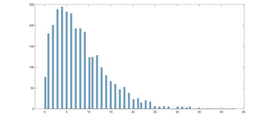
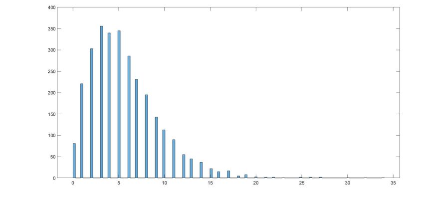
to February 18, 2005. The time series in question, which are plotted in Figure 1, consist of n = 2925
observations and have also been used by Jung et al., (2011). As can be seen from Table 3, each time
series is strongly overdispersed; the sample variance is greater than the sample mean. This is also
verified by the histogram of these series; see Figure 2.
The number of Gibbs iterations was set equal to 5000 with a burn-in period of 5000 updates.
Furthermore, the hyperparameters of the prior distributions for the P -IN SI and N B-IN SI models
are similar to those used in the simulation study. The significance of the parameters was examined
using 95% highest posterior density intervals; see Koop et al. (2007).
5.1.1 Results
The empirical results are presented in Table 4. In particular, it reports the posterior means, standard
deviations, inefficiency factors (IF) and CD statistics for both models and for all data sets. According
to the CD values of this table, the generated sequences of MCMC draws converge for all parameters of
the models. Also, the reported IF values (Table 4) signal a good mixing of the corresponding MCMC
chains, produced by the proposed algorithms.
The figures for the posterior paths, the posterior histograms, and the posterior autocorrelation
functions, for the parameters of both models and for each of the data set in question are given in
an Online Appendix. These figures verify that the posterior paths are stable, while the posterior
autocorrelations decay satisfactory, suggesting that the proposed algorithmic schemes are efficient.
All the parameters in Table 4 are statistically significant. We also observe that the estimated
persistence parameter φ1 is systematically smaller in the P -IN SI model (around 0.7) than in the
N B-IN SI model (around 0.9), whereas the opposite holds for the estimated posterior mean of the
variance σ 2 of the log-volatility equation. From the corresponding posterior histograms (see Online
Appendix), φb1 lies in the stability domain, defined by expression (7). The dispersion parameter in the
N B-IN SI model is the highest in GLT (0.911) and the smallest in EDE (4.89).
According to the reported values of the log of the conditional marginal likelihood (log-CML), the
most preferred model is the N B-IN SI. It has the largest log-CML value for each data set. This is
15also supported by the significance of the τ parameter, which, in any case, is far away from zero (Table
4).
We also considered weighted linear combinations of linear pools (prediction models), which are
evaluated using the log predictive scoring rule (Geweke and Amisano, 2011a). In particular, optimal
weights can be computed in each time t to form a prediction pool for the one-step-ahead forecasting.
Figure 3 shows the evolution of these weights for the last 20 observations of the GLT data set. The
largest weight over the entire out-of sample forecasting period was received by the N B-IN SI model.
The corresponding figures for the EDE and WPP data have been moved to the Online Appendix. In
addition, Table 5 displays the weights for the pool optimized over all of the last 20 observations for
the three financial data sets. The sum of these numbers for each data set is equal to 1. All the weight
is allocated to the N B-IN SI model, with the P -IN SI being excluded from the optimal prediction
pool.
We compared the forecasting performance of the two models, using log predictive scores (LPS) and
RMSFEs. For this out-of-sample forecasting exercise, we calculated density and point forecasts for the
last 20 data points. Table 4 presents the results. Based on the density forecast results, the N B-IN SI
model is the best forecasting model. As far as the point forecasts are concerned, the N B-IN SI model
delivered the lowest RMSFE. In any case, the N B-IN SI model dominates the P -IN SI model, both
in terms of goodness of fit and out-of-sample forecasting ability.
Since N B-IN SI outperforms P -IN SI we focus on the former. Figure 4 shows the real time path of
each time series along b
with the estimated conditional mean λt and the estimated conditional variance,
bt 1 + 1 λ
given by λ b
τb t , obtained from the N B-IN SI model. There is an observed consistent evolution
of these two quantities with the evolution of the original series, where the (conditional) overdispersion
phenomenon is visually highlighted as well.
Given that the proposed specification of this paper attempts to capture the autocorrelation in
the data, it would be appropriate to compare the sample autocorrelations from the data and the
autocorrelations implied by the N B-IN SI model. Hence, we focus on two types of its residuals.
First, the Pearson conditional mean residual (b
ǫt )1≤t≤n (Y -residuals in short) is defined by
b
ǫt =
b q Y t −λ t , 1 ≤ t ≤ n,
b bt )
λt (1+ τ1b λ
bt is the posterior estimate of λt , and λ
where λ b
bt 1 + 1 λ
τb t is the estimated conditional variance of the
model.
Second, we analysed the randomized quantile Y -residuals, defined by Dunn and Smyth (1996)
and used e.g. by Benjamin et al., (2003), Zhu (2011) and Aknouche et al., (2018). The randomized
quantile Y -residuals are especially useful to achieve continuous residuals, when the series is discrete,
as in our case. In the N B-IN SI context, they are given by εbt = Φ−1 (pt ) , where Φ−1 is the inverse
of the standard normal cumulative distribution and pt is a random number uniformly chosen in the
interval h i
F Yt − 1; θb , F Yt ; θb ,
F x; θb being the cumulative function of the negative binomial distribution N B τb, b τb evaluated
λt +bτ
′
at x with parameter θb = φb0 , φb1 , σ
b2 , τb .
The results from the residual analysis are presented in Figure 5 for the GLT data. For example,
in Figure 5 we compare the sample autocorrelations of the observed GLT data (Figure 5a) with those
16of the residuals (Pearson and randomized). We can see that there is significant autocorrelation in the
GLT data series but there is no significant evidence of correlation within the Pearson (Figure 5b) or
randomized Y -residuals (Figure 5c). We repeated the same analysis for the rest of the data sets (EDE
and WPP) and reported the graphical results in the Online Appendix, as the conclusions remained
unchanged.
5.2 Application II: Health data
We also considered, as a second empirical example, the weekly number of a disease caused by Es-
cherichia coli (E.coli) in the state of North Rhine-Westphalia (Germany). The time period of the data
set is from January 2001 to May 2013 with n = 646. The series has been analyzed by various re-
searchers (Doukhan et al., 2006; Silva and Barreto-Souza, 2019) and a graphical view of it is provided
in Figure 6. It is also highly overdispersed, as its sample mean is 20.3344 and its sample variance is
88.7531.
5.2.1 Results
The estimation results are presented in Table 6. No convergence or mixing issues were detected by
inspecting the IF and CD values. The trace plots for the parameters of both models along with
their posterior histograms and autocorrelations are given in the Online Appendix. The estimated φ1
parameters obtained from the two models are high in magnitude; 0.8075 in the P -IN SI model and
0.9012 in the N B-IN SI model. Therefore, there is strong persistence in the evolution of the latent
log-intensities. We also note that the posterior mean of the dispersion parameter is approximately 32
and statistically significant.
Moreover, the N B-IN SI model outperformed the P -IN SI model, both in terms of one-step ahead
(out-of-sample) point and density forecasts (Table 6) for the last 20 observations of the sample. In
Figure 7, the P -IN SI model received the least of the weight over the forecasting period and it is
also excluded from the optimal pool of models; its optimal weight was zero. The conditional marginal
likelihood suggests the N B-IN SI model, as having the best in-sample fit (Table 6).
In Figure 8 we plotted the E.coli series along with the conditional means and variances of the log-
intensities for the N B-IN SI model, which is the dominant one. This figure shows visually that the
data are conditionally overdispersed. This model is also able to pick up most of the serial correlation
present in the E.coli series. This can be seen from the sample autocorrelations of the Y -residuals and
the randomized Y -residuals, given in Figure 9.
6 Conclusions
We proposed an integer-valued stochastic intensity (IN SI) model that conceptually parallels the
stochastic volatility model for real-valued time series. However, like the difference between the
IN GARCH and the GARCH models, the underlying source of dynamics in our model (time-varying
parameter nature of our model) stems from the conditional mean and not the conditional variance,
as in the stochastic volatility framework. The proposed specification is a discrete-valued parameter-
driven model, depending on a latent time-varying intensity parameter, the logarithm of which follows
a drifted first-order autoregression. We focused on a rich class of Poisson mixture distributions that
form a particular IN SI-type model, the mixed Poisson IN SI model.
17Unlike the standard stochastic volatility model, the mixed Poisson IN SI model does not admit a
weak ARMA representation nor a multiplicative error representation but, in spite of that, we easily
studied its probabilistic properties, such as ergodicity, mixing, covariance structure and existence
of higher order moments. The Poisson mixture paradigm has the advantage that its probabilistic
structure allows us to write it as a non-linear stochastic difference equation with i.i.d innovations,
simplifying the study of its probabilistic properties.
Under the Gaussianity assumption for the innovation of the log-intensity equation, we constructed
Markov Chain Monte Carlo algorithms in order to estimate the parameters of the mixed Poisson
IN SI model for two particular conditional distributions; the Poisson and the negative binomial. The
proposed specifications were applied to financial and health data.
It would be interesting to compare the Poisson and negative binomial IN SI models with the
corresponding IN GARCH models, both in terms of model fit and forecasting performance. We leave
that for future research.
18Appendix: Proofs
Proof of Theorem 1. In view of (9), we know that Yt is a causal measurable function of the i.i.d
sequence {(Nt , Zt , et ) , t ∈ Z}. Hence, {Yt , t ∈ Z} is strictly stationary and ergodic. If |φ1 | ≥ 1, then
clearly there does not exist a nonanticipative strictly stationary solution of (1)-(2), like expression
(9).
Proof of Theorem 2. Under the assumptions of Theorem 2 it is clear that the autoregressive process
{log (λt ) , t ∈ Z} is geometrically ergodic and hence is β-mixing (Meyn and Tweedie, 2009). By the
properties of the β-mixing coefficient (e.g. Francq and Zakoian, 2019) it follows that {λt , t ∈ Z} is
also β-mixing. Now, since Yt is a measurable function of λt , then
βY (h) ≤ βλ (h) ,
!
so the result follows, where βY (h) = E sup |P (A/σ {Yt , t ≤ 0}) − P (A)| and so on, with
A∈σ{Yt ,t≥h}
σ {Yt , a ≤ t ≤ b} being the σ-algebra, generated by {Yt , a ≤ t ≤ b}. 5
Proof of Proposition 1. Under (7) and (10)-(12) we have
E (Yt ) = E (E (Nt (Zt λt ) |Zt ))
X∞
φ0
= E exp 1−φ 1
+ φj1 σet−j
j=0
∞
Y
φ0
= E (∆tj ) exp 1−φ1 ,
j=0
which is (13). If, in addition, et ∼ N (0, 1), then using the fact that if X ∼ N (0, 1) it holds
2
E(exp(ϕX)) = exp( ϕ2 ) for any nonnull real constant ϕ, we get
Y
∞ 2
E (Yt ) = exp φ0
1−φ1 exp 12 φj1 σ
j=0
∞
X
= exp φ0
1−φ1 exp σ2
2 φ2j
1
j=0
φ0 σ2
= exp 1−φ1 + 2(1−φ21 )
,
which is (14).
5
Note that {Yt , t ∈ Z} is not a Markov chain but a Hidden Markov chain in the sense of Leroux (1992). So the
result also follows from Proposition 4 of Carrasco and Chen (2002).
19Proof of Proposition 2. Under (7) and (15)-(17) and using (5)-(6) we have
var (Yt ) = E (var (Yt |λt )) + var (E (Yt |λt ))
2
∞
Y ∞
X
= E (∆tj ) exp 1−φ φ0
1
φ0
+ ρ2 + 1 E exp 1−φ 1
+ φj1 σet−j
j=0 j=0
2
∞
Y
φ0
− E (∆tj ) exp 1−φ1
j=0
∞
Y ∞
Y ∞
Y
= E (∆tj ) exp φ0
1−φ1 + ρ2 + 1 E ∆2tj − (E (∆tj ))2 exp 2φ0
1−φ1 ,
j=0 j=0 j=0
which is (18). If, in addition, et ∼ N (0, 1), then using the above normality result we get
∞
Y ∞
Y
σ2
E (∆tj ) = E exp φj1 σet−j = exp 2
(1−φ21 )
j=0 j=0
and
∞
Y ∞
Y 2
2σ 2
E ∆2tj = E exp φj1 σet−j = exp 1−φ21
.
j=0 j=0
Using these results, we get (19).
Proof of Proposition 3. Under (3) and (20)-(21) we have for h > 0
E (Yt Yt−h ) = E [E (Yt Yt−h ) |λt , λt−h ]
X∞ ∞
X
= E exp 1−φ1 +φ0
φj1 σet−j + φ0
1−φ1 + φj1 σet−h−j
j=0 j=0
h−1
Y ∞
Y h i
= exp 2φ0
1−φ1 E (∆tj ) E exp φh1 + 1 φj1 σet−h−j .
j=0 j=0
Hence, (22) follows by calculating E (Yt) E (Yt−h
), using (13).
σ 2 2j
If et ∼ N (0, 1), then E (∆tj ) = exp 2 φ1 and
h−1
Y ∞
Y h−1
Y Y
∞ 2 2
σ 2 2j (φh1 +1) σ
E (∆tj ) E exp φh1 +1 φj1 σet−h−j = exp 2 φ1 exp 2 φ2j
1
j=0 j=0 j=0 j=0
2 2
2h
σ 2 1−φ1 (φh1 +1) σ 1
= exp 2 1−φ21 exp 2 1−φ21
.
Hence, (23) follows by combining the last two expression. Observe that as h → ∞ (under |φ1 | < 1)
γh → 0, which is consistent with asymptotic theory.
Proof of Proposition 4. A) Poisson case: When Yt |λt ∼ P (λt ), it is well known that (e.g. Ferland et
20al., 2006)
r
X s
E (Yts |λt ) = λit .
i
i=0
Hence, under (7) and (24)-(25) we have
E (Yts ) = E (E (Yts |λt ))
Xs X∞
s
= E exp 1−φ iφ0
+i φj1 σet−j
i 1
i=1 j=0
s
X s Y∞
iφ0
= exp 1−φ E ∆itj ,
i 1
i=1 j=0
which is (26).
If, in addition, et ∼ N (0, 1), then using the above normality result we get (27).
ρ−2
B) Negative binomial case: The first four moments of Yt |λt ∼ N B ρ−2 , ρ−2 +λt
are explicitly
given by
E (Yt |λt ) = λt
E Yt2 |λt = λt + 1 + ρ2 λ2t
E Yt3 |λt = λt + 3 1 + ρ2 λ2t + 1 + 3ρ2 + 2ρ4 λ3t
E Yt4 |λt = λt + 7 1 + ρ2 λ2t + 6 + 18ρ2 + 12ρ4 λ3t + 1 + 6ρ2 + 11ρ4 + 6ρ6 λ4t ,
Q
iφ0 ∞
so (28) follows by combining (8), the formula E λit = exp 1−φ j=0 E ∆ i
tj and the fact that
1
Q
i2 σ 2
E (Yts ) = E (E (Yts |λt )) (1 ≤ s ≤ 4). If, in addition, et ∼ N (0, 1), then since ∞ i
j=0 E ∆tj = 2(1−φ2 ) ,
1
we finally get (29).
21References
Ahmad, A., Francq, C. (2016). Poisson QMLE of count time series models. Journal of Time Series
Analysis 37: 291-314.
Aknouche, A. (2017). Periodic autoregressive stochastic volatility. Statistical Inference for
Stochastic Processes 20: 139–177.
Aknouche, A., Bendjeddou, S., Touche, N. (2018). Negative binomial quasi-likelihood inference
for general integer-valued time series models. Journal of Time Series Analysis 39: 192-211.
Aknouche, A., Demmouche, N. (2019). Ergodicity conditions for a double mixed Poisson autore-
gression. Statistics and Probability Letters: 147: 6–11.
Aknouche, A., Francq, C. (2021). Count and duration time series with equal conditional stochastic
and mean orders. Econometric Theory, forthcoming.
Atchadé, Y.F. (2006). An adaptive version for the Metropolis adjusted Langevin algorithm with
a truncated drift. Methodology and Computing in Applied Probability 8: 235–254.
Barra, I., Borowska, A., Koopman, S.J. (2018). Bayesian dynamic modeling of high-frequency
integer price changes. Journal of Financial Econometrics 16: 384–424.
Benjamin, M.A., Rigby, R.A., Stasinopoulos, D.M. (2003). Generalized autoregressive moving
average models. Journal of the American Statistical Association 98: 214–23.
Berg, A., Meyer, R., Yu, J. (2004). Deviance information criterion for comparing stochastic
volatility models. Journal of Business & Economic Statistics 22: 107–120.
Bradlow, E.T., Hardie, B.G.S, Fader, P.S. (2002). Bayesian inference for the negative binomial
distribution via polynomial expansions. Journal of Computational & Graphical Statistics 11: 189–
201.
Carrasco, M., Chen, X. (2002). Mixing and moment properties of various GARCH and stochastic
volatility models. Econometric Theory 18: 17-39.
Chan, J.C.C., Eisenstat, E. (2015). Marginal likelihood estimation with the Cross-Entropy method.
Econometric Reviews, 34: 256–285.
Chan, K.S., Ledholter, J. (1995). Monte Carlo EM Estimation for Time Series Models Involving
Counts. Journal of the American Statistical Association, 90, 242–252.
Chen, C.W.S., So, M., Li, J.C., Sriboonchitta, S. (2016). Autoregressive conditional negative
binomial model applied to over-dispersed time series of counts. Statistical Methodology 31: 73–90.
Chib, S. (2001). Markov chain Monte Carlo methods: computation and inference. In: Handbook
of Econometrics, Volume 5. North Holland, Amsterdam, pp. 3569-3649.
Christou, V., Fokianos, K. (2014). Quasi-likelihood inference for negative binomial time series
models. Journal of Time Series Analysis 35: 55–78.
Christou, V., Fokianos, K. (2015). Estimation and testing linearity for non-linear mixed poisson
autoregressions. Electronic Journal of Statistics 9: 1357—1377.
Cox, D.R. (1981). Statistical analysis of time series: Some recent developments. Scandinavian
22Journal of Statistics 8: 93-115.
Davis, R.A., Dunsmuir, W.T.M., Wang, Y. (1999). Modelling time series of count data. In
Asymptotics, Nonparametrics, and Time Series. CRC Press, New York, pp. 63–114.
Davis, R.A., Dunsmuir, W.T.M., Wang, Y. (2000). On autocorrelation in a Poisson regression
model. Biometrika 87: 491-505.
Davis, R.A., Dunsmuir, W.T.M. (2016). State space models for count time series. In: Handbook
of Discrete-Valued Time Series. Chapman and Hall: CRC Press, pp. 121–144.
Davis, R.A., Holan, S.H., Lund, R., Ravishanker, N. (2016). Handbook of Discrete-Valued Time
Series. Chapman and Hall: CRC Press.
Davis, R.A., Liu, H. (2016). Theory and inference for a class of observation-driven models with
application to time series of counts. Statistica Sinica 26: 1673-1707.
Davis, R.A., Rodriguez-Yam, G. (2005). Estimation for state-space models based on likelihood
approximation. Statistica Sinica 15: 381–406.
Davis, R.A., Wu, R. (2009). A negative binomial model for time series of counts. Biometrika 96:
735–749.
Dean, C., Lawless, J., Willmot, G. (1989). A mixed Poisson-Inverse-Gaussian regression model.
The Canadian Journal of Statistics 17: 171–181.
Doukhan, P., Fokianos, K., Tjøstheim, D. (2012). On weak dependence conditions for Poisson
autoregressions. Statistics and Probability Letters 82: 942–948.
Doukhan, P., Latour, A., Oraichi, D. (2006). A simple integer-valued bilinear time series model.
Advances in Applied Probability 32: 559–578.
Dunn, P.K., Smyth, G.K. (1996). Randomized quantile residuals. Journal of Computational and
Graphical Statistics 5: 236–244.
Efron, B. (1986). Double exponential families and their use in generalized linear Regression.
Journal of the American Statistical Association 81: 709–721.
Engle, R. (2002). New frontiers for ARCH models. Journal of Applied Econometrics 17: 425–446.
Feller, W. (1943). On a general class of “contagious” distributions. Annals of Mathematical
Statistics 14: 389–400.
Ferland, R., Latour, A., Oraichi, D. (2006). Integer-valued GARCH process. Journal of Time
Series Analysis 27: 923-942.
Fokianos, K., Rahbek, A., Tjøstheim, D. (2009). Poisson autoregression. Journal of the American
Statistical Association 140: 1430–1439.
Fokianos, K. (2016). Statistical analysis of count time Series models: A GLM perspective. In:
Handbook of Discrete-Valued Time Series. Chapman and Hall: CRC Press.
Francq, C., Zakoian, J.M. (2019). GARCH Models: Structure, Statistical Inference and Applica-
tions. Wiley.
Freeland, R.K., McCabe, B.P.M. (2004). Forecasting Discrete Valued Low Count Time Series.
International Journal of Forecasting, 20: 427–434.
23You can also read