Testing Hypotheses About Glacial Dynamics Using a Statistical Model of Paleo-Climate

Testing Hypotheses About Glacial Dynamics Using
a Statistical Model of Paleo-Climate
Robert Kaufmann (  kaufmann@bu.edu )
 Boston University https://orcid.org/0000-0002-5670-7027
Felix Pretis
 University of Victoria

Research Article

Keywords: Glacial cycles, linear, nonlinearity, termination, Mid-Brunhes event

Posted Date: April 27th, 2021

DOI: https://doi.org/10.21203/rs.3.rs-459880/v1

License:   This work is licensed under a Creative Commons Attribution 4.0 International License.
Read Full License

1

1

2 Testing Hypotheses About Glacial Dynamics Using a Statistical Model of Paleo-Climate

3 Enter authors here: Robert K. Kaufmann1, Felix Pretis2
 1
4 Department of Earth and Environment, Boston University, Boston, Massachusetts, USA, 02215
5 OCRID ResearcherID:I-4962-2017
6
 2
7 Department of Economics, University of Victoria, Victoria, BC, Canada; and Nuffield College,
8 University of Oxford, Oxford, UK ORCID 0000-0003-1435-9295
9

10 Corresponding author: Robert K. Kaufmann (Kaufmann@bu.edu)

11 Key Words: Glacial cycles, linear, nonlinearity, termination, Mid-Brunhes event
12

2

13

14 Abstract
15 We test hypotheses about glacial dynamics by evaluating the ability of a linear statistical model to

16 simulate climate during the previous ~800,000 years. During this period, the linear model

17 simulates the timing and magnitude of glacial cycles, including the saw-tooth pattern in which ice

18 accumulates gradually and ablates rapidly, without falsely simulating an interglacial after each

19 peak in obliquity. Conversely, the linear model fails to simulate experimental observations that are

20 created by a nonlinear data generating process. Together, these (in)abilities suggest that

21 nonlinearities, threshold effects, bifurcations, and/or phase-specific governing equations do not

22 play a critical role in glacial cycles during the late Pleistocene. Furthermore, the model’s accuracy

23 throughout the sample period suggests that changes in orbital geometry create the Mid-Brunhes

24 event.

25

3

26

27 1 Introduction
28 When considered over the last eight-hundred thousand years, climate shows highly persistent
29 patterns. Most notable are glacial cycles. During glaciations, temperature, greenhouse gas
30 concentrations, and sea level remain below their sample mean for extended periods; during these
31 same periods, land and sea ice remain above their sample means (Kaufmann and Juselius, 2013).
32 These positions are reversed for extended periods known as interglacials. These persistent
33 movements and complex climate dynamics create difficulties for statistical analyses of climate
34 data. Using ordinary least squares to analyze time series that show persistent movements tends to
35 greatly inflate findings of a statistically meaningful relations among time series when none are
36 present (Yule, 1929; Engle and Granger, 1987).
37 Difficulties posed by highly persistent movements and complex dynamics are alleviated using
38 vector-autoregression, cointegration, and equilibrium correction (Kaufmann and Juselius, 2013).
39 Using these methods, Kaufmann and Juselius (2013), herein KJ2013, estimate a linear statistical
40 model of climate from a sample that includes observations from the previous 391 thousand years.
41 The model, termed a cointegration vector autoregression (CVAR), specifies linear relations
42 between four exogenous variables for orbital geometry; eccentricity (Ecc), obliquity (Obl),
43 precession (Prec), and summer time insolation at 65o south SunSum (Supplementary Note 1) and
44 ten endogenous climate variables; Antarctic land (Temp) and sea surface temperature (SST), carbon
45 dioxide (CO2) and methane (CH4) concentrations, land (Ice) and sea ice (Na), sea level (Level),
46 iron dust (Fe), and non sea-salt sulfate (SO4) and calcium (Ca), which are chosen to proxy physical
47 relations thought to drive glacial cycles (Kaufmann and Juselius, 2013, Supplementary Note II).
48 The CVAR model explicitly represents linear long-run equilibrium relations between orbital
49 geometry and climate, which are given by ten cointegrating relations, and climate dynamics, which
50 are given by constant rates at which the climate system adjusts towards the equilibrium given by
51 the long-run (cointegrating) relations. A similar approach is applied to a subset of climate variables
52 (Davidson et al., 2016).
53 As described in Kaufmann and Juselius (2013; 2016) as well as Kaufmann and Pretis (2021),
54 these statistical relations validate some basic hypotheses about the mechanisms that are postulated
55 to drive glacial cycles (e.g. carbon dioxide affects temperature via radiative forcing), reproduce

4

56 the main features of glacial cycles (e.g. the timing, magnitude, and saw-tooth pattern of changes
57 in land ice volume), and separate observed interglacial periods from skipped/missing beats (e.g.
58 Huybers, 2012), which are peaks in insolation (e.g. obliquity) that do not generate deglaciations
59 and thus interglacials. Over the last million years, twelve of the twenty-five peaks in obliquity are
60 not associated with deglaciations (Tzedakis et al., 2017).
61 To date, efforts to explain missing beats in particular, and glacial cycles in general, focus on
62 nonlinear relations (e.g. Tziperman et al., 2006), threshold effects (e.g. Paillard, 1998; 2001,
63 Ganopolski et al., 2016), bifurcations (e.g. Ashwin and Ditlevsen, 2015) and/or phase-specific
64 governing equations (e.g. Tzedakis et al., 2017). Some of these dynamics are embodied in several
65 models that account for many features of the glacial cycle (e.g. Parrenin and Paillard, 2012;
66 Paillard and Parennin, 2004). Based on these successes, there is a consensus that nonlinearities,
67 threshold effects, bifurcations, and/or phase specific governing equations play a critical role in
68 glacial cycles in general and terminations in particular, as summarized by a recent review
69 “Terminations clearly represent a strongly nonlinear response to regional changes in the
70 seasonality of solar radiation (Past interglacials Working Group of Pages, 2016).”
71 Here, we explore this consensus using a linear CVAR model reported by KJ2013. Specifically,
72 is the success of previous models based on their inclusion of nonlinearities, threshold effects,
73 bifurcations, or phase-specific governing equations, etc? To test this hypothesis, we evaluate
74 whether a model that omits nonlinearities, threshold effects, bifurcations, and/or phase-specific
75 governing equations can accurately simulate glacial cycles. To answer, we test whether a statistical
76 model that specifies linear relations among orbital geometry and climate variables can simulate
77 glacial cycles accurately. If a linear model can simulate glacial cycles accurately, the logic of
78 Occam’s razor implies that nonlinearities, threshold effects, bifurcations, and/or phase-specific
79 governing equations are complexities that do not play a critical in glacial cycles beyond linear
80 relations. Conversely these complexities likely play an important role if a simple linear model
81 without nonlinearities, threshold effects, bifurcations, and/or phase-specific governing equations
82 cannot accurately simulate glacial cycles. Specifically, we formulate and test three hypotheses.
83 1. To establish the capabilities of the CVAR model, we asses the degree to which the linear
84 specification of the CVAR model is able to simulate non-linear relations among
85 experimental data that are simulated by non-linear Van der Pol Oscillators. We postulate
86 that a linear CVAR model will not be able to simulate non-linear relations among the

5

87 experimental data. Consistent with this hypothesis, the linear CVAR model is not able to
88 simulate the non-linear relations among an exogenous forcing, which mimics orbital
89 geometry, and two endogenous variables which mimic components of climate that react
90 quickly (temperature) and slowly (ice volume) to changes in orbital geometry.
91 2. We assess the ability of the linear CVAR to simulate (out-of-sample and in-sample) ten
92 endogenous variables that represent important components of the observed paleo-climate
93 record based on four variables that represent orbital geometry. We postulate that the linear
94 CVAR model will fail to simulate glacial cycles accurately if nonlinearities, threshold
95 effects, bifurcations, and/or phase-specific governing equations play an important role in
96 the timing and magnitude of glacial cycles. But if their role is small relative to linear
97 relations, we postulate that the linear CVAR model will simulate glacial cycles accurately,
98 both during the in-sample period used to estimate the model (391 Kyr BP – present) and
99 an out-of-sample period (792 Kyr BP – 392 Kyr BP). Compared to its poor performance
100 with the nonlinear experimental data generated by Van der Pol oscillators, the linear CVAR
101 model is able to account for a much larger portion of the variation in climate variables
102 during both the in- and out-of-sample periods. Furthermore, the model errors are
103 distributed randomly between interglacials and the other phases of the glacial cycle. This
104 performance suggests that nonlinearities, threshold effects, bifurcations, or changes in
105 governing equations do not play a critical role in the timing or magnitude of glacial cycles.
106 3. We assess the ability of the linear CVAR model to simulate glacial cycles before and after
107 the Mid-Brunhes event (MBE), in which CO2 concentrations rise, the amplitude
108 interglacials increase, and interglacials are cooler but longer starting about 430 thousand
109 years before the present (EPICA, et al., 2004; Luthi et al., 2008; Hoenisch et al., 2009,
110 Jansen et al., 1986). If changes in orbital geometry play an important role in the MBE, there
111 will be little change in the ability of the linear CVAR model to simulate glacial cycles
112 before and after the MBE because the CVAR model specifies the same relations between
113 orbital geometry and climate before and after the MBE. But if changes in long- and short
114 run relations between orbital geometry and climate variables create the changes in glacial
115 cycles that are associated with the MBE, the CVAR’s ability to simulate glacial cycles
116 before the MBE will be diminished relative to the period after the MBE. This is because
117 the linear CVAR is estimated from observations after the MBE and uses that these long-

6

118 and short-run relations to simulate the period before the MBE. Results indicate that model
119 performance does not change around the MBE, which suggests that the MBE is driven by
120 changes in orbital geometry.
121 These results and the methods used to obtain them are described in five sections. Section 2
122 describes the data and methods used to generate and analyze the simulations. The results are
123 reported in section 3, discussed in section 4, and section 5 concludes.

124 Methods
125 2.1. The CVAR Model Specifies Linear Relations Among Variables
126 The equations used by the linear CVAR model to estimate long- and short-run relations between
127 orbital geometry and climate are given by:
128 ∆ $ = ' ∆ $ + * ∆ $+* + Γ* ∆ $+* + Γ- ∆ $+- + Π $+*
 0
 + $ (1)
129 in which $ is a 10 × 1 vector that includes the ten endogenous variables; Temp, CO2, CH4, Ice,
130 Fe, Na, Ca, SO, Level, and SST (Table 1); w is a 4 × 1 vector that includes the four exogenous
131 variables for orbtial geometry Ecc, Prec, Obl, and Sunsum, 0 = [ $0 , $0 , 1], Γ* (10 ×
132 10 ), ' (10 × 4 ), * (10 × 4 ), are matrices of short-run coefficients; Π is a 10 × 15 matrix of
133 long-run coefficients, ∆ is the first difference operator (∆ $ = $ − $+* ), and = is an error term
134 with mean value zero and variance Ω that is normally, independently, and identicially distributed.
135 The condition that the conditional process ( $ | $ ) is nonstationary is formulated as a reduced
136 rank hypothesis on the matrix Π:
137 Π = 0 (2)
138 in which is a 10 × matrix of coefficients, which describe a constant rate at which the ten
139 climate variables (or I and T in the experimental data set) adjust towards the equilibrium that is
140 given by orbital geomtery (or F in the experimental data set); is the number of cointegration
141 relations given by the reduced rank of the Π matrix and is a × 15 matrix of cointegration
142 coefficients that define the r stationary deviations from long-run equilibrium relations, the so
143 called cointegration relations, 0 $ . Using maximum likelihood techniques, KJ2013 estimate the
144 and matrices (Supplementary Tables 2 and 3) KJ2013 from a partial system (Johansen 1992,
145 Harbo et al., 1998, Juselius 2006) in which orbital variables are weakly exogenous (i.e. changes in
146 climate do not affect orbital geometry). To identify the equations and generate standard errors for
147 the statistical parameters, KJ2013 impose 26 overidentifying restrictions on the matrix. No

7

148 restrictions are imposed on the CVAR model that is estimated from the experimental data to
149 maximize its ability to simulate I and/or T (hypothesis 1).
150 Despite its complexity, the CVAR model is linear in parameters. Equilibrium relations, as
151 represented by the cointegrating relations 0 $ specify linear relations (in levels) among variables,
152 and changes in variables are modelled as linear functions of disequilibrium. To illustrate, the tenth
153 cointegrating relation in KJ2013 (Supplementary Table 2) represents a linear long-run equilibrium
154 relation between Ice and orbital geometry which can be used to represent the equilibrium level of
155 Ice that is implied by orbital geometry as follows:
156 Icet = -0.755*Ecct + 4.459*Oblt + 2.881*SunSumt (3)
157 Statistically significant coefficients associated with Obl and SunSum indicate that obliquity has
158 information about Ice that is not contained in SunSum and vice-versa, despite their strong
159 correlation. Similarly, there are strong correlations among the four variables for orbital geometry,
160 but statistically significant coefficients indicate that no combination of three contains all of the
161 information in the fourth.
162 System dynamics are represented by adjustment towards equilibrium ( ), which is constant
163 (over all phases of the glacial cycle) and is a linear function of disequilibrium in the level of the
164 variables in the previous time period. For Ice, 3.7 percent of the disequilibrium between the
165 previous period’s equilibrium value (as implied by the tenth cointegrating relation equation (3))
166 and the previous period’s value is eliminated each period:
167 ∆ $ = −0.037 × I $+* − (−0.755 ∗ $+* + 4.459 ∗ $+* + 2.881 ∗ $+* )S (4)
168 A constant rate of adjustment 3.7 percent implies a constant adjustment time, which does not
169 represent the nonlinearities of ice flow and mass balance for an ice sheet (Roe, 2006). Roe (2006)
170 argues that these nonlinearities are critical “the nonlinearities of ice flow and mass balance
171 preclude the application of a single adjustment time scale to an ice sheet.” This contention is test
172 by hypothesis 2. If nonlinearities associated with ice sheet and other aspects of the climate are
173 important, their omission will prevent the linear CVAR model from simulating ice volume
174 accurately. Conversely if the nonlinearities of ice flow and mass balance for an ice sheet do not
175 play a critical role in glacial cycles, the linear CVAR model may accurately simulate ice volume
176 in particular, and glacial cycles in general.
177 Equations 1 and 2 specify many parameters, but the statistical model is not ‘overfit.’ In KJ2013,
178 each of the ten dependent variables in $ has 390 observations. Each equation has 357 degrees of

8

179 freedom because the Π, Γ, ' and * matrices specify 33 coefficients for each of the ten equations.
180 These 33 coefficients correspond to the 15 columns in the Π matrix (including a constant), the 10
181 columns in the Γ matrix, and the four columns in the Ao and A1 matrices. Of these 33 coefficients,
182 many are not statistically different from zero (Supplemental Table 4). As a result, the ten equations
183 contain between 7 and 16 variables per equation, which is consistent with the range suggested by
184 Maasch and Saltzman (1990). Thus, the ~357 degrees of freedom alleviates any concern the the
185 equations are ‘overfit.’
186 Finally, the correlation among the ten endogenous climate variables has little effect on the
187 model’s ability to simulate glacial cycles. The model is driven by the four exogenous variables for
188 orbital geometry; the model has no information about any of the climate variables beyond the
189 values used to initialize the model. Under these conditions, the statistical relations in the linear
190 CVAR model translate changes in orbital geometry into changes in climate but do not contain
191 information about climate beyond that contained in the variables for orbital geometry.
192 To make all data amenable to a statistical analysis, KJ2013 converts observations from the
193 proxy record to a common time scale (EDC3) using conversions from Parrenin et al., (2007) and
194 Ruddiman and Raymo (2003). Unevenly spaced observations are interpolated (linearly) to
195 generate a data set in which each series has a time step of 1 kyr, which has relatively little effect
196 on results (Miller, 2019). To eliminate the effects of inverting matrices with elements that differ
197 greatly in size (due to different units of measurement), each of the fourteen time series is
198 standardized as follows:
199 = = ( $ − U)/W ( ), = 1, … ,391 (5)
200 in which $ is the value (in original units), y is the mean value over the 391 Kyr in-sample period,
201 and ( ) is the variance over the in-sample period. Equation (5) also is used to normalize the
202 1000 observations in the experimental data generated by the Van der Pol oscillators (Section 2.2).
203 We recognize that nonstationary time series do not have a constant mean or variance, rather the
204 sample mean and variances are used in a linear transformation to harmonize the values of the time
205 series.
206 2.2 Generating Experimental Data with Non-Linear Relations
207 To test whether the linear CVAR model can simulate non-linear processes, we use the CVAR
208 methodology to estimate the relation among experimental data that are generated by non-linear
209 van der Pol oscillators (Crucifix, 2013). Using the parameters specified by Crucifix (2013), van-

9

210 der-Pol oscillators create experimental data that mimic paleo-climate data. Specifically, a
211 sinusoidal forcing F, which mimics changes in orbital geometry, is perturbed with white noise to
212 simulate a variable ‘T’ that responds rapidly to F (such as temperature), while variable ‘I’ mimics
213 a variable that responds gradually (such as ice). This process is used to create 1,000 observations
214 in discrete time for each variable (Figure 1(a) & (b)). We use the first 500 observations to estimate
215 the CVAR model. The remaining 500 observations constitute an out-of-sample period.
216 2.3 Simulating Experimental Data or Observed Climate Variables using a Linear CVAR Model
217 To assess hypothesis 1-3, we simulate the linear CVAR model of climate over a ~ 800 kyr
218 sample period, which includes a 391 Kyr BP – present in-sample period that used to estimate the
219 model (Kaufmann and Juselius, 2013) and a 792 Kyr BP – 392 Kyr BP out-of-sample period. To
220 simulate climate during the in- and out-of-sample periods, the ten endogenous variables x (or two
221 experimental data simulated by the Van der Pol Oscillators) are expressed as a function of the
222 exogenous variables for orbital geometry (or the exogenous variable used to drive the Van der Pol
223 Osciallators) and shocks to the climate system ( ) by inverting Equation (1) into the moving
224 average form:
225 $ = ∑$=^* $ + ∗ ( ) $ + ` $ + `∗ ( )Δ $ (5)
226 In which = b (1 − Γ* )+* b ; b is a 10 × (10 − ) matrix orthogonal to describing the
227 stochastic trends and b is a 10 × (10 − ) matrix orthogonal to determining how the stochastic
228 trends load into the climate variables; L is the lag operator (for example, $ = $+* ); ∗ ( ) and
229 `∗ ( ) are stationary lag polynomials; ` is 10 × 4; and the matrices are functions of the
230 parameters ( ', *, Γ*, , ). Based on the ten cointergating relations reported by KJ2013 r = 10,
231 then C = 0, the in- and out-of-sample simulations are based on model (2) subject to (3) by setting
232 $ = 0 which implies that the simulated variables, c$ , are calculated from the exogenous drivers,
233 ` $ , ( ' ∆ $ ), the dynamics attached to them, `∗ ( )∆ $+* , ( * ∆ $+* ), and the internal climate
234 dynamics ∗ ( ) $ (Γ* Δ c$+* , 0defg ).
235 The out-of-sample simulation is initialized using observed values for Temp, SST, and Ice, which
236 are available starting 800 kyr BP. The time series for CO2 CH4, Fe, Na, SO4, Ca, and Level have
237 more recent start dates (Table 1). For these variables, the model is initialized with values that
238 correspond to their sample mean. We use these values to ‘spin up’ the model so that the simulated
239 values converge towards observed values and looses sensitvity to initial conditions. Following this
240 10 Kyr ‘spin-up,’ which is shorter than other climate models (e.g. Parrenin and Paillard, 2012), the

10

241 model is run continuously through the present. Because the simulation starts the out-of-sample
242 period, this ordering adds rigor. That is, error in the out-of-sample simulation are passed to the
243 start of the in-sample simulation.
244 2.3 Assessing model performance
245 There are many ways to assess model performance. Previous analyses use spectral analyses,
246 which evaluate the degree to which the power spectrum of the observed and simulated data match
247 (e.g. Ditlevsen et al., 2020). These efforts focus on the 100 Kyr frequency. But this emphasis is
248 made difficult by the paucity of observations; by definition, there are only eight possible peaks at
249 the 100 Kyr frquency in the 800 Kyr record that are recorded in cores recovered from the Antarctic
250 ice.
251 Instead, we focus on the model’s ability to simulate each of the 792 observations for each of
252 the 1Kyr time steps. First, we quantify the model’s skill in replicating glacial cycles based on the
 ∑k
 lmg(ie +ice )
 j
253 size of errors as measured by root mean square error (RMSE) h n
 in which c$ is the value

254 for variable at time t simulated by the model, $ is the observed value for the proxy, and T is the
255 number of observations. The fraction of variation that is explained by the linear CVAR model is
256 quantified by the adjusted r2, which is estimated from the following regression:
257 $ = + c$ + $ (6)
258 in which and are regression coefficient estimated using ordinary least squares and is the
259 regression residual. For ice, the r2 quantifies the fraction of variation that is observed in the 792
260 observations that is explained by the 792 values for Ice that are simulated by the linear CVAR
261 model.
262 For each variable x, we use the simulation errors ( $ = $ − c$ ) to identify periods when
263 model accuracy changes in a statistically significant fashion, such as stage 111. We identify these
264 periods with an indicator saturation technique [R-package gets Pretis et al., 2018; Castle et al.,
265 2015]. This approach is used to assess the time-varying performance of climate models (Pretis et
266 al., 2015), the forecast accuracy of economic predictions (Ericsson 2017), and the presence of
267 volcanic eruptions in temperature reconstructions in both simulated climate data (Pretis et al.,
268 2016) and proxy-reconstructions (Schneider et al., 2017).

 1
 Stage 11 is a well-known mismatch between orbital geometry and an interglacial period (e.g. Imbrie et al., (1993))
 that occurs between 424,000 and 374,000 years ago.

11

269 This indicator saturation technique can identify the date(s) when the value for each of the ten
270 variables simulated by the linear CVAR model c deviates significantly from x (i.e. simulation
271 errors are statistically different from zero) for a single time-step (outlier). Persisting errors are
272 values of c that deviate significantly from x for two or more consecutive time-steps
273 (Supplementary Note III). Outliers and persisting errors are evaluated for every possible time step.
274 We retain only those outliers or persisting errors that exceed a pα = 0.001 threshold. This threshold
275 implies that random chance will cause the technique to identify one outlier (or persisting error) per
276 1,000 observations. This tightly controls the false-positive rate of detected periods of model
277 failure.
278 If model performance does not change in a systematic fashion through phases of the glacial
279 cycle or over time, we expect outliers and persisting errors to occur randomly throughout the
280 sample. For each of the ten endogenous variables (and as a group), we compare the distribution of
281 outliers and persisting errors between interglacial and non-interglacial periods, as defined by
282 Tzedakis et al., (2012) and between the in-sample and out-of-sample periods. We test whether the
283 timing of outliers and persisting errors across the sample period is different from a uniform random
284 distribution (expected under the null-hypothesis of equal performance) using a Pearson chi-square
285 test (P), which is calculated as follows:
 j
 Iuv +wv S
286 = ∑xy^* wv
 (7)

287 in which n is two periods (interglacial j = 1; non-interglacial j = 2; or in-sample j = 1; out-of-
288 sample j = 2), Oj is the number of outliers or persisting errors that are identified in period j, and Ej
289 is the number of outliers or persisting errors that are expected in period j.
290 The number of outliers or persisting errors expected in period j (Ej) is calculated based on the
291 null hypothesis that outliers or persisting errors are distributed uniformly between periods. This
292 null implies that the expected number outliers or persisting errors ( y ) can be calculated as:
 z{v
293 y = ∑|
 × ∑xy^* y (8)
 l z{vl

294 in which Yr is the number of thousand-year time steps in period j for which simulated and observed
295 values are available and n is the number of thousand year time steps in the simulation period. P is
296 evaluated against a - distribution with n-1 degrees of freedom. If the test rejects the null
297 hypothesis that outliers or persisting errors are distributed randomly between interglacial and non-
298 interglacial phases of the cycle (i.e. some phases are simulated more/less accurately than others),

12

299 the more accurate phase is identified by the numerator of Equation (7) ( y − y ). A negative value
300 for interglacial periods (( * − * ) < 0) would indicate that the number of outliers or persisting
301 errors detected during the interglacial phase of glacial cycles is less than expected by a uniform
302 random distribution and hence the interglacial phase of glacial cycles is simulated more accurately
303 than other phases of the glacial cycle.
304 2.4 Testing Hypothesis 3: The Mid-Brunhes event (MBE) represents a change in the dynamics
305 that drive glacial cycles
306 The start of the in-sample period used to estimate KJ2013 falls close to the Mid-Brunhes event,
307 which occurs about 430 thousand years before present (Jansen et al., 1986). To test hypothesis 3,
308 we compare the model performance before and after the MBE. Specifically, we compare the adjust
309 r2, RMSE, and the distribution of outliers and persisting errors between the in- and out-of-sample
310 periods. If these metrics indicate that the model performs equally well, this would be inconsistent
311 with the hypothesis that the MBE represents a change in the long- and/or short-run relations in the
312 climate system because these relations are held constant by the climate model. Instead, results that
313 indicate model performance does not change would be consistent with the hypothesis that changes
314 in orbital geometry drive the changes in glacial cycles that are associated with the MBE.
315

316 3 Results & Discussion
317 3.1 The linear CVAR model is not able to simulate non-linear relations
318 Using the linear CVAR model to estimate the non-linear relations among F, I, and T in the
319 experimental data generates coefficients that are statistically different from zero (Supplementary
320 Tables 5 and 6). But visual inspection of Figure 1(a-b) indicates that the resultant CVAR model is
321 not able to simulate T or I during the in- or out-of-sample periods in a statistically meaningful
322 fashion. Specifically, the simulated values for T and I account for a small portion of the variation
323 in the T and I as measured by the r2 for equation (6) during any of the sample periods (Table 2).
324 This poor performance implies that imposing a linear specification on the long- and short-run
325 relations between the exogenous forcing (F) and the endogenous variables (I or T) cannot capture
326 the non-linear relation among these variables that is created by the nonlinear data generating
327 process. This inability is not offset by the lagged short-run effects represented by coefficients in
328 the A or Γ matrices, which is set to two lags, which is consistent with the lag length used in KJ2013.
329 Together, these failures indicate that the linear CVAR model cannot capture non-linear relations.

13

330 The inability of the linear CVAR model to capture nonlinear relations among the experimental
331 data (Figure 1(a-b)) suggests that the linear CVAR model can be used to test whether nonlinear
332 processes, threshold effects, bifurcations, or changes in governing equations play an important role
333 in glacial cycles. If nonlinear processes, threshold effects, bifurcations, or changes in governing
334 equations play an important role in glacial cycles, the inability of the CVAR model to quantify
335 nonlinear relations will prevent the CVAR from simulating glacial cycles accurately, as indicated
336 by Figure 1 and the values for r2 in Table 2. Conversely, if nonlinear processes, threshold effects,
337 bifurcations, and/or governing equations that vary by phase of the glacial cycle play a lesser role,
338 and linear relations are largely responsible for the timing and magnitude of glacial cycles, a
339 properly specified linear model, such as a CVAR, will be able to simulate glacial cycles more
340 accurately than indicated in Figure 1 and Table 2.
341 3.2 Hypothesis 1(b) Nonlinearities, threshold effects, and/or phase-specific governing equations
342 play an important role in the timing and magnitude of glacial cycles
343 For both the in- and out-of-sample periods, Figure 2 suggests that KJ2013 generally captures
344 the timing and magnitude of persistent changes in climate that are described by glacial cycles.
345 These cycles often are summarized by changes in land ice volume. Simulated values for Ice follow
346 the saw-tooth pattern in which ice volume builds slowly but ablates rapidly (Figure 2d).
347 Furthermore, the CVAR model generally simulates the timing and magnitude of changes in ice
348 volume accurately (other than stage 11) without falsely simulating an integlacial after each peak
349 in obliquity (i.e. missing beats). Consistent with these abilities, the r2 values in Table 2 indicate
350 that the linear CVAR model is able to account for about 60 percent of the variation in Ice and Temp
351 dring the in-sample and out-of-sample periods (when stage 11 is excluded). This is considerably
352 larger than the ~20 percent of the in-sample variation in temperature that is captured by a statistical
353 model by Wunsch (2004). Similarly, the linear CVAR model is able to account for 20 – 60 percent
354 of the variation in the eight other variables for climate, both in- and out-of-sample (Table 2). All
355 of these values are larger than the portion of variation (0.04 – 0.16) in the nonlinear experimental
356 data that is simulated by the linear CVAR.
357 The visual suggestion in Figure 2 that the CVAR model is able to simulate all phases of glacial
358 cycles with a modicum of accuracy is confirmed by tests that fail to reject the null hypothesis that
359 outliers and persisting errors for Ice (and the other nine endogenous variables) are distributed
360 randomly between interglacials and all other phases of glacial cycles (Table 3). This result suggests

14

361 that nonlinearties, threshold effects, bifurcations, and/or changes in governing equations are not
362 needed to simulate various phases of the glacial cycle.
363 The ability of the linear CVAR model to simulate seemingly non-linear changes in ice volume
364 and the other nine variables likely stems from two sources. When a variable is far from equilibrium,
365 the constant rate of adjustment ( ) in the linear model moves the variable towards equilibrium by
366 a larger amount than when that variable is closer to equilibrium. Second, the model is conditioned
367 on orbital geometry, which changes nonlinearly over time. But the VAR model specifies these
368 nonlinear changes with a linear relation between orbital geometry and climate variables. As such,
369 non-linear changes in orbital geometry have a linear relation with the ten endogenous variables for
370 climate that are simulated by the linear CVAR model.
371 The ability of the linear CVAR model to simulate all phases of the glacial cycles and the in-
372 and out-of-sample periods (see below) is inconsistent with the hypothesis that nonlinearties,
373 threshold effects, bifurcations, and/or phase specific governing equations play a critical role in
374 glacial cycles. Instead, results suggest that non-linear relations, thresholds, bifurcations, and/or
375 changes in governing equations do not play a critical role in glacial cycles since the mid Pleistocene
376 transition (MPT). Nonetheless, our results do not reject the presence of non-linear relations,
377 thresholds, bifurcations, or changes in governing equations. We do not argue that linear relations
378 govern ice flow and the mass balance; these processes clearly have a nonlinear component (e.g.
379 Roe and Lindzen, 2001). But the linear CVAR model does not need to represent the nonlinear
380 components of ice flow and mass balance to simulate glacial cycles accurately. Instead, the timing
381 and magnitude of glacial cycles can be described by linear long- and short-run relations between
382 orbital geometry and the climate system. Interpreting these results through the filter of Occams
383 razor suggests that the current emphasis non-linear relations, thresholds, bifurcations, or changes
384 in governing equations is misplaced; important drivers of glacial cycles can be understood using
385 linear models.
386 Furthermore, the ability of the CVAR model to simulate climate during the out-of-sample
387 period is inconsistent one of the extreme explanations that is listed by Tziperman et al., (2006)
388 “glacial cycles would exist even in the absence of the insolation changes.” If glacial cycles exist
389 independently of changes in orbital geometry, a statistical model that is conditioned only on orbital
390 geometry and spun up with no memory of previous cycles would not be able to simulate glacial
391 cycles accurately during the initial out-of-sample period. Furthermore, if orbital geometry is held

15

392 constant, the ten endogenous variables in the CVAR model come to an equilibrium and do not
393 change thereafter, which is consistent with physically-based models (e.g. Ganopolski and Brovkin,
394 2017).
395 Finally, the model’s ability to simulate glacial cycles during the out-of-sample period is
396 inconsistent with speculation that the CVAR model’s ability to reproduce the ten endogenous
397 variables during the in-sample period simply reflects the model’s ability to reproduce the data used
398 to estimate the coefficients. Instead, the ability of the model to simulate climate during the out-of-
399 sample period suggests that the regression coefficients in the Π, Γ, ' and * matrices capture long-
400 and short-run relations among orbital geometry and the ten endogenous variables that govern the
401 climate system for the 400 kyr before the sample period used to estimate the model.
402 3.3 Testing hypothesis 3: The Mid-Brunhes event (MBE) represents a change in the dynamics that
403 drive glacial cycles
404 The linear CVAR model is able to simulate glacial cycles during the in- and out-of-sample
405 periods as indicated by root mean square error and r2 (Table 2). As expected, the RMSE for the
406 out-of-sample period generally is larger than the RMSE for the in-sample period. Consistent with
407 this expectation, the r2 is larger for the in-sample period. But much of these differences are
408 associated with MIS 11 (424 – 375 Kyr BP), most of which occurs during the out-of-sample period
409 (Table 2). If we eliminate MIS 11 from the out-of-sample period, the RMSE and r2 of the in- and
410 out-of-sample periods are similar (Table 2).
411 The small change in accuracy between the in- and out-of-sample periods is confirmed by the
412 distribution of outliers and persisting errors (Figure 3). Tests indicate that we cannot reject the null
413 hypothesis that outliers are distributed randomly between the in- and out-of-sample periods (Table
414 3). A test statistic χ- (1) = 0.09 fails to reject (p > 0.76) the null hypothesis that as a group, outliers
415 for the ten endogenous variables are distributed randomly between the in- and out-of-sample
416 periods. Conversely, a test statistic χ- (1) = 52.5 rejects (p < 0.001) the null hypothesis that as a
417 group, persisting errors for the ten endogenous climate variables are distributed randomly between
418 the in- and out-of-sample periods. But this rejection may be somewhat misleading. The out-of-
419 sample simulation for CH4 and Ice is more accurate than the in-sample simulation.
420 The relatively small changes in model performance for the in- and out-of-sample periods
421 suggests that the MBE does not change the ability of the linear CVAR model to simulate glacial
422 cycles. Compared to the in-sample period used to estimate KJ2013, the pre-MBE out-of-sample

16

423 period has; (1) lower concentrations of CO2, (2) glacial cycles with a smaller amplitude, and (3)
424 cooler but longer interglacial periods (EPICA, et al., 2004; Luthi et al., 2008; Hoenisch et al.,
425 2009). These three changes can be caused by one or both of two possible mechanisms. Glacial
426 cycles may change at the MBE due to changes in the orbital geometry that drive glacial cycles,
427 “through a set of internal mechanisms, insolation alone induces a systematic difference between
428 the interglacials before and after the 430 kyr ago (Yin, 2013).” Alternatively, glacial cycles may
429 change at the MBE due to changes in the endogenous dynamics that link orbital geometry to the
430 climate system, “astronomical forcing alone cannot explain the difference in interglacial intensity
431 before and after the MBE (Tzedakis et al., 2009).”
432 The CVAR model uses the linear long- and short-run relation estimated from the previous 391
433 kyr sample period to simulate the climate system before the MBE. The lack of a meaningful change
434 in accuracy suggests that the same physical relations generate glacial cycles before and after the
435 MBE. As such, our results are inconsistent with the hypothesis that “astronomical forcing alone
436 cannot explain the difference in interglacial intensity before and after the MBE (Tzedakis et al.,
437 2009).” Instead, the lack of a meaningful change in accuracy suggests that orbital geometry alone
438 can account for the three changes in glacial cycles before and after the MBE.
439

440 4 Conclusion
441 Using only linear relations between orbital geometry and ten endogenous variables, the linear
442 CVAR model is able to accurately simulate the evolution of climate during ~ 400 kyr in- and out-
443 of-sample periods during all phases of the glacial cycles. This ability suggests that non-linearities,
444 thresholds, bifurcations, and/or changes in governing equations do not play a critical role in glacial
445 cycles. Furthermore, there is little evidence that the MBE changes the underlying relations between
446 orbital geometry and the climate system.
447 Nonetheless, the accuracy of the CVAR model declines in a statistically significant manner
448 during MIS stage 11 and Termination V, which is consistent with arguments that the ‘stage 11
449 paradox’ is a mismatch between orbital geometry and climate (Imbrie et al., 1993). To investigate
450 the causes for the ‘stage 11 problem’ we will analyze the statistical orderings of simulation errors
451 to identify the equations that initiate the model’s poor performance. In other words, the statistical
452 ordering of simulation errors may allow the model to identify what is unique about MIS 11 (and
453 termination V).

17

454 The accuracy of the simulation also declines during the most recent portion of the Holocene,
455 as indicated by persisting errors for Ice and SST (Figure 2(d) and 2(h)). Their errors indicate that
456 the CVAR model understates the recent warming. This bias is consistent with the hypothesis that
457 Holocene warming is amplified by anthropogenic emissions of carbon dioxide and methane
458 (Ruddiman 2003; 2005; 2007) because these emissions are not included in the CVAR model. This
459 omission suggests that we can use the CVAR model to test the Ruddiman hypothesis by
460 quantifying the emissions of carbon dioxide and methane that eliminate the persisting errors for
461 Ice and SST and comparing these emissions to independent estimates for early anthropogenic
462 emissions (e.g. Stephens et al., 2019; Goldewijk et al., 2017).
463 Finally, the ~800 thousand year sample period includes observations after the Mid-Pleistocene
464 transition (MPT). Future efforts will investigate the causes for the MPT by re-estimating the
465 CVAR model with the proxy for ice volume compiled by Elderfield et al., (2012), simulating the
466 model over the previous 1.57 million years, and comparing results with the method used to analyze
467 the MBE. Following this logic, if the model fails to simulate ice volume before the MPT, the MPT
468 represents a change in climate dynamics. Conversely, if the model is able to simulate ice volume
469 before the MPT accurately, this would suggest that glacial cycles are generated by the same long-
470 and short-run relations before and after the MPT. In other words, the MPT is generated by changes
471 in orbital geometry.

472 Acknowledgments, Samples, and Data
473 Data and Code Availability: The data and computer code used in this analysis are available on
474 OpenBU, which is FAIR-compliant, and can be accessed through a globally unique and eternally
475 persistent identifier, https://hdl.handle.net/2144/40340 P. This dataset is distributed under the
476 terms of the Creative Commons Attribution-ShareAlike 4.0 License
477 (http://creativecommons.org/licenses/by-sa/4.0).
478 Team list: The team includes Robert Kaufmann (RK) and Felix Pretis (FP).
479 Author contributions: This project was conceived by RK and FP. RK compiled the data from the
480 statistical model and FP did the statistical analysis to identify impulses and steps. RK and FP write
481 the manuscript, designed the tables, and created the figures together.
482 Competing Interests: The authors have no financial or non-financial interests associated with the
483 material in this manuscript.

18

484 Acknowledgements: We thank David F Hendry, Luke Jackson, and Katarina Juselius for helpful
485 comments and suggestions. Financial support from the Robertson Foundation and British
486 Academy is gratefully acknowledged.
487

488 References
489 Ashwin, P. amd P. Ditevsen, 2015, The mideele Pleistocene transition as a generic bifurcation on
490 a slow manifold, Climate Dynamics, 45:2683-2695.
491 Castle, J.L., Doornik, J.A., Hendry, D.F., & Pretis, F., (2015). Detecting location shifts during
492 model selection using step-indicator saturation. Econometrics, 3, 240-264.
493 Crucifix, M., (2013). Why could ice ages be unpredictable? Climate of the Past, 9:2253-2267.
494 Davidson, J. E., Stephenson, D. B., & Turasie, A. A., (2016). Time series modeling of
495 Paleoclimate data. Environmetrics, 27(1), 55-65.
496 Ditlevsen, P., Mitsui, T. and Crucifix, M., (2020), Crossover and peaks in the Pleitocene climate
497 spectrum:understanding frm simple ice age models, Climate Dynamics, 54:1801-1818.
498 Engle, R.F., & Granger, C.W.J., (1987). Cointegration and error correction: representation,
499 estimation, and testing, Econometrica, 55(2), 251-276.
500 EPICA Community Members, (2004). Eight glacial cycles from an Antarctic ice core, Nature,
501 429, 623– 628.
502 Elderfield, H., Ferretti P., Crowhurst, S., McCave, I.N., Hodell, D., & Piotrowski, A.M., (2012).
503 Evolution of ocean temperature and ice volumne through the mid-Pleisocene climate
504 transition, Science 337(6096):704-709..
505 Ericsson, N.R., (2017), How Biased Are U.S. Government Forecasts of the Federal Debt?
506 International Finance Discussion Papers 1189.
507 Ganopolski, A., & Brovkin, V., (2017). Simulation of climate, ice sheets, and CO2 evolution
508 during the last four glacial cycles with an earth system model of intermediate complexity,
509 Climate of the Past, 13, 1695–1716.
510 Ganopolski, A., Winkelmann, R., & Schellnhuber, H.J., (2016). Critical insolation-CO2 relation
511 for diagnosing past and future glacial inception, Nature 529: 7585: 200-U159.
512 Goldewijk, K.K., Beusen, A., Doelman, J. & Stehfest, E., (2017), Anthropgenic land use
513 estimates for the Holocene – HYDE 3.2, Earth System Science Data, 9(2):927-953.

19

514 Harbo, I., Johansen, S., Nielsen, B., & Rahbek, A., (1998). Asymptotic inference on cointegrating
515 rank in partial systems. Journal of Business & Economic Statistics, 16(4), 388-399.
516 Hendry, D., (1994). Dynamic Econometrics, Oxford: Oxford University Press..
517 Hendry, D. F., & Richard, J. F. (1982). On the formulation of empirical models in dynamic
518 econometrics. Journal of Econometrics, 20(1), 3-33.
519 Hoenisch, B., et al, (2009). Carbon dioxide concentrations across the Mid-Pleistocene Transition,
520 Science 324:1551-1554, 2009.
521 Imbrie, J., et al., (1993). On the structure and origin of major glaciation cycles. Part 2. The
522 100,000-year cycle, Paleoceanography 8:699-735, 1993.
523 Jansen, J.H.F., Kuijpers, A., & Troelstra, S.R., (1986). A Mid-Brunhes climatic event: long-term
524 changes in global atmosphere and ocean circulation Science 750:619-622.
525 Johansen, S., (1992). Cointegration in partial systems and the efficiency of single-equation
526 analysis. Journal of Econometrics, 52(3), 389-402.
527 Jouzel, J., et al.,. (2007). Orbital and millennial Antarctic climate variability in Antarctic climate
528 variability over the past 800,000 years, Science, 317, 793–796.
529 Juselius, K., (2006). The cointegrated VAR model: methodology and applications. Oxford,
530 Oxford University.
531 Kaufmann, R.K., & Juselius, K., (2013). Testing hypotheses about glacial cycles against the
532 observational record, Paleoceanography 28, 1–10, doi:10.1002/palo.20021.
533 Kaufmann, RK & Juselius, K., (2016), Testing Competing Forms of the Milankovitch Hypothesis:
534 A Multivariate Approach, Paleoceanography. 31, doi:10.1002/2014PA002767.
535 Kaufmann, RK & Pretis, F., (2021). Understanding glacial cycles: a multivariate disequilibrium
536 approach, Quaternary Science Review, 106694.
537 Lisiecki, L. E., & Raymo, M. E., (2005), A Pliocene-Pleistocene stack of 57 globally distributed
538 benthic D18O records, Paleoceanography, 20, 1-17.
539 Loulergue, L. A. Schilt, R. Spahni, V. Masson-Delmotte, T. Blunier, B. Lemieux, J. Banola, D.
540 Ranaud, T.F. Stocker, J. Chappellaz, 2008, Orbital and millennial-scale features of
541 atmospheric CH4 over the past 800,00 years, Nature 453:383-386.
542 Luthi, D., et al., (2008), High-resolution carbon dioxide concentration record 650,000-800,000
543 years before present, Nature, 453, 379-382, 2008
544 Maasch, K., , and B. Saltzman, 1990: A low-order dynamical model of global climatic variability

20

545 over the full Pleistocene. J. Geophys. Res., 95 , 1955–1963.
546 Martinez-Garcia, A., Rosell-Mele, A., Geibert, W., Gersonde, R., Masque, P., Gaspari, V., and
547 Barbante, C. (2009), Links between iron supply, marine productivity, sea surface temperature,
548 and CO2 over the last .1. Ma, Paleoceanography, 24, 1–14.
549 Miller, J.I., (2019). Testing cointegrating relationships using irregular and non-contemporaneous
550 series with an application to paleoclimate data, Journal of Time Series Analysis, DOI:
551 10.1111/jtsa.12469.
552 Paillard, D. (1998), The timing of Pleistocene glaciations from a simple multiple-state climate
553 model, Nature, 391, 378-381.
554 Paillard, D., (2001), Glacial Cycles: Toward a New Paradigm, Review of Geophysics, 39, 3: 325-
555 346.
556 Paillard, D., Labeyrie, L., & Yiou, P. (1996). Macintosh program performs time-series analysis,
557 Eos Trans. AGU, 77, 379.
558 Paillard, D., and F. Parrenin, 2004, The Antarctic ice sheet and the triggering of deglaciations,
559 Earth and Planetary Science Letters, 227:263-271.
560 Parrenin, F. and D. Paillard, 2012, Terminations VI and VIII(~ 530 ad 720 kyr BP) tell us the
561 importance of obliquity and precession in triggering of deglaciations, Climate of the Past,
562 8:2031-2037.
563 Parrenin, F., et al., (2007). The EDC3 chronology for the EPICA Dome C ice core, Clim. Past, 3,
564 485–497, https://doi.org/10.5194/cp-3-485-2007.
565 Past interglacials Working Group of Pages, (2016). Interglacials of the last 800,00 years, Rev.
566 Geophys., 54,162-219.
567 Pretis, F., Mann, M.L., & Kaufmann, R.K. (2015), Testing competing models of the temperature
568 hiatus: assessing the effects of conditioning variables and temperature uncertainties through
569 sample-wide break detection, Climatic Change, 131(4): 705-718.
570 Pretis, F., Reade, J., & Sucarrat, G., (2018). Automated General-to-Specific (GETS) regression
571 modeling and indicator saturation methods for the detection of outliers and structural
572 breaks. Journal of Statistical Software, 86(3).
573 Pretis, F., Schneider, L., Smerdon, J. E., & Hendry, D. F., (2016). Detecting Volcanic Eruptions
574 in Temperature Reconstructions by Designed Break-Indicator Saturation. Journal of
575 Economic Surveys, 30(3), 403-429.
576 Roe, G.H.: (2006). In defense of Milankovitch, Geophysical Research Letters, 33(L23703).

21

577 Roe, GH. Ad R.S. Lindzen, (2001), A one-dimensional model for the interacton between
578 continental scale ice sheets and atmospheric stationary waves, Climate Dynamics, 17:479-487.
579 Ruddiman, W.F., and Raymo, M.E.: (2003), Orbital insolation, ice volume, and greenhouse gases,
580 Quaternary Science Reviews, 22:1597-1629.
581 Ruddiman, W.F., (2005). The early anthropogenic hypothesis: a year later, Climatic Change, 69:
582 427-434.
583 Ruddiman, W.F., (2007). The early anthropogenic hypothesis: challenges and responses, Rev.
584 Geophys. 45:1-37.
585 Ruddiman, W.F. and Raymo, M.E. (2003): A methane-based time scale for Vostok ice,
586 Quaternary Science Reviews 22(2-4): 141-155.
587 Schneider, L., Smerdon, J.E., Pretis, F., Hartl-Meier, C., & Esper, J., (2017). A new archive of
588 large volcanic events over the past millennium derived from reconstructed summer
589 temperatures. Environmental Research Letters, 12(9), 094005.
590 Siddall, M. et al., (2003). Sea-Level fluctuations during the last glacial cycle, Nature, 423: 853-
591 858.
592 Stephens, L., et al., (2019). Archaeological assessment reveals Earth’s early transformation
593 through land use, Science 365(6456):897-902.
594 Tzedakis, P.C., Crucifix, M., Mitsui, T., & Wolff, E.M., (2017). A simple rule to determine which
595 insolation cycles lead to interglacials, Nature 542:427-432.
596 Tzedakis, P.C., Raynaud, D., McManus, J.F., Berger, A., Brovkin, V., & Kiefer, T., (2009).
597 Interglacial diversity, Nature Geoscience, 12:751-755.
598 Tzedakis, P.C. Wolff, E.W. Skinner, L.C. Brovkin, V. Hodell, D.A. MaManus, J.F. & Raynard,
599 D., (2012). Can we predict the duration of an interglacial, Clim. Past 8:1473-1485.
600 Tziperman, E., Raymo, M.E., Huybers, P., & Wunsch, C., (2006). Consequences of pacing the
601 Pleistocene 100 Kyr ice ages by nonlinear phase locking to Milankovitch forcing,
602 Paleoceanography, 21:PA4206 doi:10.1029/2005PA001241.
603 Wolff, E.W. et al., (2006). Southern ocean sea-ice extent, productivity and iron flux over the past
604 eight glacial cycles, Nature, 440: 491-496.
605 Wolff, E.W. Rankin, A.M., & Rothlisberger, R., (2003). An ice core indicator of Antactic sea ice
606 production? Geophys. Res. Lett. 30 doi:10.1029/2003GLO18454.

22

607 Wunsch, C. (2004), Quantitative estimate of the Milankovitch-forced contribution to observed
608 Quarternary climate change, Quaternary Science Reviews 23:1001-1012
609 Yin, Q., (2013)., Insolation-inducd mid-Brunhes transition in Southern Ocean ventilation and
610 deep-ocean temperature, Nature 494:222-225.
611 Yin, Q.Z., & Berger, A., (2012). Individual contribution of insolation and CO2 to the interglacial
612 climates of the past 800,000 years, Climate Dynamics 38:709-724.
613 Yule, G. (1929). An Introduction to the Theory of Statistics, C. Griffin and Co., London.
614

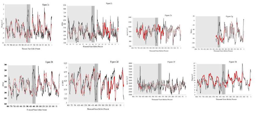
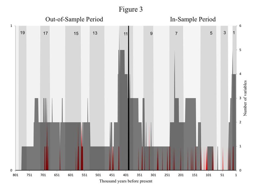
23

615 Figure Captions
616
617 Figure 1(a) Experimental data for the time series that responds quickly (T) that is generated by
618 the van der Pol Oscillator is given by the black line; the blue line represents values simulated by
619 the CVAR model. Figure 1(b) Experimental data for the time series that responds slowly (I) that
620 is generated by the van der Pol Oscillator is given by the black line; the blue line represents values
621 simulated by the CVAR model.
622
623 Figure 2 The observed values for temperature (black line) and values simulated by the system
624 model conditioned only on the four variables for solar insolation (red line). Thick portions of the
625 red line represent time steps in which the simulation error is significantly different from zero
626 (non-zero error). Red circles represent time steps when the simulation error is an (innovational)
627 outlier. The light gray area is the out-of-sample forecast period; MIS 11 is shaded dark gray. (b)
628 same as above for carbon dioxide, (c) same as above for methane, (d) same as above for land ice,
629 (e) same as above for Na, (f) same as above for SO4, (g) same as above for sea level, (h) same as
630 above for SST2.
631
632 Figure 3 The number of outliers (red spikes) and non-zero errors (darkly shaded) for each time
633 step. Marine isotope stages are indicated by alternating areas of shading.
634

 2
 Note that the series of SST exhibits non-zero simulation errors nearly throughout the sample, suggesting a non-
 zero bias throughout the observational record – simulated model values persistently exceed observations.

Figures

Figure 1

1(a) Experimental data for the time series that responds quickly (T) that is generated by the van der Pol
Oscillator is given by the black line; the blue line represents values simulated by the CVAR model. Figure
1(b) Experimental data for the time series that responds slowly (I) that is generated by the van der Pol
Oscillator is given by the black line; the blue line represents values simulated by the CVAR model.

Figure 2

The observed values for temperature (black line) and values simulated by the system model conditioned
only on the four variables for solar insolation (red line). Thick portions of the red line represent time steps
in which the simulation error is signi cantly different from zero (non-zero error). Red circles represent time
steps when the simulation error is an (innovational) outlier. The light gray area is the out-of-sample
forecast period; MIS 11 is shaded dark gray. (b) same as above for carbon dioxide, (c) same as above for
methane, (d) same as above for land ice, (e) same as above for Na, (f) same as above for SO4, (g) same
as above for sea level, (h) same as above for SST2.

Figure 3

The number of outliers (red spikes) and non-zero errors (darkly shaded) for each time step. Marine
isotope stages are indicated by alternating areas of shading.

Supplementary Files
This is a list of supplementary les associated with this preprint. Click to download.

KaufmannPretisSupporting.pdf
Table1.pdf
Table2.pdf
Table3.pdf