Delta-change approach for CMIP5 GCMs - Astrid Ruiter De Bilt, 2012 | Trainee report - KNMI
←
→
Page content transcription
If your browser does not render page correctly, please read the page content below
Delta-change approach for CMIP5 GCMs
Astrid Ruiter

                     De Bilt, 2012 | Trainee report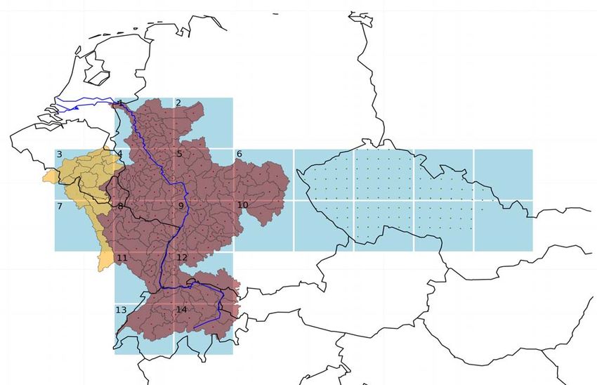
Delta-change approach for CMIP5 GCMs

Version   3

Date      September 2012
Status    Final

Delta-change approach for CMIP5 GCMs Internship report September, 2012 KNMI – Royal Netherlands Meteorological Institute Astrid Ruiter 3232158 Master student Quaternary Geology and Climate Change Department of Physical Geography UU – Utrecht University Under supervision of: Jules Beersma (KNMI) Adri Buishand (KNMI) Raymond Sluiter (KNMI) Maarten Zeylmans van Emmickhoven (UU) Version 3 Koninklijk Nederlands Meteorologisch Instituut Universiteit Utrecht PO Box 201, 3730 AE De Bilt, The Netherlands P.O. Box 80020, 3508 TA Utrecht, The Netherlands Visiting address: Wilhelminalaan 10 Visiting adress: Budapestlaan 4 Telephone +31 30 22 06 911 Telephone + 31 30 253 3550 www.knmi.nl www.uu.nl
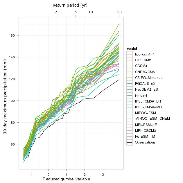
Table of Contents
Preface...................................................................................................................................................................3
1. Introduction ........................................................................................................................................................4
    1.1 Study area...................................................................................................................................................5
    1.2 Observation data.........................................................................................................................................6
    1.3 Global climate model data..........................................................................................................................6
2. Delta change method ........................................................................................................................................9
    2.1 Advanced delta change method ................................................................................................................9
    2.2 Interpolation to a common grid..................................................................................................................11
3. Results ...........................................................................................................................................................15
    3.1 Delta change method for 5-day precipitation sums..................................................................................16
    3.2 Return periods for maximum 10-day precipitation sums..........................................................................19
4. Discussion........................................................................................................................................................21
5. Conclusions & Future work..............................................................................................................................22
References...........................................................................................................................................................23
Appendix A: 90% quantiles of the CanESM2 and HadGEM2-ES models...........................................................26
Appendix B: Summary table for the summer period............................................................................................29
Appendix C: Gumbel distribution for calculation of return periods.......................................................................30

                                                                                   -2-                         Internship Report - Astrid Ruiter - 2012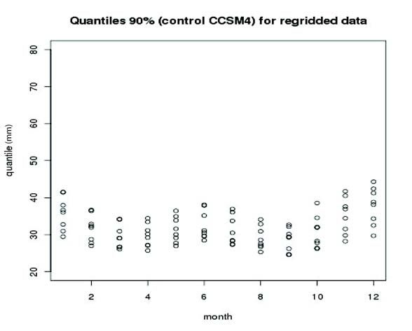
Preface

This report is written as a summary of the internship of Astrid Ruiter at the Royal Netherlands
Meteorological Institute (KNMI) at the department of climate data and climate advice (KS-KA). This
internship has been the final part of the master in Physical Geography at the University of Utrecht. The
goal of this internship was to perform an individual research project, as a part of a larger project at a
company or research institute to gain work experience.
This specific project is a continuation of a study of Saskia van Pelt, who is a PhD research student at
Wageningen University and partly at KNMI. In the paper of Van Pelt et al., 2012, the method and her
results are described. However, this is an internship report and it therefore only describes the method
briefly, with some parts of the method which have been renewed or extended. Since more recent climate
model data have been used for this study, the results will be different from the results described by Van
Pelt et al., 2012, which will be described in the discussion. Also, the project is not finished yet. The project
will be continued by Philip Kraaijenbrink who will start his internship in September 2012.
This internship has been performed under supervision of Maarten Zeylmans (UU) and Raymond Sluiter
(KNMI). The project- and daily supervision has been carried out by Jules Beersma, in cooperation with
Adri Buishand, Saskia van Pelt and Alexander Bakker. I would like to thank all of them for their help with
the project and the interesting and pleasant time at the KNMI.

                                                       -3-              Internship Report - Astrid Ruiter - 2012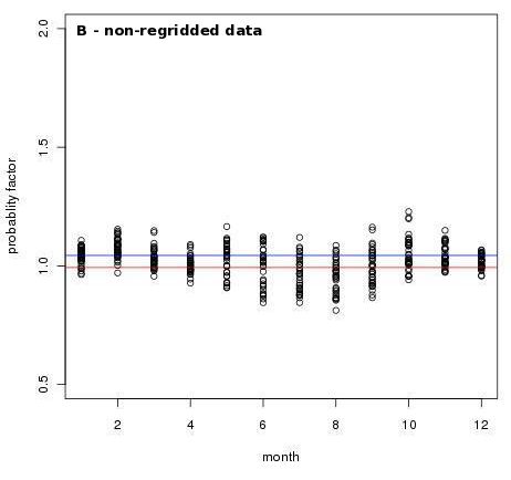
1. Introduction

The Netherlands has always been very vulnerable for high river discharges of the Rhine and Meuse
rivers, which dominate the environment of the Netherlands as well as the upstream area. More than 50
million people live in the catchments of Rhine and Meuse and both are also very important for economic
purposes as busy waterways (Disse and Engel, 2001). Therefore precipitation analysis are of major
importance for economic and flood-risk assessment at present and for future protection. Most climate
models show future changes in precipitation amount and distribution. Differences in temporal distribution
could mean that the seasonal precipitation spread will change, which can result in dryer summers and
wetter winter periods for the Rhine-Meuse area, or in an increase in extreme precipitation events (Frei et
al., 2006; Fowler and Ekström, 2009). Most of the climate models show similar changes in temperature
for northwestern Europe but changes in (extreme) precipitation are somewhat more uncertain (Frei et al.,
2006; Reichler and Kim, 2008; Kysely and Beranova, 2009; Kysely et al., 2011).

This study describes an extended application of the advanced delta change method introduced by Van
Pelt et al. (2012). The method is different from earlier delta change methods because it allows changes in
extremes to be different from changes in the mean. Van Pelt et al. (2012) describe this method in detail
and show the results of the future changes in extreme precipitation from RCM (Regional Climate Models)
and GCM (Global Climate Models) ensembles of the CMIP3 (Coupled Model Intercomparison Project)
models. The study of Van Pelt et al. (2012) shows the results of the method and a comparison between
individual RCM outputs and the signal of the driving GCMs. In this study, a new generation of GCMs (for
the CMIP5) has been used for the application of the advanced delta change method. In addition to the
application to a newer generation of GCMs, the Meuse catchment area has been added to the study
area. The method itself has not been changed but new research questions were formulated which this
study tries to answer:

   –   Will the new generation of GCMs give significantly different results in future precipitation changes
       compared to the previous used models?
   –   Which GCMs show the largest and which the smallest changes in (extreme) precipitation?

   –   What is the effect of interpolation to a common grid on the extreme precipitation values?
   –   What is a suitable common grid for the Rhine-Meuse basin, given the spatial resolution of the
       CMIP5 GCMs and the study area?

The delta-change approach is a method to “downscale” global climate model data in order to use it as a
future input for hydrological models and flood risk assessment. Different methods have been developed
for downscaling climate models to use for precipitation and discharge calculations (Prudhomme et al.,
2002; Te Linde, 2010). The advanced delta change method is a relatively simple and cheap method to
use global or regional climate models for extreme precipitation changes in a smaller scale area
(catchment scale) and use this information for changes in discharges and flood risk assessment for a
catchment scale area.

In the remaining part of this chapter, the study area and data are described. The input data, the
precipitation observations are described in section 1.2 and the global climate models (GCM) outputs are
described in section 1.3. Chapter 2 gives a brief description of methods; first the delta-change approach
in section 2.1, then the reason and testing method for assigning a common grid to the GCM data in
section 2.2. In chapter 3 the results are described and chapter 4 discusses these results. This report
ends with a conclusion about the method and the results and recommendations for future work.

                                                    -4-              Internship Report - Astrid Ruiter - 2012
1.1 Study area

The river Rhine, with a total length of 1230 km, is the longest river of western Europe. The Rhine
originates in the Swiss Alps, and has a total basin area of 185 000 km2. It is fed by glacier melt, snow
melt and rainfall. The annual mean discharge (calculated over 1901-2000) at Lobith is 2 200 m3 s-1 and
the discharge corresponding the Dutch design discharge, an estimated 1250-year return level, is 16 000
m3 s-1. This level (originally established by the Becht Committee in 1977) is evaluated every 5-years as a
part of the flood protection management of the Delta Committee (Leander, 2009). In addition to the
Rhine, the Meuse area is included in this study. The river Meuse originates on the plateau of Langres in
northeastern France and is mainly fed by rainfall. The total basin area upstream of Borgharen is 21 000
km2.

Although in this study the advanced delta change method is applied to the Rhine and Meuse basins, it
can be applied elsewhere as long as daily precipitation and temperature observation data, with sufficient
spatial density, are available. At the time of writing, there are plans to collaborate with German and Czech
partners. Some preparations have already been taken to apply the same method and the same GCMs, to
other large river basins relevant for Germany and the Czech Republic.

Figure 1: (A) The Meuse catchment with 15 individual subcatchments (after; Leander, 2009) and (B) the Rhine
area with a total of 134 subcatchments (after; De Wit and Buishand, 2007). Note that in some older literature
a different numbering is used for the Meuse basin.

                                                     -5-              Internship Report - Astrid Ruiter - 2012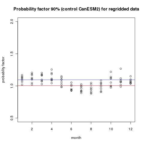
1.2 Observation data
The delta-change approach requires observation data for the entire study area that serves as the basis
for the method. The CHR-OBS dataset (International Commission for Hydrology of the Rhine basin;
Eberle et al., 2005; De Wit and Buishand, 2007) have been used for the Rhine area. This dataset
consists of area-average daily mean precipitation observations aggregated to 134 sub-catchments that
can be used for hydrological modeling (by HBV; Hydrologiska Bryans Vattenblansavdelning) (Figure 1B).
The CHR-OBS dataset is available for the period 1961 - 1995.
The Meuse area is subdivided into 15 HBV sub-basins (Figure 1A). Daily area-average mean
precipitation observations for these sub-basins are available for the period 1961 - 2008. The data of
French and Belgium meteorological surveys have been collected and interpolated to the HBV sub-basins
by Buishand and Leander (2011).
Both Rhine en Meuse sub-catchments are combined into a single observation data-set. The period of the
total 149 sub-basins is from 1961 - 1995. This is a 35-year period, which includes two extreme
precipitation events in 1993 (December) and 1995 (January) (Ulbrich and Fink, 1995; Leander, 2009).
Observed and gridded precipitation and temperature data for the Czech Republic (CHMI-OBS) are
available via Martin Hanel (from Czech University of Life Sciences Prague) and can be used for the
planned future extension of this method to the Czech Republic.
1.3 Global climate model data
This study makes use of the GCM simulations from the CMIP5 archive. These are the latest GCM
simulations available and they are analyzed for the upcoming IPCC assessment report (due 2013). Van
Pelt et al. (2012) used GCM simulations from the previous CMIP version (i.e. CMIP3). To explore different
possible futures the GCMs are 'forced' with different emission scenarios (which in turn depend on on
different scenarios for socio-economic development and mitigation policies). Both in this study and Van
Pelt et al. (2012), a single forcing was used. In this study the so called RCP4.51 (Representative
Concentration Pathways; Meinshausen et al., 2010) and in Van Pelt et al. (2012) the SRES (Special
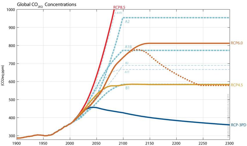
Report on Emission Scenarios, IPCC) A1B emission scenario. Figure 2 compares for the different SRES
and RCP forcings the corresponding CO2 concentration as a function of time. Note that SRES A1B and
RCP4.5 differ significantly in CO2 concentration at the year 2100 (590 CO2 eq. ppm for RCP4.5 vs. 780
CO2 eq. ppm for the SRES A1B scenario). It is expected that these differences will also lead to
differences in the results in this study and those in Van Pelt et al. (2012).
1 The 4.5 in RCP4.5 refers to a radiative forcing of 4.5 W/m2 (based on a medium mitigation scenario,
Taylor et al., 2009).
-6- Internship Report - Astrid Ruiter - 2012Figure 2: Comparison in terms of equivalent global CO2 concentrations of SRES emission scenarios (B1, B2,
A1T, A1B, A1F1, A2) used in CMIP3 simulations and RCPs (RCP-3PD, RCP4.5, RCP6.0 and RCP8.5) used
as forcings for CMIP5 simulations (Lee, 2011).
A total of 38 out of 109 available RCP4.5 GCM model runs has been used in this study. The total of 38
model runs consists of 15 different GCM simulations with each between 1 and 9 model runs (Table 1).
Daily precipitation data of the 38 model runs were all available for the three periods, commonly used in
hydrological modeling; 1961-1995 (in a historical run), 2021-2050 and 2071-2100. In the remaining part
of this report the period 1961-1995 is referred to as the “control period” and the period 2071-2100 as the
“future period”. Note that the model data for the 2021-2050 period, was also made available and
prepared but not further used in this study.
The GCMs are all available in Cartesian latitude-longitude grid, but the grid size and grid cell reference
are different for each model. The majority of the models has a 365-day calender, which is also known as
'no leap' because leap days are not included and each year has 365 days. Some of the models have a
standard (gregorian) calender, which includes the leap days. The HadGEM2-ES GCM is the only model
which has a calender of 360 days.
The GCM model outputs are available via the CMIP5 website (CMIP5, by Taylor, 2012) in NetCDF-files
(Network Common Data Frame), which is a format that is easily usable for climate data, especially for
large datasets (Unidatal; Unidata Program Center, 2012).
-7- Internship Report - Astrid Ruiter - 2012Model Runs Calender Institution References
1 bcc-csm1-1 1 365-day Beijing Climate Center, China Meteorological Wu et al., 2010
Administration
2 CanESM2 5 365-day Canadian Centre for Climate Modelling and Analysis Chylek et al., 2011
3 CCSM4 2 365-day National Center for Atmospheric Research Gent et al., 2011
4 CNRM-CM5 1 Standard Centre National de Recherches Meteorologiques Voldoire et al., 2012
5 CSIRO-Mk3-6-0 9 365-day Commonwealth Scientific and Industrial Research Rotstayn et al., 2010
Organisationin collaboration with the Queensland
Climate Change Centre of Excellence
6 FGOALS-s2 3 365-day LASG, Institute of Atmospheric Physics, Chinese Juan et al., 2008
Academy of Sciences
7 HadGEM2-ES 4 360-day Met Office Hadley Centre Collins et al., 2011
8 inmcm4 1 365-day Institute for Numerical Mathematics Volodin et al., 2010
9 IPSL-CM5A-LR 4 365-day Institut Pierre-Simon Laplace Dufresne et al., 2012
10 IPSL-CM5A-MR 1 365-day Institut Pierre-Simon Laplace Dufresne et al., 2012
11 MIROC-ESM 1 Standard Japan Agency for Marine-Earth Science and Watanabe et al., 2011
Technology, Atmosphere and Ocean Research Institute
12 MIROC-ESM- 1 Standard Japan Agency for Marine-Earth Science and Watanabe et al., 2011
Technology, Atmosphere and Ocean Research Institute
CHEM
13 MPI-ESM-LR 3 Standard Max Planck Institute for Meteorology Raddatz et al., 2007;
Jungclaus et al., 2010
14 MRI-CGCM3 1 Standard Meteorological Research Institute Yukimoto et al., 2011
15 NorESM1-M 1 365-day Norwegian Climate Centre Kirkevag et al., 2008;
Seland et al., 2008
Table 1:Different GCM simulations used in this study.
-8- Internship Report - Astrid Ruiter - 20122. Delta change method
The delta change approach is a method that makes the output of GCMs useful for catchment scale
analysis and hydrological modeling (which means that the GCM outputs are used indirectly). The method
is based on the use of a change factor, the ratio between a mean value in the future and historical run.
This factor is then applied to the observed time series to transform this series set into time series that is
representative of the future climate.
2.1 Advanced delta change method
In the classical delta change method the transformation of the historical data makes only use of to
changes in mean values. However, for flood risk assessments, for which extreme precipitation events are
very important, the changes in the extremes, which may be different from those in the mean, should be
taken into account as good as possible.
The advanced delta change method consists of a non-linear transformation of historical precipitation
data. The advanced delta method takes into account the changes in mean and in extremes, to extract the
climate signal from climate model outputs. This climate signal is applied on observation data to create a
(transformed) future dataset. In the advanced delta change method 5-day precipitation sums are the
starting point for the transformation. The 5-day sum is used to make the flood risk assessment possible,
as extreme discharges occur as a result of extreme multiple-day precipitation amounts. Extreme multi-
day sums between 4 to 20 days are considered to be relevant for the generation of extreme discharge for
the Rhine area. Another reason for using a 5-day sum has to do with the practical issue that one year of
365 days can be subdivided into 73 non-overlapping 5-day periods.
The observed 5-day precipitation amounts P are transformed using:
O
for PP90 : (1b)
Ē
In which P is an historical 5-day sum, P* the transformed (future) 5-day sum and a and b the
transformation coefficients (parameters). In all equations and figures PO and P* represent the observed
and transformed future precipitation data. Similar as the superscripts O and * represent the observed and
transformed data, the superscripts C and F are representative for the control and future climates. The P90
is the 90% quantile, which is the threshold for which 90% of the probability distribution is below this value.
EC and EF represent the excess variable of the control and future period of the GCMs. The amount E
above the 90% quantile is called the excess (Equation 2).
E = P – P90 (2)
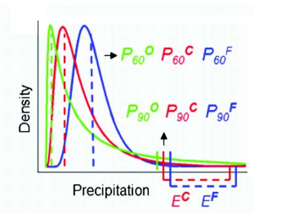
Figure 3 is a schematic representation of the probability distribution of 5-day precipitation amounts for the
observations and for the control and future GCM simulations together with their 60% and 90% quantiles
and Excess.
The theoretical background for Equation (1b) in which the transformed precipitation linearly scales with
the ratio of the future and control excess is given in Appendix A of Van Pelt et al. (2012). This linear
scaling also avoids that unrealistically large precipitation amounts are generated, especially when b is
larger than 1.
-9- Internship Report - Astrid Ruiter - 2012Similarly as for the 30% and 90% quantiles, 60% of the values are smaller than the 60% quantile. Note,
that because of the skewness of the precipitation probability distribution (Figure 3) the 60% quantile is
more representative for the mean than the median (which is the 50% quantile).
Figure 3: Schematic probability distribution of precipitation for
observations and control and future data of the GCM simulations (Van Pelt
et al., 2012).
The parameters a and b, which are used in Equation (1a and 1b), are calculated by the formulas (3) and
(4) by eliminating a and then substituting b in Equation (1a).
log { g 2 P 90 )}
F F
/( g 1 P 60
b= (3)
log { g 2 P 90 /( g 1 P 60) }
C C
/(P C60 )b g (1−b)
F
a=P 60 1 (4)
Correction factors (g1 and g2) are needed in Equation (3) and (4) and are calculated as:
O C
g1=P60 / P60 (5a)
g2=PO90 / PC90 (5b)
These correction factors are needed to account for systematic differences in the 60% and 90% quantiles
between the observations and the GCM control run and to ensure that in the transformation of the
observations the relative changes of P60 and P90 derived from the GCM are reproduced.
To make the transformation as flexible as possible, the transformation coefficients vary spatially and/or
seasonally. Therefore these coefficients are determined separately for each grid cell and each calender
month. To avoid sampling noise in these coefficients the underlying quantiles are smoothed by taking the
monthly mean data of one-fourth of the previous, one-fourth of the next and half of the concerning month.
To reduce sampling variability the median of b over all grid cells is uniformly used for all grid cells.
- 10 - Internship Report - Astrid Ruiter - 2012The mean excess for control and future periods, which is needed for the upper 10% of the probability
distribution (as used in Equation (1b)), is described by:
̄C ∑
E = C =
E C ∑ ( PC −P 90)
C
(6a)
n nC
∑ E F ∑ (P F −P 90F )
ĒF = F = (6b)
F
n n
In these equations EC and EF are the excesses of individual 5-day mums. nC and nF are the total number
of excesses for the current and future climate. The mean excesses ĒC and ĒF are smoothed over time in
a similar way as the quantiles.
The final step in the method is to apply a change factor to the daily observation data. The change factor
is represented by:
R= P* / P (7)
The change factor is calculated for each 5-day sum period and is applied for each day within the 5-day
period and is calculated for each grid cell separately. This way, a new data set of precipitation data was
generated for each GCM. The same change factor R is also applied to the individual sub-basins within a
grid-cell.
The entire method has been programmed in R, which is an open source software environment,
performed for statistical computing and graphics (R Development Core Team, 2005).
2.2 Interpolation to a common grid
It was already noted in the previous section that the different GCMs have varying resolutions. For ease of
comparison and to be able to use a common set of programs/scripts for applying the advanced delta
change method to each GCM it is desirable to make use of a common (interpolated) grid. This was also
done by Van Pelt et al. (2012) but they paid little attention to the fact that any interpolation smooths
extreme values and thus also has an effect on extreme quantiles that play an important role in the
advanced delta change method. This section describes the effect of interpolation on the individual
quantiles and more importantly, on the quantile factor. As a result of this analysis, a new interpolated
common grid was chosen. Figure 6 shows the new common grid boxes and the underlying 149
catchments of the concerning parts of the Rhine and Meuse area, which has been used as an input for
the advanced delta change method.
In general, interpolation to a common grid causes smoothing of data. In particular the extreme values are
smoothed, which in this study are of major importance. The effect of interpolation on the quantiles and
quantile factors (as used in the delta change method) was studied for three models with different grid
sizes. The three models used are: CanESM2 (grid size of 2.81 x 2.79 degree, a total of 9 grid cells),
CCSM4 (grid size of 1.25 x 0.94 degree, a total of 35 grid cells) and HadGEM2-ES (grid size of 1.875 x
1.25 degree, a total of 18 grid cells). The effect of interpolation was investigated using the common grid
of Van Pelt et al. (2012). This common grid contains 8 grid boxes and covers the Rhine area only.
Therefore, the regridded data consists of 8 spatially varying values.
In the analysis both regridded and non-regridded model outputs were used to calculate the 30%, 60%
and 90% quantiles for the control (1971-1995) and future (2071-2100) precipitation data. From this,
quantile factors (which is the ratio of a quantile between the future and control periods for each grid cell
and calendar month) have been calculated and compared.
- 11 - Internship Report - Astrid Ruiter - 2012A B
C D
Figure 4: 90% quantile (in mm precipitation) of the CCM4 model for the control (A and B) and future (C and D)
period. The left panels (A and C) show the results of the regridded data (1 value per grid per month for 8 grid
cells), the right panels (B and D) those for the results of the original 35 grid cells.
Figure 4 shows that for the CCSM4 model the individual 90% quantiles for the regridded data differ from
those for the original grid cells. The figure shows the differences between the quantiles of the regridded
and original data (A and C against B and D) but also the differences between control and future period (A
and B against C and D). The largest differences are found for the winter period (months 10, 11, 12, 1, 2
and 3) in which the 90% quantiles of the original data show values up to 75 mm, while after interpolation
these values are reduced to a maximum of only 45 mm. The difference between control and future
periods is very small. Because of this small difference, the quantile factor (Figure 5) is generally around
1.0, both for the regridding and non-regridded data. The differences between the quantile factors of
regridded and non-regridded values are relatively small, and especially the difference in the average for
the summer (red line) and winter (blue line) periods is very small. Because the quantile factor is used in
the transformation rather than the individual quantiles, the differences between the quantiles themselves
are not of major influence on the method.
- 12 - Internship Report - Astrid Ruiter - 2012Figure 5: 90% quantile factor of the CCM4 model. At the left graph (A), the results of the regridded data have
been shown. The right graph (B) shows the results of the original 35 grid cells. The blue line represents the
winter mean (both 1.044) and the red line the summer mean (1.000 vs. 0.993).
The 90% quantiles for the CanESM2 and HadGEM2-ES regridded and original data show similar results
and can be found in Appendix A.
These results, in combination with the desire to use a common grid for all GCMs, a new common grid of
1.2° latitude by 2° longitude was chosen. This grid is based on the mean size of all GCM grid resolutions
in relation to the Rhine and Meuse basins (and Czech Republic). A grid with too large grid cells will have
a too low spatial resolution which diminishes the ability to distinguish regional differences within the
region of application. On the other hand, when the grid size becomes too small, an artificial accuracy will
be introduced.
For the common 1.2° latitude by 2° longitude grid, currently 8 grid cells on the x axis, ranging from 4° to
20° E and 5 grid cells on the y axis, from 46° to 52° N (Figure 6) were interpolated, covering the Rhine
and Meuse basins and the Czech Republic.
Only the westernmost 14 gridboxes, covering the Rhine and Meuse, were used in this study. The centroid
of the individual catchments determines to which gridbox it is assigned. One exception is made for the
most southern catchment of the Meuse (nr 1 in Figure 1A), which has been assigned to gridbox 7 as well,
even though the centroid of this gridbox is located just south of the gridbox.
The interpolation to the common grid cells was performed using the program CDO (Climate Data
Operators). This program has been developed by the Max-Planck-Institute for Meteorology of which
version 1.0.6 (December 2006) was used in this study. Ferret is a similar program which can be used and
has been used by Van Pelt (pers. comm.). This program uses the same interpolation technique (and
gives the same results), has useful parts by easy commands to show the changes in grid, and it makes
an automatic log-file. However, each model needs to be interpolated separately which increases the
amount of work and the chance of (typographic) errors. With CDO, the NetCDF-files were interpolated
using a standard bilinear interpolation technique (cdo remapbil) for the three selected time periods (1961-
1995, 2021-2050 and 2071-2100).
- 13 - Internship Report - Astrid Ruiter - 2012Figure 6: Study area with Rhine basin upstream from Lobith (red), Meuse basin upstream from Borgharen
(yellow) and Czech Republic (green dots) with common grid (blue boxes).
- 14 - Internship Report - Astrid Ruiter - 20123. Results
For the 38 RCP4.5 GCM simulations, the method was applied and a summary of the changes in the
30%, 60% and 90% quantiles and the excess is shown in Table 2. For completeness, the a and b
transformation coefficients and a performance index (PI) are included in this table.
WINTER run P30 P60 P90 Ē a b PI
1A bcc-csm1-1 r1i1p1 0,928 0,998 1,061 1,140 0,814 1,096 41,19
2A CanESM2 r1i1p1 0,795 0,892 1,014 1,117 0,652 1,162 3,44
2B CanESM2 r2i1p1 0,917 0,987 1,083 1,175 0,803 1,120 3,44
2C CanESM2 r3i1p1 0,897 0,972 1,026 1,191 0,843 1,100 3,44
2D CanESM2 r4i1p1 0,826 0,881 0,987 1,161 0,632 1,181 3,44
2E CanESM2 r5i1p1 0,876 0,939 1,023 1,167 0,742 1,122 3,44
3A CCSM4 r1i1p1 0,884 0,934 0,976 1,077 0,827 1,092 9,03
3B CCSM4 r2i1p1 0,687 0,816 0,931 1,077 0,622 1,149 9,03
4A CNRM-CM5 r1i1p1 1,067 1,122 1,125 1,138 1,096 1,012 3,93
5A CSIRO-Mk3-6-0 r10i1p1 0,841 0,933 1,040 1,169 0,740 1,107 5,75
5B CSIRO-Mk3-6-0 r1i1p1 0,941 1,010 1,046 1,113 0,879 1,087 5,75
5C CSIRO-Mk3-6-0 r3i1p1 0,757 0,865 0,969 1,080 0,650 1,162 5,75
5D CSIRO-Mk3-6-0 r4i1p1 0,882 0,952 1,039 1,072 0,772 1,126 5,75
5E CSIRO-Mk3-6-0 r5i1p1 1,019 1,049 1,079 1,070 0,973 1,069 5,75
5F CSIRO-Mk3-6-0 r6i1p1 0,768 0,904 1,019 1,089 0,674 1,158 5,75
5G CSIRO-Mk3-6-0 r7i1p1 0,922 0,981 1,061 1,104 0,861 1,088 5,75
5H CSIRO-Mk3-6-0 r8i1p1 0,971 1,024 1,080 1,097 0,908 1,075 5,75
5I CSIRO-Mk3-6-0 r9i1p1 0,830 0,939 1,032 1,133 0,747 1,117 5,75
6A FGOALS-s2 r1i1p1 0,928 0,996 1,055 1,154 0,892 1,087 -
6B FGOALS-s2 r2i1p1 0,889 0,970 1,024 1,037 0,806 1,092 -
6C FGOALS-s2 r3i1p1 0,797 0,898 1,016 1,141 0,671 1,149 -
7A HadGEM2-ES r1i1p1 1,236 1,197 1,133 1,020 1,388 0,943 -
7B HadGEM2-ES r2i1p1 0,644 0,816 0,970 1,135 0,488 1,251 -
7C HadGEM2-ES r3i1p1 0,676 0,816 0,959 1,110 0,541 1,299 -
7D HadGEM2-ES r4i1p1 0,459 0,714 0,925 1,111 0,323 1,313 -
8A inmcm4 r1i1p1 0,880 0,936 1,020 1,145 0,775 1,098 19,72
9A IPSL-CM5A-LR r1i1p1 1,032 1,052 1,086 1,131 1,001 1,056 17,92
9B IPSL-CM5A-LR r2i1p1 0,694 0,824 0,970 1,161 0,558 1,182 17,92
9C IPSL-CM5A-LR r3i1p1 0,820 0,934 1,034 1,152 0,695 1,138 17,92
9D IPSL-CM5A-LR r4i1p1 0,962 0,970 1,028 1,161 0,812 1,129 17,92
10A IPSL-CM5A-MR r1i1p1 0,748 0,866 1,004 1,199 0,607 1,174 -
11A MIROC-ESM r1i1p1 1,025 1,098 1,077 1,105 1,107 1,005 29,37
12A MIROC-ESM-CHEM r1i1p1 0,977 1,038 1,057 1,103 0,999 1,033 30,39
13A MPI-ESM-LR r1i1p1 0,936 0,979 1,026 1,070 0,889 1,059 8,19
13B MPI-ESM-LR r2i1p1 0,983 1,035 1,047 1,134 0,968 1,042 8,19
13C MPI-ESM-LR r3i1p1 0,930 1,043 1,073 1,118 0,918 1,056 8,19
14A MRI-CGCM3 r1i1p1 1,031 1,073 1,084 1,110 1,020 1,027 3,14
15A NorESM1-M r1i1p1 0,880 0,969 1,058 1,162 0,798 1,094 -
MEAN GCM's 0,877 0,959 1,033 1,122 0,802 1,112 10,724
Min GCMs 0,459 0,714 0,925 1,020 0,323 0,943 3,140
Max GCMs 1,236 1,197 1,133 1,199 1,388 1,313 41,190
Table 2: Relative changes in 30%, 60% and 90% quantiles and mean excess (resp. P30, P60, P90 and
Ē) for the 5-day precipitation sum in winter, after transformation by delta change approach. Also the
change factors a and b are included in this table and a Performance Index (Wang, 2012) is shown in the
last column. The colours indicate the highest (red) and lowest (blue) 5 values of the variables.
- 15 - Internship Report - Astrid Ruiter - 20123.1 Delta change method for 5-day precipitation sums
Some of the results which are shown in Table 2 are plotted in Figure 7. In this figure, the 30%, 60% and
90% quantile factors (ratio between future and control period, respectively PF30/ PC30, PF60/ PC60 and PF90/
PC90) calculated directly from the GCMs are plotted against those calculated from the transformed
observations. The different numbers represent the different GCMs and their model runs, the labels are
shown in the first column of Table 2. The graph shows an almost perfect correspondence in all three
quantile factors. This means that the applied transformation reproduces the future changes in these
quantiles very well. Particularly in summer, the relation is stronger for the 60% and 90% quantile than for
the 30% quantile (see Figure 7 and 8). This is likely a result of the delta change transformation, in which
the 30% quantile is not explicitly used.
1,3
A P30 winter 7A
1,2
1,1 4A
9A
5E14A 11A
1,0 13B
12A
5H
9D 5B
13A
1A
2B 5G 6A 13C
0,9 2E 3A6B2C
5D15A
8A
Pf/Pc
2D 9C 5A
5I
0,8 6C
2A
10A 5C5F CMIP5
0,7 9B3B
7C
7B Lineair (CMIP5)
0,6 1:1 line
0,5
7D
0,4
0,4 0,5 0,6 0,7 0,8 P* 0,9 1,0 1,1 1,2 1,3
1,2 P60 winter 7A
B 4A
1,1 11A
14A
9A
5E
13C
12A
13B
1,0 5B5H
1A
6A
2C
6B
9D
15A 2B
5G
13A
Pf/Pc
2E5D
5I
8A
3A
9C
5A
0,9 5F
6C
2A
5C2D
10A CMIP5
3B
7B9B
7C Lineair (CMIP5)
0,8
1:1 line
0,7 7D
0,7 0,8 0,9 P* 1,0 1,1 1,2
1,2 P90 winter
C
7A
4A
1,1 5H9A
14A
2B
5E
11A
5A 5G
5D
9C 6A 13C
1A
15A
12A
13B
5B
5I
8A
5F
6C
2A 9D
2C
13A
6B 2E
1,0 10A2D
7B3A
9B5C
Pf/Pc
7C
3B7D
0,9
CMIP5
0,8 Lineair (CMIP5)
1:1 line
0,7
0,7 0,8 0,9 P* 1,0 1,1 1,2
Figure 7: The 30%, 60% and 90% quantile factor (the ratio between Pf and Pc) vs the transformed
observation data for the winter period. Note the differences in scale.
- 16 - Internship Report - Astrid Ruiter - 2012Winter
The mean of PF90/ PC90 for all GCM's (see Table 2) for the winter period is 1.03, which means an increase
in the precipitation 90% quantile of 3%. The five lowermost model results are highlighted in blue, and the
five highest values in red. An interesting result is that the HadGEM2-ES model shows the most variety
and gives the minimal as well as maximal values for PF90/ PC90, run 4 (7D in Figure 7) has the lowest value
of 0.925 while run 1 (7A in Figure 7) results in the highest value of 1.13.
The 60% quantile is a representative value of the mean of the precipitation distribution. A value below 1
means that the total mean in precipitation will decrease in the future. Table 2 shows a value of 0.959, i.e.
a decrease of 4,1%, for the 60% quantile in winter. Both 30% and 60% quantiles show a decrease in
quantile factor (Figure 7A and 7B). The decrease in 30% quantile factor means that the driest parts of the
precipitation distribution will become dryer. This 30% quantile has been included in the analysis to get a
better insight in the dry part of the probability distribution of the precipitation. Since the results in Table 2
show a non-linear change in quantiles, the non-linear transformation is justified.
Summer
The PF90/ PC90 for the summer period (Figure 8, and the Table in Appendix B) shows a larger increase than
for the same quantile averaged over all GCMs for the winter period; 1.09, an increase of 9% vs an
increase of 3% for the winter period (Table 2). All models show an increase in the 90% quantile factor for
the summer period, ranging from 1.03 for an IPSL-CM5A model to a maximum value of 1.13 for the
HadGEM2-ES model, run 2 and 3 (7B and 7C). In comparison with the winter period, the inter model
range between the different quantile factors is much smaller during the summer period (note the
differences in scale of the x-axis between winter and summer (respectively Figures 7 and 8). The change
in quantile factors of P30 and P60 are similar to those for P90. The summer period shows higher values
(i.e. larges increases) and a smaller range between the different models.
The changes in the mean excess (Ē) are shown in Table 2. The mean increase in the excess in winter is
12.2%, with an overall range between + 2% and almost 20%. So in contrast to the changes in the
quantiles (i.e. the quantile factors) no decreases are found for any of the models. The highest value for
excess is by IPSL-CM5A-MR model, which is 1.199, while the lowest value for excess is 1.020 by the first
run of the HadGEM2-ES model.
The range in the resulting values, for both summer and winter period (Table 2), increase from excess,
towards the quantiles 90%, 60% and 30%. This means that the uncertainty increases towards the 30%
quantile. The total range of the 30% quantile is 0.777, which results in quantiles vary from 0.459 for the
HadGEM2-ES model (run 4) towards 1.236 for the HadGEM2-ES model (run 2). As well for the 90% and
60% quantiles, the HadGEM2-ES shows the largest variability. The excess shows a different pattern.
With exception of HadGEM2-ES run 1, all HadGEM2-ES model runs show similar values.
As expected large increases (decreases) of P60 and P90 typically correspond to large (low) values of a.
And, large (small) differences between the changes of P60 and P90 lead to values larger than (close to)
1. Quite often large values of a are accompanied by low values of b and vice versa. From this we may
conclude that the largest increases op P60 and P90 are more linear in character than the largest
decreases of P60 and P90. A similar result is also found for the summer period (see Appendix B). At this
moment we don't have a logical explanation for this negative correlation between the parameters a and b.
The Performance Index (PI) is a method of Wang, (2012), to order the different GCMs in their
performance (the models that represent the current climate best have the lowest values). Wang (2012)
shows how well the GCMs can reproduce the present climate to be able to order the results of the
different GCMs for the KNMI next scenarios. Not all models used by Wang (2012) are included in this
study and vice versa. The values in the last column of Table 2 represent PI values of Wang (2012),
averaged over the winter period. Every model is represented by one single value and no difference in
model runs have been made. Unfortunately, the HadGEM2-ES model is not included in the study of
Wang (2012), which would have been very interesting because this model shows the largest variation
- 17 - Internship Report - Astrid Ruiter - 2012within the results. The table does not show a correlation between PI values and any of the other results in
Table 2.
1,3
P30 summer
A 7B
1,2
1A
6B7C5E 5H
12A
5I11A
1,1 13B 13A
2C 2A 7D 14A
Pf/Pc
9D3A3B 6C 4A
5B 6A5C10A
1,0 2D 5D 7A 13C
5F 5A 15A CMIP5
9B 9A 2B 8A
5G Lineair (CMIP5)
2E
0,9 9C
1:1 line
0,8
0,8 0,9 1,0 1,1 1,2 1,3
P*
B P60 summer
1,2
7B
5H
7C
6B5E
1A
5I
11A
1,1 13B
12A
14A
7D
13A
4A
2C
3A
10A
9D
Pf/Pc
6C
13C
3B
5B
2A
5C
6A
15A CMIP5
8A
5D7A
5A
5F Lineair (CMIP5)
1,0 2B9A
2D
9B
5G 1:1 line
9C2E
0,9
0,9 1,0 P* 1,1 1,2
C P90 summer
1,2
2C
3A 7B 7C
6B
5H
9D
1A 10A
5E7D
1,1 12A11A
13B
5I
9A9B
13A
6C 5B14A
3B
15A
5F 6A 7A
5A
13C
Pf/Pc
5G 2A
2D
4A 5C
8A5D
2B2E
9C CMIP5
Lineair (CMIP5)
1,0
1:1 line
0,9
0,9 1,0 P* 1,1 1,2
Figure 8: The 30%, 60% and 90% quantile factor (the ratio between Pf and Pc) vs the transformed
observation data for the winter period. Note the differences in scale.
- 18 - Internship Report - Astrid Ruiter - 2012Table 3 shows the results of the analysis of the CMIP3 models by Van Pelt et al. (2012). This shows for
the 90% quantile a mean change of 8.5%.
The CMIP3 data, which are forced by the A1B emission scenario, (Van Pelt et al., 2012) show an
increase in P90 for all models. This is in contrast to the CMIP5 data, which are forced by a RCP4.5 forcing,
in which 8 out of the 38 models show a decrease in 90% quantile of the precipitation. The mean change
of the winter 90% quantiles of all GCMs for the CMIP3 is also higher than for the CMIP5 GCMs (8.5% vs.
3%). The range between the different model outputs is for all variables (PF60/ PC60 and PF90/ PC90) smaller
for the CMIP3 results compared to the CMIP5 results.
WINTER P60 P90 Ē
CGCM3.1T63 1,1 1,11 1,22
CNRM-CM3 0,97 1,04 1,28
CSIRO-Mk3.0 1,01 1,05 1,17
ECHAM5r1 0,98 1,04 1,25
ECHAM5r3 1,11 1,15 1,11
GFDL-CM2.0 1,04 1,11 1,21
GFDL-CM2.1 1,05 1,1 1,41
HADCM3Q0 1,12 1,17 1,35
HADCM3Q3 1,07 1,12 1,2
IPSL-CM4 0,89 1,01 1,36
MIROC3.2 0,94 1,03 1,19
MIUB 0,95 1,09 1,24
MRI-CGCM2.3.2 1,05 1,09 1,34
Table 3: Relative changes in 60% and 90% quantiles and
mean excess (resp. P60, P90 and Ē) for the 5-day
precipitation sum in winter, based in CMIP3 A1B
simulations (after; Van Pelt et al., 2012).
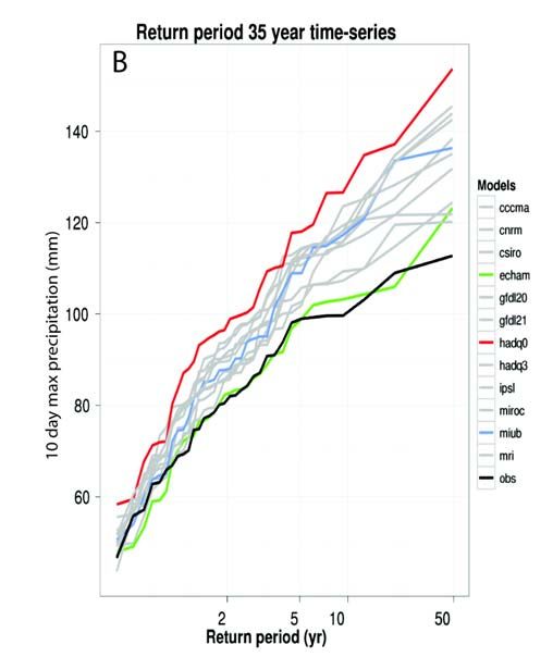
3.2 Return periods for maximum 10-day precipitation sums
Return level plots of the maximum 10-day precipitation for the CMIP5 GCMs used in this study are shown
in Figure 9A. A similar figure for the CMIP3 simulations used by Van Pelt et al. (2012), is given in Figure
9B. The 10-day annual maxima are in both figures derived from the transformed historical time series
(using the advanced delta change method). Note that in these plots, the horizontal axis, i.e. the return
period, corresponds to the scale of a Gumbel distribution (see Appendix C for details).
Both graphs show a very similar change in higher values and a larger range between the values for the
longer return periods. For the CMIP3 GCMs, the 50 year return period is between 110 and 150 mm for
the different model runs. For the CMIP5 GCMs this value ranges from 120 up to 170 mm. The largest 10-
day precipitation amounts are generated by the HadQ0 model for CMIP3 and the CSIRO-Mk3-6-0 for the
CMIP5 GCMs. Although both types of model simulations show similar changes in future return levels, a
proper comparison between the future return levels of the 10-day precipitation maxima of the CMIP5 and
CMIP3 simulations can not be made because: a) The CMIP3 A1B and CMIP5 RCP4.5 simulations differ
in climate forcings (i.e. CO2 concentration, see Figure 2) and b) the 10-day precipitation amounts in this
- 19 - Internship Report - Astrid Ruiter - 2012study involve both the Rhine and Meuse basins while the 10-day precipitation amounts in Van Pelt et al.
(2012) refer to the Rhine basin only. The precipitation in the Meuse area is a little higher than in the Rhine
basin which causes the 50-year return level of the observations (the black lines) to decrase form 119 mm
in panel A to 113 mm in panal B.
A
Figure 9: (A) Return levels of 10-day maximum precipitation amounts for CMIP5 RCP4.5 simulations and (B)
CMIP3 A1B simulations (after Van Pelt et al., 2012) for the end of the 21st century compared with the return
levels for the observations (the black line).
- 20 - Internship Report - Astrid Ruiter - 20124. Discussion
The advanced delta change approach resulted in a reliable transformed observation dataset for the future
period representative of 2071 and 2100. All 38 analyzed CMIP5 RCP4.5 GCM simulations show an
increase in extreme precipitation around 2100. The 50-year return levels for 10-day precipitation sums
are around 140 mm. For the CMIP3 A1B scenarios (Van Pelt et al., 2012) these 50-year return levels
show a mean in max 10-day precipitation sum are around 10% lower. The individual quantile factors of
the 60% and 90% and the excess values (Table 2) show a decrease in winter mean for CMIP5 in
comparison with the CMIP3 results. Even though the mean winter precipitation in this study is lower,
compared to the study of Van Pelt et al. (2012), it still shows a mean increase in extreme precipitation of
12%.
Except for the differences between the CMIP3 and CMIP5 model simulations (see legend of Figure 9),
more differences are present between the results of this study and the study of Van Pelt et al. (2012).
This study is based on a larger study area. Except from having another reference observation dataset,
the model outputs are regridded with a larger area which extend more towards the west. This might
change the total precipitation amounts and could include more oceanic influences. However, this effect is
presumably neglectable since the study area is large enough to smooth these small changes. This
difference in study area causes an extra variability between both studies. For correct comparison
between CMIP3 and CMIP5 climate models, the results of this study should be split between the Rhine
and the Meuse catchments.
During this study a start has been made for using the 30% quantile for the method. This may provide a
better insight in the dry part of the precipitation probability distribution. Although the future change in the
30% quantile is not an explicit element in the non-linear transformation, it is still considered useful to
analyze the reproduction of P30 in the transformed historical series since it gives an idea about how well
the transformation works for the dryer (less wet) part of the precipitation probability distribution.
Especially for GCM simulations in which there is a large reduction of precipitation (i.e. in summer drying).
The plume of the extreme 10-day precipitation amounts (Figure 9) is a useful way to show the variations
between all different models (in this study for only one emission scenario). When all available models are
included in this plume, the entire CMIP5 range of precipitation change will be covered. For hydrological
modeling, using this extreme multi-day precipitation plume, only a small nummer of the CMIP5 model
simulations can be selected to cover the entire range of climate models.
- 21 - Internship Report - Astrid Ruiter - 20125. Conclusions & Future work
– The new generation of GCMs shows different results in future precipitation changes compared to
the previous used models. The mean of the changes in excess, 90% and 60% quantiles are all
lower for the CMIP5 climate model simulations (RCP4.5) than for the CMIP3 simulations (SRES
A1B). This difference is at least partly caused by the difference in climate forcing. In contrast, the
for the 10-day precipitation the largest return levels estimated are higher for the CMIP5 models
than for CMIP3.
– The HadGEM2-ES model runs show the most extreme values for changes in 30%, 60% and 90%
quantiles and excess, and therefore the largest changes in extreme precipitation.
– The effect of the interpolation to a common grid is significant for the individual quantiles, but for
the quantile factors this effect is almost negligible. The advanced delta change method only uses
the quantile factors and therefore the effect of interpolation to a common grid on the extreme
precipitation values is not significant.
– A suitable common grid for the Rhine-Meuse basin and the Czech Republic, given the spatial
resolution of the CMIP5 GCMs and the study area, has been chosen. This grid has a resolution
of 1.2° longitude by 2° latitude (close to the average of all available GCMs) and is shown in
Figure 5.
More research is needed to be able to use the 10% and 30% quantiles which might be relevant to adapt
the advanced delta change method for drought studies.
The application of the advanced delta change method to other river basins including the use of CMIP5
GCM simulation forced by the other RCPs will be performed by the next intern. He will continue this study
and generate time series to be used together with the next generation of KNMI climate scenarios (due
autumn 2013) and especially for hydrological modeling purposes (in collaboration with RWS-Waterdienst
and Deltares). To prepare the transformed (future) time series for hydrological modeling, the following
subjects must be studied;
– The method must be extended with and applied to temperature data to be able to use the results
for hydrological modeling.
– Include leap days in the transformed historical data-set to complete the time series (the scripts of
Van Pelt (pers. comm.) already have this option).
– Apply the transformation on long term (3 000 to 20 000 year) precipitation data sets, which are
generated by the KNMI-rainfall generator.
– Apply the method for the future period 2021-2050 and compare these results with the period
2071-2100. This might give more insight in the direct effect of different forcings.
– Distinguish between the results for the Rhine and Meuse catchments for better comparison
between the changes for the delta change method based on CMIP3 (SRES A1B) and CMIP5
(RCP4.5) climate model simulations.
– Apply the advanced delta method on a other river basins and investigate the effect of using an
average b parameter with an larger study area.
– Apply the advanced delta method on other GCM simulations (for example RCP6.0) for better
comparison between CMIP3 and CMIP5 and the effect of different forcings and to cover the entire
range of the climate signal.
- 22 - Internship Report - Astrid Ruiter - 2012References
Aalders, P., Warmerdam, P.M.M. and Todfs, P.J.J.F., 2004. Rainfall generator for the Meuse Basin; 3,000
year discharge simulations in the Meuse basin. Wageningen University, sub-department water resources;
Report 124.
Bernstein, L., Bosch, P., Canziani, O., Chen, Z., Christ, R., Davidson, O., Hare, W., Huq, S., Karoly, D.,
Kattsov, V., Kundzewicz, Z., Liu, J., Lohman, U., Mannin, M., Matsuno, T., Mene, B., Metz, B., Mirza, M.,
Nicholls, N., Nurse, L., Pachauri, R., Palutikof, J., Parry, M., Qin, D., Ravindranath, N., Reisinger, A., Ren,
J., Riahi, K., Rosenzweig, C., Rusticucci, M., Schneider, S., Sokona, Y., Solomon, S., Stott, P., Stouff er,
R., Sugiyama, T., Swart, R., Tirpak, D., Vogel, C. and Yohe, G., 2007. Climate change 2007: Synthesis
report, Intergovernmental Panel on Climate Change (IPCC), Geneva, 1–52.
Buishand, T.A., and Leander, R., 2011. Rainfall generator for the Meuse; Extension of the base period
with the years 1999-2008. KNMI-publication; 196-V.
Chylek, P., Li, J., Dubey, M. and Lesins., G. 2011. Observed and model simulated 20th century arctic
temperature variability: Canadian earth system model canasm. Atmos Chem Phys Discuss 11: 22.
Collins, W.J., Bellouin, N., Doutriaux-Boucher, M., Gedney, N., Halloran, P., Hinton, T., Hughes, J., Jones,
C.D., Joshi, M., Liddicoat, S., Martin, G., O'Connor, F., Rae, J., Senior, C., Sitch, S., Totterdell, I.,
Wiltshire, A. and Woodward, S., 2011. Development and evaluation of an Earth-System model-
HadGEM2. GMD 4(4):1051-1075.
De Wit, M.J.M. and Buishand, T.A., 2007. Generator of Rainfall And Discharge Extremes (GRADE) for
the Rhine and Meuse basins. Rijkswaterstaat RIZA report 2007.027/KNMI publication 218. Lelystad, The
Netherlands.
Dissel, M., and Engel, H., 2001. Flood events in the Rhine basin: Genesis, influences and mitigation.
Natural Hazards, 23: 271-290.
Dufresne, J.L., Foujols, M.A., Denvil, S., Caubel, A. and Marti, O., 2012. Climate change projections
using the IPSL-CM5 earth system model: from CMIP3 to CMIP5. Clim Dyn.
Eberle, M., Buiteveld, H., Krahe, P. and Wilke, K., 2005. Hydrological Modelling in the River Rhine Basin,
Part III: Daily HBV model for the Rhine basin. Report 1451, Bundesanstalt für Gewasserkunde (BFG),
Koblenz, Germany, 2005.
Frei, C., Schöll, R., Fukutome, S., Schmidli, J. and Vidale, P.L., 2006. Future change of precipitation
extremes in Europe: Intercomparison of scenarios from regional climate models. Journal of geophysical
research, 111. 22 p.
Gent, P. R., Danabasoglu, G., Donner, L.J., Holland, M.M., Hunke, E.C., Jayne, S.R., Lawrence, D.M.,
Neale, R.B., Rasch, P.J., Vertenstein, M., Worley, P.H., Yand, Z.L. and Zhang, M., 2011. The Community
Climate System Model version 4. J. Climate.
Görgen, K., Beersma, J., Brahmer, G., Buiteveld, H., Carambia, M., de Keizer, O., Krahe, P., Nilson, E.,
Lammersen, R., Perrin, C. and Volken, D., 2010. Assessment of climate change impacts on discharge in
the Rhine river basin: Results of the RheinBlick2050 project, International Commission for the Hydrology
of the Rhine basin (CHR), Lelystad, Report no. I-23, 229 pp.
Juan, L., Bin, W., Hailong, L. and Yongqiang, Y., 2008. A New Global Four-Dimensional Variational Ocean
Data Assimilation System and its Application. Adv. Atmos. Sci., Vol. 25, NO. 4, 2008, 680-691.
- 23 - Internship Report - Astrid Ruiter - 2012Jungclaus, J.H., Lorenz, S.J., Timmreck, C., Reick, C.H., Brovkin, V., Six, K., Segschneider, J., Giorgetta,
M.A., Crowley, T.J., Pongratz, J., Krivova, N.A., Vieira, L.E., Solanki, S.K., Klocke, D., Botzet, M., Esch,
M., Gayler, V., Haak, H., Raddatz, T.J., Roeckner, E., Schnur, R., Widmann, H., Claussen, M., Stevens,
B. and Marotzke J., 2010. Climate and carbon-cycle variability over the last millennium. Clim Past
6(5):723-737.
Kirkevag, A., Iversen, T., Seland, O., Debernard, J.B., Storelvmo, T. and Kristjansson, J.E., 2008.
Aerosol-cloud-climate interactions in the climate model CAM-Oslo. Tellus A 60(3):492-512.
Kysely, J., and Beranova, L., 2009. Climate-change effects on extreme precipitation in central Europe:
uncertainties of scenarios based on regional climate models. Theor. Appl. Climatology 95: 361-374.
Kysely, J., Gaal, L., Beranova, R., Plavcova, E., 2011. Climate change scenarios of precipitation
extremes in Central Europe from ENSEMBLES regional climate models. Theor Appl. Climatology 104:
529-542.
Leander, R., and Buishand, T.A., 2007. Resampling of regional climate model output for the simulation of
extreme river flows. Journal of Hydrology, 332: 487-496.
Leander, R., 2009. Simulation of precipitation and discharge extremes of the river Meuse in current and
future climate. Proefschrift aan Universiteit Utrecht.
Lee, R., 2011. Extratropical storm tracks in some of the CMIP5 Models. Presentation University of
Reading.
Lenderink, G., Buishand, A., and Deursen, W., 2007. Estimates of future discharges of the river Rhine
using two scenario methodologies: direct versus delta approach. Hydrology & Earth System Sciences,
11(3): 1145-1159.
Meinshausen, M., Smith, S.J., Calvin, K., Daniel, J.S., Kainuma, M.L.T., Lamarqua, J-F., Matsumoto, K.,
Montzka, S.A., Raper, S.C.B., Riahi, K., Thomson, A., Velders, G.J.M. and van Vuuren, D.P.P., 2010. The
RCP greenhouse gas concentrations and their extensions from 1765 to 2300. Climate Change, 109: 213-
241.
R Development Core Team, 2005. A Language and Environment. R Foundation for Statistical computing,
Vienna, Austria. http://www.R-project.org.
Raddatz, T.J., Reick, C.H., Knorr, W., Kattge, J., Roeckner, E., Schnur, R., Schnitzler, K.G., Wetzel, P.
and Jungclaus, J., 2007. Will the tropical land biosphere dominate the climate-carbon cycle feedback
during the twenty-first century? Clim Dyn 29(6):565-574.
Prudhomme, C., Reynard, N. and Crooks, S., 2002. Downscaling of global climate models for flood
frequency analysis: where are we now? Hydrological Processes, 16: 1137-1150.
Reichler, T. and Kim, J., 2008. How Well Do Coupled Models Simulate Today's Climate? Bull. Amer.
Meteor. Soc., 89: 303-311.
Rotstayn, L., Collier, M., Dix, M., Feng, Y., Gordon, H., O'Farrell, S., Smith, I. and Syktus, J., 2010.
Improved simulation of Australian climate and ENSO-related climate variability in a GCM with an
interactive aerosol treatment. Int. J. Climatology, vol 30(7): 1067-1088.
Seland, O., Iversen, T., Kirkevag, A. and Storelvmo, T., 2008. Aerosol-climate interactions in the CAM-
Oslo atmospheric GCM and investigation of associated basic shortcomings. Tellus A 60(3): 459-491.
- 24 - Internship Report - Astrid Ruiter - 2012Taylor, K.E., 2012. Information about the CMIP5 experiments design and any CF and data output.
Program for Climate Model Diagpnosis and Intercomparison, LLNL. http://cmip-pcmdi.llnl.gov/cmip5/
Taylor, K.E., Stouffer, R.J. and Meehl, G.A., 2009. A Summary of the CMIP5 Experiment Design.
Program For Climate Model Diagnosis and Intercomparison.
Taylor, K.E., Stouffer, R.J. and Boer, G., 2010. Addendum to the CMIP5 Experiment Design Document: A
compendium of relevant emails sent to the modeling groups. Program For Climate Model Diagnosis and
Intercomparison.
Te Linde, A.H., Aerts, J.C.J.H., Bakker, A.M.R. and Kwadijk, J.C.J., 2010. Simulating low-probability peak
discharges for the Rhine basin using resampled climate modeling data. Water Resources Research, 46.
Ulbrich, U., and Fink, A., 1995. The January 1995 flood in Germany: Meteorological versus hydrological
causes. Phys. Chem. Earth 20, nr 5-6: 439-444.
Unidata Program Center, 2012. Providing innovative data services and tools to transform the conduct of
geoscience. Unidata Program Center, Boulder, CO, United States. http://www.unidata.ucar.edu.
Van Pelt, S.C., Beersma, J.J., Buishand, T.A., Van den Hurk, B.J.J.M. and Kabat, P., 2012. Future
changes in extreme precipitation in the Rhine basin based on global and regional climate model
simulations. Hydrology and Earth System Science Discussions, 9: 6533-6568.
Voldoire, A., Sanchez-Gomez, E., Salas y Melia, D., Decharme, B. and Cassou, C., 2011. The CNRM-
CM5.1 global climate model: description and basic evaluation. Clim Dyn.
Volodin, E.M., Diansky, N.A. and Gusev, A.V., 2010. Simulating present-day climate with the INMCM4.0
coupled model of the atmospheric and oceanic general circulations. Atmospheric and oceanic physics,
V.46, N4.
Wang, X., 2012. Performance Index (PI) analysis and bias of the CMIP5 models for the KNMI next
scenarios. KNMI-publications.
Watanabe, S., Hajima, T., Sudo, K., Nagashima, T., Takemura, T., Okajima, H., Nozawa, T., Kawase, H.,
Abe, M., Yokohata, T., Ise, T., Sato, H., Kato, E., Takata, K., Emori, S. and Kawamiya, M., 2011. MIROC-
ESM 2010: model description and basic results of CMIP5 20c3m experiments. GMD 4(4):845-872.
Wu, T.W., Yu, R.C., Zhang, F., Wang, Z., Dong, M., Wang, L., Jin, X., Chen, D. and Li, L., 2010. The
Beijing Climate Center atmospheric general circulation model (BCC-AGCM2.0.1): description and its
performance for the present-day climate. Clim Dyn 34: 123−147.
Yukimoto, S., Adachi, Y., Hosaka, M., Sakami, T., Yoshimura, H., Hirabara, M., Tanaka, T.Y., Shindo, E.,
Tsujino, H., Deushi, M., Mizuta, R., Yabu, S., Obata, A., Nakano, H., Ose T. and Kitoh, A., 2012. A new
global climate model of Meteorological Research Institute: MRI-CGCM3 - Model description and basic
performance. J. Meteor. Soc. Japan, Special Issue.
- 25 - Internship Report - Astrid Ruiter - 2012You can also read


