Spatial prediction of weed intensities from exact count data and image-based estimates.
←
→
Page content transcription
If your browser does not render page correctly, please read the page content below
Spatial prediction of weed intensities from exact count
     data and image-based estimates.

     Gilles Guillot
     INRA-AgroParisTech Applied Mathematics and Computer Science joint research unit, 16, rue
     Claude Bernard, 75231 Paris cedex 05 France, and Gothenburg Stochastic Centre, Chalmers
     University of Technology, SE 412-96 Gothenburg, Sweden. Now at Centre for Ecological and
     Evolutionary Synthesis, Department of Biology, University of Oslo, P.O Box 1066 Blindern,
     0316 Oslo Norway.
     Niklas Lorén
     SIK, The Swedish Institute for Food and Biotechnology, P.O. Box 5401, SE-402 29 Gothenburg,
     Sweden
     Mats Rudemo
     Department of Mathematical Statistics,Chalmers University of Technology, SE 412-96 Gothen-
     burg, Sweden

     Summary. Collecting weed exact counts in an agricultural field is easy but extremely time
     consuming. Image analysis algorithms for object extraction applied to pictures of agricultural
     fields may be used to estimate the weed content with a high resolution (≈ 1m2 ), and pictures
     acquired at a large number of sites can be used to get maps of weed contents over a whole field
     at a reasonably low cost. However, these image-based estimates are not perfect and acquiring
     also exact weed counts is highly useful both for assessing the accuracy of the image-based
     algorithms and for improving the estimates by use of the combined data. We propose and
     compare different models for image index and exact weed count and we use them to assess
     how such data should be combined to get reliable maps. The method is applied to a real data
     set from a 30 ha field. We show that using image estimates in addition to exact counts allows
     us to improve significantly the accuracy of maps. We also show that the relative performances
     of the methods depend on the size of the data set and on the specific methodology (full-Bayes
     versus plug-in) implemented.

    Keywords: spatial prediction, multivariate data, Gaussian random field, approximate
Cox process, Poisson regression, model based geostatistics, image analysis, precision farm-
ing.

1. Statistical approaches for weed mapping

The increased need to protect environment, in particular to avoid spreading chemical prod-
ucts where it is not necessary, has prompted farmers to develop practices adapted to the
characteristics of soil and vegetation at small scale in the field. Regarding the spread of
herbicides, varying the amount of product supplied locally requires a map of weed content
in the field at a fairly high resolution.
    The statistical approaches developed to obtain such maps may be based on exact weed
counts only. The earlier approaches to get maps from weed counts only have been based
on traditional geostatistical methods. Implementation of such methods can be found in
2 G. Guillot et al.
the works of Heisel et al. (1996), Rew and Cousens (2001), Rew et al. (2001), Dille et al.
(2002), where it is reported that simple interpolation procedures often behave poorly for
weed mapping when the number of samples available is restricted by economical constraints
(less than 10 data points per hectare).
Other methods based on the use of exact counts and auxiliary variables correlated with
the weed content such as organic matter in soil or remote sensing estimates have been
considered, see e.g. Heisel et al. (1999) and Lamb et al. (1999), but the improvement
compared to the use of exact counts only depends on the strength of the relationship between
exact counts and covariates which is usually rather low.
Strategies based on analysing pictures of the ground at small scale (≈ 1m2 ) to get
estimation of weed (or crop) content have been widely studied, see e.g. Marchant and
Brivot (1995), Brivot and Marchant (1996), Andreasen et al. (1997), Brivot and Marchant
c
(1998), Pðrez et al. (2000), Soille (2000), Tillet et al. (2001), Åstrand and Baerveldt
(2002), Onyango and Marchant (2003), Gerhards and Christensen (2003). In the previous
works, high resolution images are supposed to be available at an arbitrary site, hence, the
question of spatial interpolation is not tackled in these works; the accuracy of the image
estimates at a particular site is assessed by comparing its output to the weed content at
this particular site. However, in practice collecting and processing a very large number of
pictures can be prohibitive in terms of time, and visiting the whole field at a late growth
stage can damage the crop. Consequently, the question of how a large but limited number
(say up to a few tens per hectare) of such image-derived estimates should be used to get
interpolated maps should be addressed. Additionally, the quality of the estimation of weed
content by images only can vary a lot. Hence it can be informative to collect also exact weed
count data to assess the accuracy of the image analysis algorithm, and possibly to combine
exact count to image derived estimates in the interpolation scheme to increase its accuracy.
The aim of the present paper is to propose and implement a statistical model to address
these two tasks. We base our analysis on a data set of weed counts and image-derived
estimates described in the next section. In Sec. 3 we describe two variants of a Bayesian
model aimed at capturing joint spatial variations of weed count and image estimates and
we also discuss inference and prediction issues. Implementation of the approach on real
data can be found in Sec. 4. We conclude with a discussion on the interest of the various
approaches considered and give some practical recommendations.
2. A weed data set
Our analysis is based on data collected at the Bjertorp farm located 58.26◦ N-13.13◦ E in the
South-West of Sweden. The data have been collected in a cultivated wheat field of 30 ha and
consist of exact counts in frames of 0.5 m by 0.75 m taken at 100 sites and estimates derived
from pictures taken exactly over these frames. The most abundant species were common
chick weed (Stellaria Media), field penny-cress (Thlaspi Arvense), field pansy (Viola Arven-
sis), knotgrass (Polygonum Aviculare) and black bind weed (Fallopia Convolvulus), but we
did not make use of the individual species counts, and numbers reported correspond to the
total number of non-crop plants observed in the frame. Fig. 1 shows the measurement sites
(an almost regular grid over the field plus an area with irregularly spaced sample points
with higher density) and the spatial variations of weed counts.
Images were recorded with a digital camera mounted on a tripod at breast height. The
images were recorded at a resolution of 3008 pixels by 2000 pixels. The image analysisSpatial prediction of weed intensities 3
500 (m)
300 (plants)
250
400
200
300
150
200
100
50
100
0
0 100 200 300 400 500 (m)
Fig. 1. Spatial distribution of exact weed count data. The colour code stands for the number of
observed plants, distances are in meters.
algorithm implemented to detect and count weeds involves the following steps: soil and
plants were segmented using excess green transform (Woebbecke et al., 1995) and subsequent
thresholding (Otsu, 1979). Small objects were considered as noise and removed from the
binary image. Crop rows were detected using the Hough transform (Marchant, 1996) and
weed plants located between the crop rows and uncovered by crop were found using masking
(Russ, 1994). Finally, large weeds covered by crop straws were extracted using combinations
of morphological operations (Soille, 2000). The details about the image analysis algorithm
will be presented in a forthcoming paper. See Fig. 2 for a graphical illustration of the main
steps of the algorithm.
The exact counts are integers ranging from 4 to 300, and the image estimates are also
discrete and range between 7 and 222. The spatially structured nature of the weed counts
appears more clearly on the empirical variogram of weed counts shown in Fig. 3 for various
binnings. It displays a decrease beyond 150 m, a phenomenon known as hole effect in
geostatistics (see e.g. Chilès and Delfiner (1999) p. 55) that occurs when high values tend
to be systematically surrounded by low values, but a good fit of this empirical variogram at
short-to-medium distances is obtained with a theoretical exponential model with a spatial
scale parameter equal to 50 m.
Fig. 4 gives the histograms for the exact counts and the image estimates and also pair-
plots of these two variables. Although these histograms of spatially correlated data can4 G. Guillot et al. be misleading, they suggest that a crude Gaussian assumption would not be suitable. A non-Gaussian model with asymmetric marginal distribution and cross-correlation will be proposed in the next section.
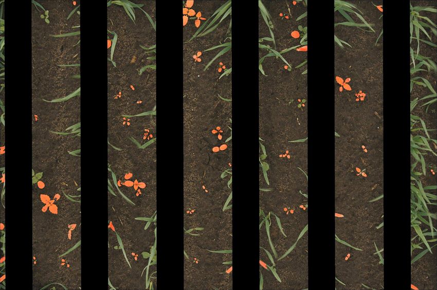
Spatial prediction of weed intensities   5

Fig. 2. Illustration of the image processing algorithm. Top: raw colour image. Middle: detection of
rows by the Hough transform. Bottom: weeds detected.
6                    G. Guillot et al.

3.           Modelling

Exact weed counts are observed at a set of sites S = (s1 , ..., sns ) and denoted by cS =
(c(s1 ), ..., c(sns )), image estimates are given at a set of sites T = (t1 , ..., tnt ) and denoted by
iT = (i(t1 ), ..., i(tnt )). We also denote by U = (u1 , ..., unu ) the set of sites at which spatial
prediction of the weed field c is sought. In our data set, the sets S and T are identical,
but we consider the case (highly relevant in practice) where the two sets do not necessarily
coincide.

3.1. Model for exact count
We consider here two models where the spatial variations are essentially captured by a
Gaussian random field.
                      5000
                      4000
                      3000
     Semi−variance

                      2000
                      1000
                      0

                             0           100        200           300               400

                                               Spatial lag (m)

Fig. 3. Empirical variograms of the exact count data c(s) for various binnings of the spatial lag, and
exponential model (dashed line) with scale parameter equal to 50 m.

3.1.1. Transformed Gaussian random field model
A first simple model accounting for spatial auto-correlation and non-Gaussian marginal
distribution is the transformed Gaussian random field model (TGRF). This model assumes
that there is a zero mean, unit variance Gaussian random field y(s), s ∈ R2 and a function ψ :
R −→ R such that c(s) = ψ(y(s)). This assumption is common in geostatistics (De Oliveira
et al., 1997; Chilès and Delfiner, 1999; Diggle et al., 2003) and sometimes for data on grids
Spatial prediction of weed intensities 7
Image index
Weed exact count
35
25
200
30
25
20
150
20
Frequency
Frequency
15
i
15
100
10
10
50
5
5
0
0
0
0 50 100 150 200 250 300 0 50 100 150 200 250 300 0 50 100 150 200 250 300
c c i
Fig. 4. From left to right: Histogram of exact weed counts, pair plot of image estimates vs. exact
counts, histogram of images estimates.
(Allcroft and Glasbey, 2003). It makes it possible to account for non-Gaussian marginal
distributions while keeping the parsimony and flexibility of Gaussian random fields for the
modelling of spatial variations.
We assume that y has a stationary and isotropic correlation function ρ(h), with expo-
nential decay, namely
Cor[y(s), y(s + h)] = exp(−||h||/κ) (1)
for some unknown spatial correlation parameter κ.
This model is common in geostatistics. Although the spatial correlation structure is
formulated in terms of y while the empirical variogram available is that of c (Fig 3), it is
known (see e.g. De Oliveira (2003)) that for a large class of continuous transformations
ψ, the variograms of the latent Gaussian field and of the observed field are quite similar.
Hence, it is expected that the exponential model gives a good fit, at least for short to
medium distances (see Section 4.1).
It is sometimes recommended to use an extra parameter to quantify the smoothness
properties of the field, (for example, within a model of the Whittle-Matèrn family). In
addition, it would be natural to consider an anisotropic model (the dispersal process of
weed being probably much influenced by the ploughing process). The inference of three
extra parameters (a smoothing parameter, the angle and ratio for geometrical anisotropy)
adds no difficulty in principle. But it can be expected that it would not improve the results
in terms of inference (in particular with the use of a data set with few exact counts), while
it would increase the computational burden. Hence we choose to keep a reasonably simple
one-parameter model for the correlation function.
3.1.2. Approximate transformed Gaussian Cox Process
The previous model places a continuous distribution on c while it is a discrete variable by
nature. A simple way to avoid this inconsistency is to assume that the previous transformed
Gaussian field defines an intensity field and that conditionally on w = ψ(y), c(s) has an
independent Poisson(w(s)) distribution. This turns out to be an approximate Cox process
with transformed Gaussian intensity and a special case of a spatial generalised linear model.
We refer to this model as to TGCP in the sequel (disregarding the approximation in the
terminology). This second approach is an example of the general modelling framework8 G. Guillot et al.
proposed by Diggle et al. (1998) and is also similar to that taken by Christensen and
Waagepetersen (2002) where the weed counts are assumed to arise from a spatial generalised
linear mixed model with a Gaussian random field as random effect, while covariates are used
to model a deterministic trend of the intensity.
We note here that under this model with Poisson regression relating c and w, we have
Cov[c(s), c(s + h)] = Cov[w(s), w(s + h)] for h > 0 (2)
and
V ar[c(s)] = E[w(s)] + V ar[w(s)] (3)
implying a discontinuity of the covariance function at 0 (a property known as nugget effect
in geostatistics). The jump at 0 is given by the mean of the intensity field E[w], so that
this parameter controls jointly two very different aspects of the model.
Regarding ψ, we considered functions such that ψ(y) has Gamma or log-normal marginal
distribution. We denote by µ and σ 2 the stationary mean and variance of ψ(y). The choice
of the marginal distribution will be discussed later, together with a comparison between the
TGCP and TGRF models.
3.2. Modelling the relationship between exact counts and image estimates
In order to capture the relationship between the two variables and the observed hetero-
scedasticity, we assume a Poisson regression model for the image estimate
i(s)|c ∼ Poisson(γc(s)δ ) (4)
where γ and δ are parameters to account for a slight departure from linearity as can be
seen in Fig. 4.
3.3. Prior distributions
The vector of unknown parameters is θ = (κ, µ, σ, γ, δ). All parameters take their value on
[0, ∞). We assume proper Gamma priors for all of them. Each such distribution has shape
and rate parameters a. and b. (where . is κ, µ, σ, γ or δ). We assume a priori independence
of the components of the vector of parameters, namely:
π(θ) = π(µ)π(σ)π(κ)π(γ)π(δ)
∝ µaµ −1 e−µbµ × σ aσ −1 e−σbσ × κaκ −1 e−κbκ × γ aγ −1 e−γbγ × δ aδ −1 e−δbδ . (5)
Having no previous information on what sensible values for the parameters θ should be,
we chose the parameters a. and b. in such a way that a. /b2. is large compared to a. /b. (flat
priors). We used moment estimates as an expedient to set the values of a. /b. , an approach
common in practice, see e.g. (Eidsvik et al., 2006). The parameters aκ and bκ were chosen to
have a mean of 80 m corresponding to a rough empirical estimate from Fig.3. We chose aµ ,
bµ , aσ and bσ so that E[µ] and E[σ] comply with the moment estimate of µ and σ, ignoring
the spatial correlation in the weed counts. Further, aγ , bγ , aδ and bδ were chosen so as to
have E[γ] = E[δ] = 1. Each such constraint gives an equation for each pair of parameters
(a. , b. ), a second equation being obtained by setting the variance of the parameter to an
arbitrary large value. Note also that the prior on κ is actually discretized on a fine regular
grid and truncated at an upper value κmax . We checked that the choice of the ratio a. /b.Spatial prediction of weed intensities 9 does not affect the result of the inference for a broad range of values. Further discussion on the choice of prior for such spatial models can be found in Berger et al. (2001) and Diggle et al. (2003). 3.4. Inference and prediction We perform jointly inference on the parameter vector θ and prediction of the vector of weed values cU . This is achieved through simulation of the joint distribution π(θ, cU |cS , iT ). However, in the two models considered, inference and prediction are greatly simplified by the use of model structure and the introduction of auxiliary variables. Instead of making prediction of c at sites U only, we also make prediction of c at sites T \ S. For the TGCP model, we also introduce the latent variable w which we sample at all the sites in S ∪ T ∪ U. Then the algorithm we use involves different updates of either Metropolis-Hastings or Gibbs type, performed in a deterministic order as described in the appendix. It is known that in such hierarchical models, see e.g. Diggle et al. (2003) for an explicit example, even under proper prior/likelihood models with finite moments, the posterior or the predictive distributions may not have finite first order moments. Thus we use the median of the simulated sample for inference and prediction. 4. Implementation on real data 4.1. Bjertorp data set: inference, convergence and goodness-of-fit assessment 4.1.1. Gamma versus log-normal transform We checked that the Gamma and the log-normal distribution gave similar results in terms of goodness of fit for the TGCP and the TGRF model. Hence, we assume hereafter that ψ(y) has a Gamma marginal distribution both for the TGRF and the TGCP model. The estimated values for the parameter α of the gamma distribution involved in the weed counts models are both small (α̂TGRF = 1.03 and α̂TGCP = 1.41) corresponding to a fairly high amount of transformation of the underlying Gaussian distribution. 4.1.2. Convergence assessment We implemented the previous algorithm on the Bjertorp data set for the TGRF and the TGCP models. We launched 20 independent runs with different initial conditions for the components of θ sampled from the prior. In order to detect potential convergence flaws, we computed the Gelman-Rubin statistics testing the significance of the difference between the within chain variance and the between chain variance. No convergence flaw was detected (values under the 97.5% quantile). Histograms of MCMC samples of the parameters for the two models are displayed in Fig. 5. 4.1.3. TGRF model versus TGCP model We checked the fit of the TGRF model and the TGCP model to data (within the global model including image estimate data) as follows: we plotted the average posterior variogram of weed counts and compared it to the empirical variograms (obtained for various binnings). We compared the distribution of a sample of h = L−1 κ y from the predictive distribution to the assumed normal distribution. (where Lκ Uκ is the Choleski decomposition of the
10    G. Guillot et al.

correlation matrix of y). We checked the fit between the image index values and a sample
from their predictive distribution by a pair plot and a quantile-quantile plot.
    This check is not rooted in a formal statistical testing (see e.g. (Waagepetersen, 2006) for
a more formal approach) but it suggests that the TGCP and TGRF models give a similar fit
regarding image index data. In contrast, regarding the weed counts, the TGRF model gives
a betters fit than the TGCP model (see fitted variogram bottom-right panel in Figure 6 and
7). This relatively poor fit of the variogram under the TGCP model might be explained
by a bad specification of the behavior of the variogram near 0. Indeed, the TGCP model
assumes a nugget effect whereas such nugget effect seems to be absent from the emprirical
variogram whatever the binning considered. The over-estimation of the scale parameter
might be a consequence of the need to reconcile the non-smooth variations induced by the
nugget effect with the rather smooth variations observed on weed conts.
Spatial prediction of weed intensities 11
TGCP TGRF
0.030
0.020
Density
Density
0.015
0.000
0.000
50 100 150 200 50 100 150 200
µ µ
average=67.7 average=80.5
0.000 0.015 0.030
0.04
Density
Density
0.02
0.00
40 50 60 70 80 90 100 40 60 80 100 120 140 160
σ σ
average=66.6 average=67.7
0.0 0.4 0.8 1.2
1.2
Density
Density
0.6
0.0
1.5 2.0 2.5 3.0 2.0 2.5 3.0 3.5 4.0
γ γ
average=2.01 average=2.74
12
15
Density
Density
10
8
4
5
0
0
0.70 0.75 0.80 0.85 0.90 0.70 0.75 0.80
δ δ
average=0.81 average=0.75
0.030
0.008
Density
Density
0.015
0.000
0.000
50 100 150 200 50 100 150 200
κ κ
average=89.3 average=46.5
Fig. 5. Posterior distribution of the parameters for a random sub-sample of the Bjertorp data set with
30 exact counts and 100 images.12 G. Guillot et al.
200
200
150
150
100
100
i*
i*
50
50
0
0
−50
−50
0 50 100 150 200 0 50 100 150 200
i i
Image index: pair plot of data vs a simulation Image index: qqplot of data vs a simulation
5000
2
4000
1
Sample Quantiles
Semi−variance
3000
0
2000
−1
1000
−2
0
−2 −1 0 1 2 0 20 40 60 80 100
h Spatial lag
Transformed Gaussian values h: qqplot for a simulation Empirical and theoretical variograms
Fig. 6. Goodness of fit plots for the TGCP model. Top left: pair plot of a sample of the predictive
distribution of i against data. Top right: quantile-quantile plot of a sample of the predictive distribution
of i against data. Bottom Left: qq-norm plot of a sample h = L−1 κ y from the predictive distribution.
Bottom right: average posterior variogram of weed counts (dash line) and empirical variograms for
various binnings.Spatial prediction of weed intensities 13
250
200
200
150
150
100
i*
i*
100
50
50
0
0
−50
0 50 100 150 200 0 50 100 150 200
i i
Image index: pair plot of data vs a simulation Image index: qqplot of data vs a simulation
5000
2
4000
1
Sample Quantiles
Semi−variance
3000
0
2000
−1
1000
−2
0
−3
−2 −1 0 1 2 0 20 40 60 80 100
Theoretical Quantiles Spatial lag
Transformed Gaussian values h: qqplot for a simulation Empirical and theoretical variograms
Fig. 7. Goodness of fit plots for the TGRF model. Top left: pair plot of a sample of the predictive
distribution of i against data. Top right: quantile-quantile plot of a sample of the predictive distribution
of i against data. Bottom Left: qq-norm plot of a sample h = L−1 κ y from the predictive distribution.
Bottom right: average posterior variogram of weed counts (dash line) and empirical variograms for
various binnings.14 G. Guillot et al.
Table 1. Mean square prediction error for subsamples of the Bjertorp data set.
Numbers in italic are MSE obtained when parameters estimated off-line are
plugged into the predictor.
Spatial sampling design TGCP TGRF (Co-)Kriging
99 counts, no image 2710 (2510) 2417 (2404) 2373
30 counts, no image 3409 (3255) 2932 (2862) 2878
10 counts, no image 5522 (4439) 3831 (3561) 3743
30 counts, 99 images 2426 2211 1998
10 counts, 99 images 4340 3240 2358
4.2. Assessment of prediction accuracy
4.2.1. Setting for the TGCP and TGRF models
We compared the TGCP model and the TGRF model in terms of accuracy of prediction of
weed counts on various sub-samples of the Bjertorp data set. We considered random sub-
samples with various numbers of exact count and image estimate sites, namely: 99/0,30/0,
10/0, 30/99 and 10/99. We considered 250 sub-samples for each case, except for the combi-
nation 99/0 where there are only 100 subsamples. Prediction was carried out for the left-out
sites (1, 30 or 70 sites) with the TGCP model and the TGRF model. Prediction was car-
ried out in Full-Bayes mode (parameters considered as unknown) but to assess the effect
of uncertainty about parameters, we also performed prediction with plugged-in parameters
from an off-line estimation.
4.2.2. Setting for kriging and co-kriging
We also implemented a linear spatial predictor (kriging or co-kriging). The variant used was
ordinary kriging. It assumes stationarity of mean and variance but accounts for unknown
mean. It was performed following the usual practice in Geostatistics (Chilès and Delfiner,
1999) consisting in using plugged-in parameters. We assumed an exponential covariance
function for the exact counts. For combinations of data using image estimates, we imple-
mented co-kriging with a linear co-regionalization model (Wackernagel, 1995). This was
implemented with the R package RandomFields (Schlather, 2006). Note that we also tried
kriging on the log transformed and cubic transformed data (and back-transform), a tech-
nique introducing a bias in the prediction but potentially reducing the MSE. It appeared
that the MSE was actually slightly larger than the one obtained with plain kriging. Hence
we do not report numerical results for that. The results in terms of mean square prediction
error (MSE) are reported in Table 1.
5. Discussion
5.1. Use of image-derived estimates
The first conclusion of this study is that using image estimates clearly improves the ac-
curacy of predictions as compared to those obtained with exact counts only. We assumed
throughout this study that some of the image data were collected at the same sites as exact
count data. All our computations
T are based on such data and it has been observed on
simulated data where S T = ∅ that the predictions were less accurate than those where
S ⊂ T in the TGRF and TGCP models, in particular because of poor estimates of the
parameters γ and δ in the Poisson regression. However the requirement that S ⊂ T isSpatial prediction of weed intensities 15
not very constraining in practice and this should not be considered as a drawback of our
study. We also note that the Poisson regression model linking images and counts assumes
the following relationship:
V ar[i] = γE[cδ ] + γ 2 V ar[cδ ] (6)
In particular, for γ and δ close to 1, we have V ar[i] ≈ E[c]+V ar[c] implying V ar[i] > V ar[c].
In the present dataset, the empirical variances of i and c rank in the opposite way which
suggests that the manual counting process involves some kind of smoothing. Our model
is therefore not perfect and perhaps a bit pessimistic and further improvement could be
probably obtained with a model enforcing a tighter relationship between i and c.
5.2. Prediction under complex models with small data sets
The second result of our analysis is that for sample sizes considered (within a range from
small to moderate), the simple models (kriging and TGRF) give more accurate prediction
than the most complex (and potentially more realistic) TGCP model. The difference ob-
served between kriging and TGRF on one hand and TGCP on the other hand is limited
when many data points are available and increases when the size of the data set decreases.
The largest difference is observed with a small number of exact counts, where kriging and
TGRF still perform well while TGCP brings large prediction errors. Figure 5 (bottom
panels) reveals that the posterior distribution of the scale parameter κ is flatter for the
TGCP model than for TGRF, giving a non-negligible weight to large values of κ. This
complies well with the modelling assumptions. Indeed, under the TGRF model, c (data)
and y (Gaussian field) are related through a deterministic relationship. In contrast, under
the TGCP model, the data do not relate directly to the Gaussian random field but only
through a conditional probability dependence hence the increased difficulty to learn from
the data and to transfer appropriately information across space.
5.3. Influence of predictor
Although the existence of first order moment in the TGCP and TGRF models is not guaran-
teed, in order to check that the results were not due to the use of the median as predictor, we
also made prediction by computing numerically the posterior mean on the simulated sam-
ples. We observed a small difference with |(c∗mean − c∗median )|/c∗median consistently below
1% both for TGRF and TGCP predictions.
5.4. Full Bayes versus plug-in prediction
Kriging prediction was performed with plug-in parameters. This contrasts with the method
we used for the Bayesian models consisting in estimating parameters and making predictions
jointly. The discrepancy between TGRF and kriging seems to be largely explained by
this fact as the use of plug-in parameters in TGRF prediction decreases MSE to a value
comparable to those obtained with kriging. This is surprising and the reasons for that are
not fully understood. We also note that inference under the TGCP model requires MCMC
computations as the intensity field w is not observed. In contrast, the off-line (MCMC-free)
inference of parameters under the TGRF model is possible as long as there is some overlap
between exact weed counts locations and image locations. Indeed, if weed counts and images
are observed at set of common sites, then γ and δ can be estimated easily. Then parameters
of the random field c can be estimated following standard geostatistical methods. This is16 G. Guillot et al.
fortunate for the TGRF model as this allows to reduce the prediction error which is often
the main goal of weed studies based on such models.
5.5. Continuous versus discontinuous covariance function
In the case of kriging, we assumed that the exact counts have an exponential covariance
function which is continuous on R. For the TGRF model, the assumption of exponential
covariance function refers on the underlying Gaussian random field y. In that case, the
covariance of the exact weed count c can not be obtained analytically, and Hermite polyno-
mials expansions are used to derive theoretical properties (Chilès and Delfiner, 1999). But
here, the continuity of the transform φ guarantees the continuity of the covariance function
of c. In contrast, under the TGCP model the covariance of the weed count is discontinuous
(see Section 3.1.2). The nugget effect (jump at 0) is equal to the mean of the intensity
field whose estimated value is 80.5. This value is small but might explain partly the lower
performance of the TGCP model for prediction.
5.6. Conclusion
The factors affecting the performances of the different approaches are (i) a better robust-
ness of kriging due to parsimony, (ii) a slight (TGRF) to moderate (TGCP) sensitivity of
Bayesian approaches to parameters uncertainty, (iii) the weak identifiability of parameters
under the TGCP model (in particular the scale parameter κ of the hidden Gaussian ran-
dom field) and (iv) the better performance for prediction of models based on a continuous
covariance function (TGRF, kriging).
In terms of practical recommendations, the conclusions to draw from our work seem
to be that with data sets similar to the one we studied in terms of sample size, spatial
design and statistical characteristics, it is good to use image estimates. Prediction should
then preferably be done with a simple model such as kriging or TGRF. We also noted that
kriging seems to be more robust than TGRF, in particular in the case where the parameters
are unknown. On the other hand, making prediction under TGRF allows to derive not only
point predictions but also probability distributions of parameters which can be useful even
when the focus is on prediction rather that on inference, e.g. for combining information of
various data sets in a meta-analysis. The interest of more sophisticated Bayesian models
such as TGCP lies potentially on the side of inference rather than on the side of prediction,
for instance if a quantification of a mean intensity is required which can be interpreted in
terms of local weed growth potential of the field.
5.7. Computer program
The program developed during this work is available from the Comprehensive R Archive
Network as an R package named WeedMap.
Acknowledgements
This work has been carried out within the project “Image analysis as a tool for site specific
weed control” funded by The Swedish Farmers Foundation for Agricultural Research (SLF).
Niklas Lorén acknowledges SLF for financial support during this work. Mats Rudemo was
supported by the Swedish Foundation for Strategic Research through the GMMC project andSpatial prediction of weed intensities 17 the Swedish Research Council through the Gothenburg Stochastic Centre. Anders Lars-Olle (SLU), Mats Söderström (Lantmännen/Sweco) and Thomas Börjesson (Lantmännen) are thanked for the preparation of Geographic Information Systems data and valuable discus- sions. We also thank our colleagues Anastassia Baxevani, Jacques de Maré, Antti Pentti- nen, Petter Mostad, Aila Särkkä and Martin Schlather for comments , in particular during the Gothenburg Stochastic Centre workshop on Spatial Modelling in 2006 in Smögen.
18      G. Guillot et al.

A.     Detail of MCMC computations

In the TGRF model, the vector of parameters and variables to be simulated is (cT \S , cU , θ)
with θ = (µ, σ, κ, γ, δ), where µ is the mean of the field ψ(y) and σ its standard deviation.
In the TGCP model, there is an extra layer and the vector of parameters and variables
to be simulated is (cT \S , cU , yS , yT \S , yU , θ). The steps involved in both algorithms are
similar and we only describe below the updates for the TGCP model.

A.1. Updating exact counts c at image data sites in T \ S
We iterate in a deterministic order single component updates cT \S . The acceptance ratio
for such a move is:

                                                   π(c∗T \S |wT \S ) π(iT \S |c∗T \S , θ)
                        a(cT \S , c∗T \S ) = 1 ∧                                                   (7)
                                                   π(cT \S |wT \S ) π(iT \S |cT \S , θ)
     where all the densities are Poisson distributions with independent components.

A.2. Updating exact counts c at prediction sites u
We iterate in a deterministic order single component updates of cU . The acceptance ratio
for such a move is:

                                                            π(c∗U |wU )
                                       a(cU , c∗U ) = 1 ∧                                          (8)
                                                            π(cU |wU )

A.3. Updating the components of the vector (yS , yT \S , yU ) of the hidden Gaussian field
     y
Denoting y∪ = (yS , yT \S , yU ), c∪ = (cS , cT \S , cU ) and Q(y∪ ) = π(cT \S , cU , y∪ , θ|cS , iT ),
we make Langevin proposals for y∪ , namely

                                     ∗              η2
                                    y∪ = y∪ +          ∂ ln Q(y∪ ) + δy∪                           (9)
                                                    2
where ∂ ln Q denotes the gradient of ln Q and δy∪ is a vector with independent Gaussian
components with zero mean and variance η 2 .
   The gradient is
                       ∂ ln Q(y∪ ) = ∂ ln π(y∪ |θ) + ∂ ln π(c∪ |θ, y∪ )            (10)
The first term is −Σy where Σ is the covariance matrix of y∪ . The second term is a vector
whose generic term is (ck /ψ(yk ) − 1)ψ 0 (yk ).
                           ∗
   The move from y∪ to y∪    is accepted with probability
                                                  ∗               ∗          ∗
                                    ∗          π(y∪ |θ) π(c∪ |θ, y∪ ) q(y∪ |y∪ )
                            a(y∪ , y∪ )=1∧                               ∗                        (11)
                                               π(y∪ |θ) π(c∪ |θ, y∪ ) q(y∪ |y∪ )
where π(y∪ |θ) is a multivariate Gaussian density, π(c∪ |θ, y∪ ) is a product of Poisson den-
sities and
                              ∗            ∗       η2
                          q(y∪  |y∪ ) = g(y∪ − y∪ − ∂ ln Q(y∪ ))                         (12)
                                                    2
where g denotes the independent centred multivariate Gaussian density.
Spatial prediction of weed intensities 19
A.4. Updating the mean µ of the intensity field w
We propose a move from µ to µ∗ by the addition of a small Gaussian increment. Note
that since we let the values of the Gaussian random field y be unchanged, the values of the
intensity field w are implicitly changed. The move is accepted with probability
π(c∪ |y∪ , θ∗ ) π(µ∗)
a(µ, µ∗ ) = 1 ∧ (13)
π(c∪ |y∪ , θ) π(µ)
A.5. Updating the variance σ 2 of the intensity field w and the scale parameter κ of the
hidden Gaussian field y.
We propose a move from σ to σ ∗ by the addition of a small Gaussian increment and
simultaneously a move from κ to κ∗ by the addition of a small uniform increment on the
discretized range of values spanned by κ. Here again, the values of the Gaussian random
field y are unchanged, the values of the intensity field w are implicitly changed. The move
is accepted with probability
π(y∪ |κ∗ ) π(c∪ |y∪ , θ∗ ) π(κ∗ ) π(σ ∗ )
a((σ, κ), (σ ∗ , κ∗ )) = 1 ∧ (14)
π(y∪ |κ) π(c∪ |y∪ , θ) π(κ) π(σ)
A.6. Updating γ and δ
We update γ and δ jointly by addition of small Gaussian increments. It would be natural
to compute the acceptance ratio accounting for all the variables available in the current
state. However, this implies evaluation of a ratio of probabilities π(i|c, θ∗ )/π(i|c, θ) where
some of the sites involved do not include image or count data, but values simulated in the
current state of the chain. We observed that this could bring some numerical instabilities,
in particular in the case where |S| is small with respect to |T |. Hence we chose to compute
the ratio disregarding the count and image values at sites T \ S (brought by the data
augmentation), and we used i and c values at sites in S ∩ T only. We found this strategy
more efficient. It avoids numerical instabilities while it preserves the convergence to the
desired target distribution of the global algorithm.
The move from (γ, δ) to (γ ∗ , δ ∗ ) is therefore accepted with probability
π(iT ∩S |cT ∩S , θ∗ )
a((γ, δ), (γ ∗ , δ ∗ )) = 1 ∧ (15)
π(iT ∩S |cT ∩S , θ)
References
Allcroft, D. and Glasbey, C. (2003) A latent Gaussian markov random-field model for spatio-
temporal rainfall disaggregation. Journal of the Royal Statistical Society, series C, 52,
487–498.
Andreasen, C., Rudemo, M. and Sevestre, S. (1997) Assessment of weed density at an early
stage by use of image processing. Weed research, 37, 5–18.
Åstrand, B. and Baerveldt, A.-J. (2002) An agricultural mobile robot with vision-based
perception for mechanical weed control. Autonomous Robots, 13, 21–35.20 G. Guillot et al. Berger, J. O., De Oliveira, V. and Sansó, B. (2001) Objective Bayesian analysis of spatially correlated data. Journal of the American Statistical Association, 96. Brivot, R. and Marchant, J. (1996) Segmentation of plants and weeds for a precision crop protection robot using infrared images. IEEE Proceedings: Vision, Image and Signal Processing, 143, 118–124. — (1998) Real-time segmentation of plants and weeds. Real-time imaging, 4, 243–253. Chilès, J. and Delfiner, P. (1999) Geostatistics. Wiley. Christensen, O. and Waagepetersen, R. (2002) Bayesian prediction of spatial count data using generalised linear mixed models. Biometrics, 58, 280–286. De Oliveira, V. (2003) A note on the correlation structure of transformed Gaussian random fields. Australian and New Zealand Journal of Statistics, 45, 353–366. De Oliveira, V., Kedem, B. and Short, D. (1997) Bayesian prediction of transformed Gaus- sian random fields. Journal of the American Statistical Association, 92, 1422–1433. Diggle, P., Moyeed, R. and Tawn, J. (1998) Model based geostatistics. Journal of the Royal Statistical Society, series C. Diggle, P., Ribeiro, P. and Christensen, O. (2003) Spatial statistics and computational methods, vol. 173 of Lecture notes in statistics, chap. An introduction to model based geostatistics, 43–86. Springer Verlag. Dille, J., Milner, M., Groetke, J., Mortensen, D. and Williams II, M. M. (2002) How good is your weed map? A comparison of spatial interpolators. Weed Science, 51, 44–55. Eidsvik, J., Martino, S. and Rue, H. (2006) Approximate Bayesian inference in spatial generalized linear mixed models. Tech. rep., Preprint series in Statistics, Norwegian University of Science and Technology. Gerhards, R. and Christensen, S. (2003) Real-time weed detection, decision making and patch spraying in maize, sugarbeet, winter wheat and winter barley. Weed research, 43, 385–392. Heisel, T., Andreasen, C. and Ersbøll, A. (1996) Annual weed distributions can be mapped with kriging. Weed Research, 36, 325–337. Heisel, T., Ersbøll, A. and Andreasen, C. (1999) Weed mapping with co-kriging using soil properties. Precision Agriculture, 1, 39 – 52. Lamb, D. W., Weedon, M. and L.J., R. (1999) Evaluating the accuracy of mapping weeds in seedling crops using airborne digital imaging: Avena spp. in seedling triticale. Weed Research, 39, 481–492. Marchant, J. (1996) Tracking of row structure in three crops using image analysis. Com- puters and Electronics in Agriculture, 15, 161–179. Marchant, J. and Brivot, R. (1995) Real-time tracking of plant rows using a Hough trans- form. Real-time imaging, 1, 363–371.
Spatial prediction of weed intensities   21

Onyango, C. and Marchant, J. (2003) Segmentation of row crop plant from weeds using
 colour and morphology. Computer and Electronics in Agriculture, 39, 141–155.
Otsu, N. (1979) A threshold selection method from grey-level histograms. IEEE transaction
  on Systems, Mans and cybernetic, 9, 62–66.
    c
Pðrez, A., López, F., Benlloch, J. and Christensen, S. (2000) Colour and shape analysis
  techniques for weed detection in cereal fields. Computer and Electronics in Agriculture,
  25, 197–212.
Rew, L. and Cousens, R. (2001) Spatial distribution of weeds in arable crops: are current
  sampling and analytical methods appropriate? Weed Research, 41, 1–18.

Rew, L., Whelan, B. and McBratney (2001) Does kriging predict weed distribution accu-
  rately enough for site-specific weed control? Weed Research, 41, 245–263.
Russ, J. (1994) The image processing handbook. Boca Raton: CRC Press, 2nd edn.
Schlather, M. (2006) RandomFields: Simulation and Analysis of Random Fields. URL
  http://www2.hsu-hh.de/schlath/index.html. R package version 1.3.29.

Soille, P. (2000) Morphological image analysis applied to crop field mapping. Image and
  Vision Computing, 18, 1025–1032.

Tillet, N., Hague, T. and Miles, S. (2001) A field assessment of potential method for weed
  and crop mapping on the basis of crop planting geometry. Computer and Electronics in
  Agriculture, 32, 229–246.
Waagepetersen, R. (2006) A simulation-based goodness-of-fit test for random effects in
 generalized linear mixed models. Scandinavian Journal of Statistics, 33, 721–73.
Wackernagel, H. (1995) Multivariate geostatistics : an introduction with applications. Berlin:
 Springer Verlag.
Woebbecke, D., Meyer, G., Bargen, K. and von Mortensen, D. (1995) Color indices for
 weed identification under various soil, residue, and lightning conditions. Trans. ASAE,
 38, 259–269.
You can also read