Speculation and price volatility in the coffee market - PROJECT DOCUMENTS Javier Aliaga Lordemann Claudio Mora-García Nanno Mulder

PROJECT DOCUMENTS

Speculation and price volatility
in the coffee market
Javier Aliaga Lordemann
Claudio Mora-García
Nanno Mulder

Thank you for your interest in
 this ECLAC publication

 ECLAC
 Publications

 Please register if you would like to receive information on our editorial
products and activities. When you register, you may specify your particular
areas of interest and you will gain access to our products in other formats.

 Register

 www.cepal.org/en/publications

 facebook.com/publicacionesdelacepal

 Publicaciones
 www.cepal.org/apps

Project Documents

Speculation and price volatility in the coffee market
 Javier Aliaga Lordemann
 Claudio Mora‐García
 Nanno Mulder

This document was prepared by Javier Aliaga Lordemann, Chief of the Regional Climate Change Program of the
Latin American and Caribbean Network of Fair Trade Small Producers and Workers (CLAC); Claudio Mora‐García,
Professor at the University of Costa Rica and Senior Researcher at INCAE Business School, in Costa Rica; and Nanno
Mulder, Chief of the International Trade Unit of the Division of Internation Trade and Integration of the Economic
Commission for Latin America and the Caribbean (ECLAC). It was prepared under the 2020 cooperation agreement
between CLAC and ECLAC. The authors are grateful for the comments received from the participants in a workshop held
on 3 November 2020 and convey thanks to the International Coffee Organization for facilitating access to its statistics.
The views expressed in this document, which has been reproduced without formal editing, are those of the authors
and do not necessarily reflect the views of the Organization.

United Nations publication
LC/TS.2021/59
Distribution: L
Copyright © United Nations, 2021
All rights reserved
Printed at United Nations, Santiago
S.21‐00282

This publication should be cited as: J. Aliaga Lordemann, C. Mora‐García and N. Mulder, “Speculation and price volatility in the
coffee market”, Project Documents, (LC/TS.2021/59), Santiago, Economic Commission for Latin America and the Caribbean
(ECLAC), 2021.

Applications for authorization to reproduce this work in whole or in part should be sent to the Economic Commission for
Latin America and the Caribbean (ECLAC), Documents and Publications Division, publicaciones.cepal@un.org. Member States and
their governmental institutions may reproduce this work without prior authorization, but are requested to mention the source and
to inform ECLAC of such reproduction.

ECLAC Speculation and price volatility in the coffee market 3

 Contents

Abstract................................................................................................................................................ 5
Introduction ......................................................................................................................................... 7
I. Determinants of price volatility (second moment) .................................................................. 9
 A. State variables ................................................................................................................... 9
 B. Economic variables ............................................................................................................ 9
 C. Market structure variables................................................................................................. 10
II. Data description and sources .................................................................................................. 13
III. Description of the time series and specifications.................................................................... 17
IV. Methodology ........................................................................................................................... 21
V. Empirical results ...................................................................................................................... 23
VI. Discussion and conclusions ..................................................................................................... 25
Bibliography ....................................................................................................................................... 27
Annex ................................................................................................................................................. 31

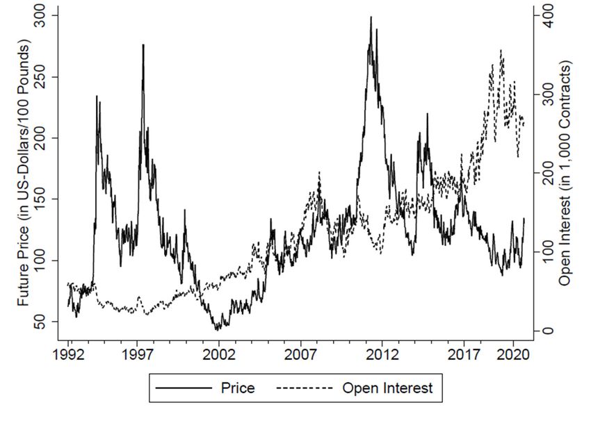
ECLAC Speculation and price volatility in the coffee market 4

Tables
Table 1 Descriptive statistics on the weekly returns on price .................................................. 19
Table 2 Results of the baseline generalized autoregressive conditional heteroskedasticity
 GARCH(1,1) model on US C contract spot and futures prices ..................................... 23
Table 3 Results of the baseline GARCH(1,1) model of volatility on spot prices
 by type of position held by speculators ......................................................................24
Table 4 Results of the baseline GARCH(1,1) model of volatility on ICO composite prices .......24
Table A1 Results of the GARCH(1,1) model of volatility on spot prices, by type
 of position held by speculators (includes all coefficients) ........................................... 32
Table A2 Results of the baseline GARCH(1,1) model of volatility on ICO composite prices ....... 33

Figures
Figure 1 Prices and ope interest in the US coffee C.................................................................. 14
Figure 2 Shares of open interest by type of commodity trader .................................................. 15
Figure 3 Weekly returns on coffee prices ................................................................................. 17
Figure 4 Autocorrelation and partial autocorrelation functions for weekly
 coffee price returns.................................................................................................... 18

Box
Box 1 Terminology: hedgers, speculators, open interest and volume .................................. 11

ECLAC Speculation and price volatility in the coffee market 5

 Abstract

This study looks into the determinants of green coffee prices’ conditional volatility in three different
markets (spot, futures and physical). For this purpose, a generalized autoregressive conditional
heteroskedasticity (GARCH) model is used. It includes weekly data on prices and control variables for
state, economic, and market structure. Conditional volatility follows a GARCH(1,1) process. Moreover,
speculation within futures markets decreases conditional volatility in all three prices.

ECLAC Speculation and price volatility in the coffee market 7

 Introduction

There is extensive literature on the determinants of spot and futures’ price volatility for several
agricultural commodities, excluding coffee. In several developing countries, many families depend
financially on green coffee farming. However, significant swings and drops in its prices have increased
poverty, considering that most farmers are smallholders (ICO, 2019). Consequently, it is crucial to study
what factors affect price volatility. Agricultural commodities have two characteristics that explain the
importance of studying volatility in spot and futures prices. On the one hand, its prices display persistent
volatility (Vivian and Wohar, 2012; Ghoshray, 2013; Karali and Power, 2013; Dawson, 2015). On the other
hand, its supply and demand have a low price elasticity. This means that relatively small production or
consumption changes induce rather significant price shifts (Tomek and Kaiser, 2014).
 In this paper, we study the determinants of price volatility in the coffee market. In particular, we
analyze the conditional volatility of three types of prices that reflect different market characteristics.
These are a) weekly spot (cash), b) futures prices of the US C Coffee contracts traded at the
Intercontinental Exchange (ICE), and c) weekly indicator prices for Arabica coffee on the physical market
collected by the International Coffee Organization (ICO). The latter are green coffee quotations in
physical markets for prompt shipment. We use a generalized autoregressive conditional
heteroskedasticity (GARCH) model to analyze price volatility, assuming a generalized error distribution
(GED). We examine the role of different types of variables related to states, the economy, and market
structure, including speculation.
 The effect of speculation on volatility has been studied for many years. Its impact ranges from
positive to negative. We measure speculation in several ways and trace its impact on different markets
and different supply chain levels. We found that a simple GARCH(1,1) process explains the conditional
volatility of the analyzed prices, i.e. a one‐period autoregressive and moving average process. We also
discovered that speculation in futures markets reduces conditional price volatility in both the spot and
futures markets and physical markets.
 This document is structured as follows. Section I reports on the main determinants of price
volatility pointed out by the literature. Section II describes the data and its sources. Section III analyzes

ECLAC Speculation and price volatility in the coffee market 8

the stationarity of the time series and the necessary transformations to comply with this condition.
Section IV describes the methodology used to analyze the data and study the relationship between
volatility and its determinants. Section V presents the outcomes. Finally, section VI puts these results in
the context of recent developments in the coffee industry and provides conclusions.

ECLAC Speculation and price volatility in the coffee market 9

 I. Determinants of price volatility (second moment)

Futures or spot price volatility for agricultural commodities has been attributed to several factors. We
mostly focus on the former but also look into the latter towards the end.1 These factors or variables can
be classified into different groups: state variables, economic variables and market structure variables.
Each is reviewed below.

 A. State variables
Early studies on the volatility of futures prices focused on the time‐to‐maturity impact. This is also
referred to as the Samuelson (1965) effect, showing that price variance increases approaching a
contract’s maturity. Other studies, in contrast, argued that the resolution of uncertainty about
underlying supply and demand “state variables” coincides with time passing (Anderson and Danthine,
1983). Moreover, Anderson (1985) and Brorsen (1989) find that seasonality drives the volatility of daily
price changes. For example, price volatility in grain markets rises in the Spring, peaks in July or August,
and falls towards the end of the year. Milonas (1986) argues that other information that influences
volatility is correlated with time‐to‐maturity.

 B. Economic variables
The second wave of studies on the volatility of futures prices examined underlying supply and demand
factors. These include inventory levels (Thurman, 1988; Williams and Wright, 1991), stocks‐to‐use and
prices‐to‐loans ratios (Kenyon et al., 1987), and price levels (Glauber and Heifner, 1986; Kenyon et al.,
1987; Streeter and Tomek, 1992). This analysis led several papers to include economic variables as
controls. For example, Kenyon et al. (1987) monitored seasonal dummies, price level, production level,
a lagged volatility effect, a ratio of the futures price to the loan rate, and a year effect. Glauber and
Heifner (1986); Kenyon et al. (1987); Streeter and Tomek (1992), and Goodwin and Schnepf (2000) find

1
 For references on this topic, see Streeter and Tomek (1992), Goodwin and Schnepf (2000) and da Silveira et al. (2017).

ECLAC Speculation and price volatility in the coffee market 10

that higher prices tend to be associated with higher levels of price variability. Also, agricultural
commodities’ price variability depends on weather conditions (e.g. temperature and rainfall) and other
stochastic elements (Hennessy and Wahl, 1996).

 C. Market structure variables
The third wave of studies includes market structure variables, such as scalping activity, market
concentration, speculation, and trading volumes. Scalping activities should reduce bid‐ask spreads, and
thus lower price variability.2 However, Brorsen (1989) argued that scalping might allow prices to adjust
to information more quickly and increase price variability. Peck (1981) found that scalping had a positive
effect on volatility. Market concentration may also affect price variability (Streeter and Tomek, 1992),
reflecting the presence of prominent positions relative to total open interest, regardless of whether
hedgers or speculators hold them. Goodwin and Schnepf (2000) pointed out that large traders’ actions
may reduce liquidity or cause significant price adjustments and therefore increase price volatility.
 The evidence on the impact of speculation on price volatility is conflicting. On the one hand, Ward
(1974), Peck (1981), Brorsen and Irwin (1987), and Irwin and Yoshimaru (1999) found that speculation reduces
volatility. On the other hand, Cornell (1981), Chang, Pinegar and Schachter (1997) and Daigler and Wiley
(1999) confirm the opposite.3 Cornell (1981) found a positive relationship between the level of volatility and
changes in daily volume. Daigler and Wiley (1999) found that the general public drives the positive volatility‐
volume relationship. The public has imprecise information, is uninformed, and cannot differentiate liquidity
demand from fundamental value change. Interestingly, Chang, Pinegar, and Schachter (1997) highlighted a
positive effect of large traders on futures daily volatility.4
 In contrast to previous models that included only one group of variables, Streeter and Tomek
(1992) developed a more comprehensive model considering all three groups’ variables. They included
state variables (time‐to‐maturity, seasonality, and price levels), economic variables (total annual supply,
monthly disappearance, and mill stocks), and market structure variables (scalping, speculation, and
market concentration). They found that speculation reduces price variance more than hedging, whereas
scalping has the opposite effect.
 The 2008 financial crisis triggered new literature on the impact of the “financialization” process
of the commodity markets on price volatility, showing mixed results (Aulerich, Irwin and Garcia, 2014).5
On the one hand, Bryant, Bessler and Haigh (2006), Haigh, Hranaiova and Overdahl (2007), and Brunetti,
Büyükşahin and Harris (2016) confirm that speculators do not influence the volatility of futures prices.
Aulerich, Irwin and Garcia (2014) found that commodity index traders (CITs) positions did not cause the
massive bubbles in agricultural futures prices. Brunetti, Büyükşahin and Harris (2016) found little
evidence that speculators destabilize financial markets and discovered that swap dealer activity is
unrelated to contemporaneous volatility. Moreover, Bohl, Javed and Stephan (2013) did not find
evidence that conditional price volatility has been affected by expected and unexpected open interest
of CITs. Sanders and Irwin (2010) also found little evidence that index funds impact commodity futures
returns. On the other hand, Irwin and Holt (2004), Du, Yu and Hayes (2011) and McPhail, Du and

2
 “Scalping” refers to traders entering and exiting the market often without having open positions at the end of the closing day. A
 standard measure of scalping is the ratio of volume to open interest.
3
 For a survey on the relation between price changes and trading volume in financial markets in general see Karpoff (1987).
4
 Bessembinder and Seguin (1993) distinguish between expected and unexpected aggregate trading volumes, while Yang, Balyeat
 and Leatham (2005) consider the unexpected overall volume.
5
 The financialization process refers to the determination of commodity prices not only by its supply and demand, but also by financial
 factors and investors’ behavior in derivative markets (Creti, Joëts and Mignon, 2013).

ECLAC Speculation and price volatility in the coffee market 11

Muhammad (2012) found a positive relationship. Beckmann and Czudaj (2014) also found evidence in
favor of an existing short‐run volatility transmission process in agricultural futures markets.6

 Box 1
 Terminology: hedgers, speculators, open interest and volume

 According to the CFTC glossary, a hedger is “a trader who enters into positions in a futures market opposite to
 positions held in the cash market to minimize the risk of financial loss from an adverse price change; or someone who
 purchases or sells futures as a temporary substitute for a cash transaction that will occur later.” A speculator is “a
 trader who does not hedge, but who trades with the objective of achieving profits through the successful anticipation
 of price movements.” A hedger uses futures markets to manage and offset risk, while a speculator assumes market
 risk for profit.
 Open interest, also called open contracts or open commitments, is the total number of futures contracts (long or
 short) held by market participants at the end of the day. This is a flow concept.
 Volume counts the number of traded contracts. This is a stock concept.

 Source: the CFTC glossary, see [online] https://www.cftc.gov/LearnAndProtect/AdvisoriesAndArticles/CFTCGlossary/index.htm.

 More generally, Algieri (2016) argues that speculation is beneficial, increasing liquidity and
commercial entities’ ability to transfer the risk of price changes and finance storage. However, excessive
speculation may cause price deviations from supply and demand fundamentals. As excessive
speculation distorts real market price dynamics, it overcomes the need to satisfy net hedging
transactions and market liquidity.
 Other studies on the relationship between futures markets and the volatility of spot prices found
mixed results. Bohl and Stephan (2013) did not find evidence that speculation in futures markets of raw
materials increased the volatility of spot prices. However, Algieri (2016) discovered speculation in the
futures markets does lead to higher volatility of spot prices.

6
 According to the Commodity Futures Trading Commission (CFTC), a commodity index fund is “an investment fund that enters into
 futures or commodity swap positions for the purpose of replicating the return of an index of commodity prices or commodity futures
 prices.” In addition, a commodity index trader (CIT) can be described as “an entity that conducts futures trades on behalf of a
 commodity index fund or to hedge commodity index swap positions.” Two well‐diversified and transparent benchmark indicators
 are the Standard and Poor’s‐Goldman Sachs (S&P‐GSCI) and the Dow Jones‐UBS Commodity Index (DJ‐UBSCI). The activities of
 CITs are also referred as the equitization or securitization of commodity futures (Bohl and Stephan, 2013).

ECLAC Speculation and price volatility in the coffee market 13

 II. Data description and sources

This section explains the sources and features of our time series. We used weekly spot and futures prices
on the US ‘C’ Contract for Arabica Coffee traded at the InterContinental Exchange (ICE) market from
January 1990 to September 2020. This is a continuous contract for Arabica coffee.7 We complemented
this data with weekly averages of ICO indicator prices for Arabica coffee. Three groups make up this
indicator price: Brazilian Naturals, Colombian Milds, and Other Milds. ICO indicator prices are a
weighted average of daily prices of green coffee on the physical markets in the United States, France,
and Germany. Prices are for prompt shipment (within 30 calendar days —instead of immediate
shipment) and sales from the origin; quotations come from at least five traders and brokers. Therefore,
ICO’s prices are essentially spot prices. ICO indicator prices and the Coffee C Contract traded at ICE are
correlated as traders and brokers often trade green coffee as Coffee C Contract including a margin.
 Weekly data on open interest for each Tuesday is taken from Commitments of Traders (COT)
reports issued by the Commodity Futures Trading Commission (CFTC). The COT disaggregate open
interest by different market participants and outline whether they are holding long or short positions. The
COT splits the number of long and short positions of major futures markets and options into commercial
and non‐commercial traders (i.e., hedgers and speculators) and non‐reportables (i.e. small traders). A
hedger uses futures markets to manage and offset risk, while a speculator assumes market risk for profit
(see Box 1 below). In this respect, only data on futures markets was considered. The sample period started
in October, 1992 when the weekly COT report became available.
 We also use monthly inventory data for Arabica Coffee from the ICE (i.e., historical end‐of‐month
certified Coffee C stocks by port held by ICE Futures US Licensed Warehouses measured in total bags).
Inventories act as buffers that absorb shocks to demand and supply affecting spot prices (Kim, 2015, pg. 701).

7
 The market and exchange names of the Coffee C contract changed over time. Until August 2007, it was the Coffee, Sugar and Cocoa
 Exchange. From September 2007 to December 2019, it was the New York Board of Trade. From January 2020 onwards, it is ICE
 Futures United States. Futures prices are taken from https: //www.investing.com/commodities/us‐coffee‐c, which are for the
 contract with the nearest delivery month. Cash/spot prices are from https://www.barchart.com/futures/quotes/KCY00/interactive‐
 chart.

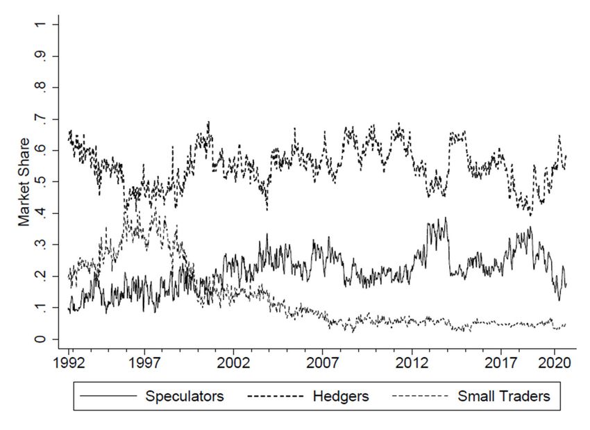
ECLAC Speculation and price volatility in the coffee market 14

 We also included macroeconomic indicators to capture the effect of supply and demand shocks.
We used quarterly gross domestic product (GDP, Billions of Dollars, Quarterly, Seasonally Adjusted)
growth rate and monthly Producer Price Index for All Commodities (Not Seasonally Adjusted), and the
Industrial Production Index (Seasonally Adjusted) growth rates. These variables were taken from the
Federal Reserve Economic Data (FRED) of the Federal Reserve Bank of St. Louis’ website.
 Figure 1 shows weekly open interest and prices for the US Coffee C contract. Prices increased from
a minimum of US$42.6 on November 25, 2001, to a maximum of US$164.6 on February 24, 2008.
Afterward, they dropped again to a minimum of US$108.4 on December 21, 2008. Subsequently, prices
increased again, reaching a historical maximum of US$299.35 in April 2011. Other commodities —such as
corn, soybeans, sugar, and wheat — showed similar price movements.

 Figure 1
 Prices and ope interest in the US coffee C

Source: Elaboration by the authors based on the cited data sources in section 3.

 For its part, aggregate open interest (OI) in the Coffee C market has persistently increased over the
analyzed period. This trend is referred to as “financialization of the commodity market” (Aulerich, Irwin
and Garcia, 2014). Between January 2000 and March 2017, OI increased 286% for Arabica. It reached a
record high during the financial crisis but plummeted until mid‐2009. Later on, it consistently rose again.
 Figure 2 displays the shares of open interest by type of trader. These are expressed as ratios of long
plus short positions to twice the aggregate open interest. A higher share of short or long positions held by
non‐commercial traders reflects increased speculation. From October 1992 to November 2013, the
speculators’ share increased from 10% to almost 40%. In the same period, the hedgers’ share fluctuated
between 50% and 70%. Small traders lost more than half of their participation. Other agricultural and
energy commodities show similar trends.

ECLAC Speculation and price volatility in the coffee market 15

 Figure 2
 Shares of open interest by type of commodity trader
 (Decimals)

Source: Elaboration by the authors based on the cited data sources in section 3.

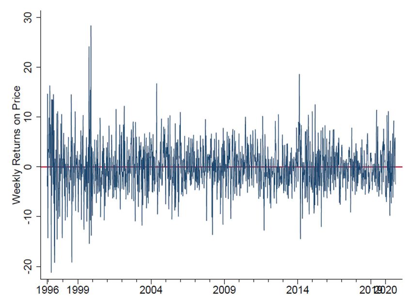
ECLAC Speculation and price volatility in the coffee market 17

 III. Description of the time series and specifications

Figure 1 showed that the time series for prices and open interest are autocorrelated. The price series has
no clear linear trend except for periods of large swings or instability followed by a more stable period.
This feature is known as a volatility persistence. The open interest series shows a deterministic trend.
As a result, we modified prices in levels and calculated price returns —defined as the weekly change on
the natural logarithm of the price ( − ln ). This is a common step made in the literature
dealing with agricultural commodity prices. The main feature of is that it is more similar to a stationary
process than , see figure 3.
 Figure 3
 Weekly returns on coffee prices

Source: Elaboration by the authors based on the cited data sources in section 3.

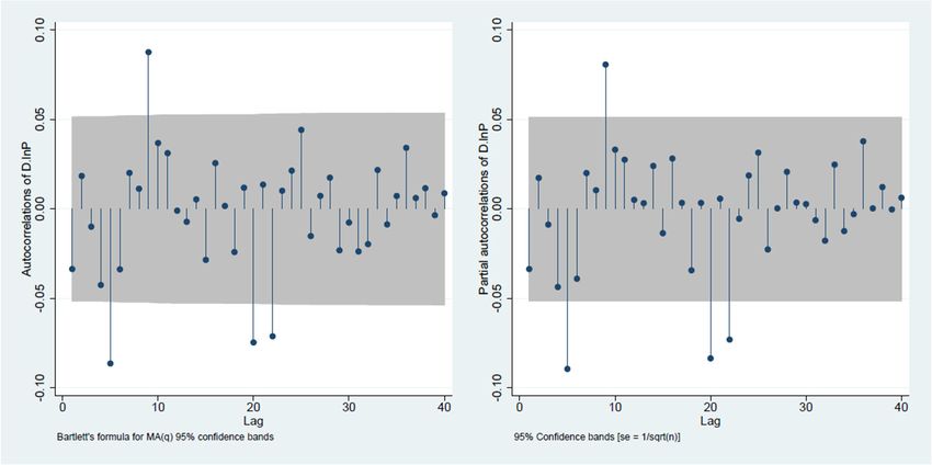
ECLAC Speculation and price volatility in the coffee market 18

 Next, we analyzed the stationarity of . The joint tests of autocorrelation were inconclusive.
Portmanteau Q‐statistic from Ljung and Box (1978) rejects the null of no white noise (Q = 62.0405 and
p = 0.0143), while the periodogram‐based test does not reject the null (B = 0.9743 and p = 0.2986).
However, the autocorrelation and partial autocorrelation functions of the series rt, shown in Figure 4,
are statistically different from zero at lags 5, 9, 20 and 22.
 Figure 4
 Autocorrelation and partial autocorrelation functions for weekly coffee price returns

Source: Elaboration by the authors based on the cited data sources in section 3.

 The Dickey‐Fuller test under different specifications (without drift or trend, with drift, with trend)
rejects the existence of a unit root at the 1% level. The Augmented Dickey‐Fuller test —including
different lags, up to the 10th lag, the DF‐GSL unit‐root test, and the Phillips‐Perron non‐parametric
test—, reject the existence of a unit root test at the 1% level. Finally, the Kwiatkowski et al. (1992) test
does not contradict the existence of level stationarity at the 1% level.
 We tried fitting different ARMA models for , but based on simplicity, the Akaike and Schwarz
information criteria, and the previous results, the preferred model is a simple model, i.e.
the fluctuation of around the long‐term means price return is given by a white noise term.
 We also tested the presence of autocorrelation in the errors . The Durbin‐Watson d statistic has
a value of 2.07, and the result of the Breusch‐Godfrey LM test depends on the number of lags selected
(for one lag, we cannot reject the null of no serial correlation, while with five lags, based on simplicity,
the Akaike and Schwarz information criterions, we can reject at the 1% level).
 Finally, the LM test for autoregressive conditional heteroskedasticity (ARCH) rejects no ARCH
effects at the 1% level.
 Table 1 shows descriptive statistics on the weekly price returns. These returns are skewed to the
right, and show excess kurtosis (i.e. leptokurtosis). As a result, the Jarque‐Bera test of normality is
rejected. We assessed whether the errors . followed or not a normal distribution. The Shapiro‐Wilk
and Shapiro‐Francia tests, and the Doornik‐Hansen test reject the hypothesis that the errors are
normally distributed. This is important for GARCH estimation by ML.

ECLAC Speculation and price volatility in the coffee market 19

 Table 1
 Descriptive statistics on the weekly returns on price
 Standard
 Mean Maximum Minimum Skewness Kurtosis Jarque-Bera
 deviation
 (1) (2) (3) (4) (5) (6) (7)
 Coffee 0.0508 42.9134 -21.2530 5.0811 0.6245 8.1054 100.8952***

Source: Elaboration by the authors based on the cited data sources in section 3.
Notes: descriptive statistics are shown for the return distributions of ICE US Coffee C. Continuously compounded weekly returns (in percent)
are calculated as the change in logarithmic prices multiplied by 100. *** Statistical significance at the 1% level.

ECLAC Speculation and price volatility in the coffee market 21

 IV. Methodology

To quantify the relation between the coffee price volatility and speculation, we used a generalized
autoregressive conditional heteroscedasticity GARCH(1,1) model, and extended the volatility equation
by including speculative open interest.8 We also monitored the impact of aggregate trading activity by
considering both overall trading volume and open interest. Given the previous analysis, price changes
are modeled as a simple rt = c + εt model. ARCH models were introduced by Engle (1982) and then
generalized and extended by Bollerslev (1986) to the GARCH model.
 Our first model (Model 1) is as follows:
 (i) = + 
 (ii) = 
 (iii) = + + 
 where are independent and identically distributed random variables, includes a vector of
potential explanatory variables for the volatility of coffee price returns . These variables include the
weekly percentage change in: a) the aggregate futures trading volume of the Coffee C contracts
(%∆TV), b) the aggregate open interest (%∆OI), and c) futures positions held by speculators (%∆SP). All
three are measured using the Coffee C contracts to compare the results with those of Bohl and Stephan
(2013), who use a similar specification, hence = %∆ + %∆ + %∆ . The
coefficient measures the relationship between speculation and price volatility. A negative sign or a
non‐significant coefficient signals that speculators have a stabilizing to null effect on the volatility of
price returns, respectively. The coefficient α measures the ARCH term, and ϕ the GARCH term.
 However, the speculators’ position is part of the total open interest. Therefore, Bohl and Stephan’s
estimation included two variables: futures position held by speculators and aggregate open interest in the

8
 Hansen and Lunde (2005) compare over 300 volatility models and show that the GARCH(1,1) model well describes and well predicts
 the conditional variance of financial assets.

ECLAC Speculation and price volatility in the coffee market 22

conditional variance equation. This first variable is redundant as it is part of the second variable (Kim, 2015).
A second specification (Model 2) excludes total open interest and instead uses aggregate trading activity by
speculators, hedgers, and small traders. As part of our estimation, the trading volume captures the total
trading activity in the futures market. Therefore, = %∆ + %∆ + %∆ +
 %∆ , where the new variables %∆ and %∆ are the percentage change in futures positions held
by hedgers (commercial) and non‐reportable (i.e. small traders), respectively.
 In Model 3, we modified equation (1) to = + + + to include an AR(1) term in
weekly price returns and several control variables = %∆ + %∆ + %∆ where
the new variables %∆ and %∆ are the monthly percentage change in inventories and
Producer Price Index for All Commodities (as a proxy for inflation), respectively. We also changed equation
(3) to include = %∆ + %∆ + %∆ + %∆ + %∆ + %∆ +
 %∆ + %∆ + ∑ ( ) where the new variables %∆ and %∆ are the
quarterly percentage change in GDP and the monthly percentage change in the Industrial Production Index,
respectively. We also added a seasonality effect captured by the quarterly variables ( = 1 for the first
quarter and 0 otherwise, = 1 for the second quarter and 0 otherwise, = 1 for the third quarter and
0 otherwise, the fourth quarter being the omitted category).9
 Our model adds − = to both sides of the equation (3), obtaining = + +
 + , where | = 0 and | = ( ) = 2 . Most GARCH models are estimated
by maximum likelihood, assuming that is normally distributed and drawing on the Bollerslev and
Wooldridge (1992) robust covariance matrix; however, if the spreads are highly non‐normal (e.g., with
negative skewness and high kurtosis), then a generalized error distribution for may be used, which
was introduced in the GARCH literature by Nelson (1991). Given the features of our time series
highlighted in table 1, the last one is the one we used to calculate robust standard errors.10

9
 Huchet and Fam (2016) use different macroeconomic variables including the US inflation‐indexed bonds, the VIX index of the
 Chicago Board Option Exchange (CBOT) and the West Texas Intermediate (WTI) oil price.
10
 We also tried fitting the model with a Normal and a t‐distributions. For the normal distribution, the Jarque‐Bera test rejected the
 null of a normal distribution at the 1% level, while the Kolmogorov‐Smirnov test did not at the 10% level, but the Q‐Q plot displayed
 long tails. For the t‐distribution, the Kolmogorov‐Smirnov test did not reject the null of a t‐distribution, but the Q‐Q plot also
 displayed long tails.

ECLAC Speculation and price volatility in the coffee market 23

 V. Empirical results

Table 2 reports the estimation results using the GARCH(1,1) model described in equations (1) to (3),
examining the relationship between price volatility and speculation. Each row shows the respective
explanatory variable, where Resid2 corresponds to and volatility to . Column (1) shows the
results from Model 1. We do not report the coefficients from all control variables, such as the percentage
change in trading volume and aggregate open interest. The estimate for %∆ indicates that there is a
negative relationship between volatility and speculation, meaning that speculation tends to reduce
coffee price volatility. This relationship is highly statistically significant at the 1% level.
 Table 2
 Results of the baseline generalized autoregressive conditional heteroskedasticity GARCH(1,1)
 model on US C contract spot and futures prices
 Spot prices Futures prices
 Model 1 Model 2 Model 3 Model 1 Model 2 Model 3
 (1) (2) (3) (4) (5) (6)
 Resid2 0.1104* 0.1145** 0.1293*** 0.1299*** 0.1290*** 0.1503**
 Volatility 0.7537*** 0.7114** 0.3986 0.5609** 0.5569*** 0.2480
 %∆SP -0.0642*** -0.0545*** -0.0441*** -0.0440* -0.0440*** -0.0315**
 %∆H -0.0590 0.0343 -0.0741* -0.0180
 %∆NR -0.0032 -0.0090 -0.0035 -0.0096
 %∆INV 0.0043** 0.0040**
 %∆PPIACO 0.0030 -0.0279
 %∆GDP 0.0753 -0.0126
 %∆PROD -0.0624 -0.0378
 Quarterly
 NO NO YES NO NO YES
 Fixed Effects

Source: Elaboration by the authors based on the cited data sources in section 3.
Notes: The dependent variables are either the weekly returns on spot/cash prices (columns 2 to 4) or futures prices of the contract with the
nearest delivery month (columns 5 to 7). Results are estimated by maximum likelihood using a generalized error distribution (GED) and
robust standard errors. Each column shows a different model with new covariates. In model 1, the control variables are the weekly
percentage change in the aggregate futures trading volume of the Coffee C contracts (%∆TV ) and the aggregate open interest (%∆OI), at
the Coffee C contracts. Model 2 does not control for open interest but includes the percentage change in futures positions held by hedgers
(commercial) and non‐reportable (i.e. small traders). Model 3 includes an AR(1) term in weekly price returns, open interest, inventories and
inflation in the price equation, and also includes quarterly GDP and monthly industrial production in the volatility equation. Statistically
significant at * 10%, ** 5%, and *** 1% level.

ECLAC Speculation and price volatility in the coffee market 24

 Column (2) shows the results for Model 2, after controlling for the percentage change in futures
positions held by hedgers and small traders, but not controlling for open interest. The estimate for
%∆SP is similar, while hedgers and small traders have a statistically insignificant impact on volatility.
Column (3) shows the results from Model 3, i.e. monitoring an AR(1), open interest, inventories, and
inflation in the price equation, and including inventories, inflation, GDP, and industrial production. The
results are similar to the previous model, suggesting that speculation reduces volatility in coffee prices.
In sum, models (1), (2), and (3) seem to confirm that speculation tends to dampen coffee price volatility.
 To examine if the relationship between volatility and speculative activities differs with the kind of
position held by speculators, we decompose ( %∆ + %∆ + %∆ ) into a long and short
position.11 Table 3 displays only the estimated coefficients for the effect of the speculators, while Annex
Table A1 shows all the coefficients. The estimated coefficients for speculators’ long and short positions are
mostly negative or statistically insignificant. This suggests that there is no evidence that speculators’ long
and short positions accentuate volatility. These results also show that coefficients on speculative short
positions are negative, implying that volatility tends to decrease when speculators are selling.
 Table 3
 Results of the baseline GARCH(1,1) model of volatility on spot prices by type of position held by speculators
 Model 1 Model 2 Model 3
 (1) (2) (3)
 %∆ Total positions -0.0642*** -0.0545*** -0.0441***
 %∆ Long positions 0.0410** -0.0101 -0.0014
 %∆ Short positions -0.0256*** -0.0277*** -0.0316***

Source: Elaboration by the authors based on the cited data sources in section 3.
Notes: this table follows the specification in Table 2, but decomposes the effect of speculation θ1%∆SPt into long and short positions held
by speculators effect in Model 1, and changes the control variables θ1%∆SPt + θ2%∆Ht + θ3%∆NRt into θ1%∆SP_Shortt + θ2%∆H_Shortt
+ θ3%∆NR_Shortt for the short position and θ1%∆SP_Longt + θ2%∆H_Longt + θ3%∆NR_Longt for the long position, where %∆SP_Shortt
is the percentage change in the speculators holding a short position, for example, in Models 2 and 3. Statistically significant at * 10%, ** 5%,
and *** 1% level.

 We now examine conditional volatility in ICO composite prices as the dependent variable and
keep the same specifications as in Models 1‐3. For this purpose, we use a weighted average of Brazil,
Colombia and Other Milds in Table 4 that we refer to as the “Arabica category”. In Annex Table A1, we
present the full results for each individual Arabica. According to Table 4, the speculation stabilizing
effect almost doubles across the different models. The results for Colombia and Other Milds, presented
in Table 4, suggest that the speculation stabilizing effect almost doubles across the different models.
Annex Table A2 illustrates the results for each type of Arabica.
 Table 4
 Results of the baseline GARCH(1,1) model of volatility on ICO composite prices
 Arabica
 Model 1 Model 2 Model 3
 (1) (2) (3)
 Resid2 0.1119*** 0.1127*** 0.08787***
 Volatility 0.6338*** 0.6429*** 0.6627***
 %∆SP -0.1145*** 0.0894*** 0.0865***
 %∆H 0.0513 0.0490
 %∆NR 0.0021 -0.0010

Source: Elaboration by the authors based on the cited data sources in section 3.
Notes: Statistically significant at * 10%, ** 5%, *** 1% level.

11
 Specifically, θ1%∆SP_Shortt + θ2%∆H_Shortt + θ3%∆NR_Shortt for the short position and θ1%∆SP_Longt + θ2%∆H_Longt + θ3%∆NR_Longt
 for the long position, where %∆SP_Shortt is the percentage change in the speculators holding a short position, for example.

ECLAC Speculation and price volatility in the coffee market 25

 VI. Discussion and conclusions

In this paper, we used a GARCH(1,1) model to identify the determinants of the conditional volatility of
prices in the Coffee C market and ICO composite prices for Arabica coffee. Analyzing a comprehensive
set of state, economic, and market structure variables, we found that speculation tends to reduce
volatility in the coffee market. This result is similar to those of Bohl and Stephan (2013), and Kim (2015).
 As speculation stabilizes prices (both during the upward and downward trends) for coffee growers,
they can draw up and implement their investment plans with less risk. This is especially important for
commodities such as coffee, which production cycle is relatively long (around three years). Also, investments
will take place with lower expected returns compared to a scenario of higher price volatility.

ECLAC Speculation and price volatility in the coffee market 27

 Bibliography

Algieri, Bernardina (2016), “Conditional price volatility, speculation, and excessive speculation in commodity
 markets: sheep or shepherd behaviour?” International Review of Applied Economics, 30(2): 210–237.
Anderson, Ronald W. (1985), “Some determinants of the volatility of futures prices.” Journal of Futures
 Markets, 5(3): 331–348.
Anderson, Ronald W. and Jean‐Pierre Danthine (1983), “The Time Pattern of Hedging and the Volatility of
 Futures Prices.” The Review of Economic Studies, 50(2): 249.
Aulerich, Nicole M., Scott H. Irwin and Philip Garcia (2014), “Bubbles, Food Prices, and Speculation. Evidence
 from the CFTC’s Daily Large Trader Data Files.” In The Economics of Food Price Volatility, ed. Jean‐Paul
 Chavas, David Hummels and Brian D. Wright, Chapter 6. Chicago, IL:The University of Chicago Press.
Beckmann, Joscha, and Robert Czudaj (2014), “Volatility transmission in agricultural futures markets.”
 Economic Modelling, 36: 541–546.
Bessembinder, Hendrik and Paul J Seguin (1993), “Price Volatility, Trading Volume, and Market Depth:
 Evidence from Futures Markets.” The Journal of Financial and Quantitative Analysis, 28(1): 21–39.
Bohl, Martin T. and Patrick M. Stephan (2013), “Does Futures Speculation Destabilize Spot Prices? New
 Evidence for Commodity Markets.” Journal of Agricultural and Applied Economics, 45(4): 595–616.
Bohl, Martin T., Farrukh Javed and Patrick M. Stephan (2013), “Do Commodity Index Traders Destabilize
 Agricultural Futures Prices?” Applied Economics Quarterly, 59(2): 125–148.
Bollerslev, Tim (1986), “Generalized autoregressive conditional heteroskedasticity.” Journal of Econometrics,
 31(3): 307–327.
Bollerslev, Tim and Jeffrey M. Wooldridge (1992), “Quasi‐maximum likelihood estimation and inference in
 dynamic models with time‐varying covariances.” Econometric Reviews, 11(2): 143–172.
Brorsen, B Wade (1989), “Liquidity costs and scalping returns in the corn futures market.” Journal of Futures
 Markets, 9(3): 225–236.
Brorsen, B Wade and Scott H Irwin (1987), “Futures funds and price volatility.” Review of Futures Markets, 6(2):
 118–135.
Brunetti, Celso, and David Reiffen (2014), “Commodity index trading and hedging costs.” Journal of Financial
 Markets, 21: 153–180.

ECLAC Speculation and price volatility in the coffee market 28

Brunetti, Celso, Bahattin Büyükşahin and Jeffrey H. Harris (2016), “Speculators, Prices, and Market
 Volatility.” Journal of Financial and Quantitative Analysis, 51(5): 1545–1574.
Bryant, Henry L., David A. Bessler and Michael S. Haigh (2006), “Causality in futures markets.” Journal of
 Futures Markets, 26(11): 1039–1057.
Chang, Eric C., J. Michael Pinegar, and Barry Schachter (1997), “Interday variations in volume, variance and
 participation of large speculators.” Journal of Banking & Finance, 21(6): 797–810.
Cornell, Bradford (1981), “The relationship between volume and price variability in futures markets.” Journal
 of Futures Markets, 1(3): 303–316.
Creti, Anna, Marc Joëts and Valérie Mignon (2013), “On the links between stock and commodity markets’
 volatility.” Energy Economics, 37: 16–28.
Daigler, Robert T. and Marilyn K. Wiley (1999), “The impact of trader type on the futures volatility‐volume
 relation.” Journal of Finance, 54(6): 2297–2316.
da Silveira, Rodrigo Lanna Franco, Leandro dos Santos Maciel, Fabio L. Mattos and Rosangela Ballini (2017),
 “Volatility persistence and inventory effect in grain futures markets: evidence from a recursive model.”
 Revista de Administração, 52(4): 403– 418.
Dawson, P. J. (2015), “Measuring the Volatility of Wheat Futures Prices on the LIFFE.” Journal of Agricultural
 Economics, 66(1): 20–35.
Du, Xiaodong, Cindy L. Yu and Dermot J. Hayes (2011), “Speculation and volatility spillover in the crude oil
 and agricultural commodity markets: A Bayesian analysis.” Energy Economics, 33(3): 497–503.
Engle, Robert F. (1982), “Autoregressive Conditional Heteroscedasticity with Estimates of the Variance of
 United Kingdom Inflation.” Econometrica, 50(4): 987–1007.
Ghoshray, Atanu (2013), “Dynamic persistence of primary commodity prices.” American Journal of
 Agricultural Economics, 95(1): 153–164.
Glauber, Joseph W. and Richard G. Heifner (1986), “Forecasting Futures Price Variability.” Proceedings of the
 NCCC‐134 Conference on Applied Commodity Price Analysis, Forecasting, and Market Risk Management.
 St. Louis, MO.
Goodwin, Barry K. and Randy Schnepf (2000), “Determinants of endogenous price risk in corn and wheat
 futures markets.” Journal of Futures Markets, 20(8): 753–774.
Haigh, Michael S., Jana Hranaiova and James A. Overdahl (2007), “Hedge Funds, Volatility and Liquidity
 Provision in Energy Futures Markets.” The Journal of Alternative Investments, 9(4): 10–38.
Hennessy, David A., and Thomas I. Wahl (1996), “The Effects of Decision Making on Futures Price Volatility.”
 American Journal of Agricultural Economics, 78(3): 591–603.
ICO (2019), “Growing for Prosperity. Economic viability as the catalyst for a sustainable coffee sector.”
 International Coffee Organization September.
Irwin, Scott H. and Bryce Holt (2004), “The Effects of Large Hedge Funds and CTA Trading on Futures Market
 Volatility.” In Commodity Trading Advisors: Risk, Performance Analysis and Selection, ed. Greg N.
 Gregoriou, François‐Serge L’Habitant, Vassilios N. Karavas and Fabrice Rouah, 151–182. New York,
 NY: John Wiley and Sons.
Irwin, Scott H. and Satoko Yoshimaru (1999), “Managed futures, positive feedback trading, and futures price
 volatility.” Journal of Futures Markets, 19(7): 759–776.
Karali, Berna and Gabriel J. Power (2013), “Short‐ and Long‐Run Determinants of Commodity Price
 Volatility.” American Journal of Agricultural Economics, 95(3): 724–738.
Karpoff, Jonathan M. (1987), “The Relation Between Price Changes and Trading Volume: A Survey.” The
 Journal of Financial and Quantitative Analysis, 22(1): 109.
Kenyon, David, Kenneth Kling, Jim Jordan, William Seale and Nancy Mc‐Cabe (1987), “Factors affecting
 agricultural futures price variance.” Journal of Futures Markets, 7(1): 73–91.
Kim, Abby (2015), “Does Futures Speculation Destabilize Commodity Markets?” Journal of Futures Markets,
 35(8): 696–714.
Kwiatkowski, Denis, Peter C.B. Phillips, Peter Schmidt and Yongcheol Shin (1992), “Testing the null hypothesis of
 stationarity against the alternative of a unit root.” Journal of Econometrics, 54(1‐3): 159–178.
Ljung, G. M. and G. E. P. Box (1978), “On a measure of lack of fit in time series models.” Biometrika, 65(2): 297–303.

ECLAC Speculation and price volatility in the coffee market 29

McPhail, Lihong Lu, Xiaodong Du and Andrew Muhammad (2012), “Disentangling Corn Price Volatility: The Role
 of Global Demand, Speculation, and Energy.” Journal of Agricultural and Applied Economics, 44(3): 401–410.
Milonas, Nikolaos T. (1986), “Liquidity and Price Variability in Futures Markets.” Financial Review, 21(2): 211–238.
Nelson, Daniel B. (1991) “Conditional Heteroskedasticity in Asset Returns: A New Approach.” Econometrica1,
 59(2): 347–370.
Peck, Anne E. (1981), “The Adequacy of Speculation onthe Wheat, Corn, and Soybean Futures Markets.”
 Research in Domestic and International Agribusiness Management, 2: 17–29.
Samuelson (1965), “Samuelson, Paul A., Proof That Properly Anticipated Prices Fluctuate Randomly,
 Industrial Management Review, 6:2 (1965: Spring) p.41.” Management, 2.
Sanders, Dwight R. and Scott H. Irwin (2010), “A speculative bubble in commodity futures prices? Cross‐
 sectional evidence.” Agricultural Economics, 41(1): 25–32.
Streeter, Deborah H. and William G. Tomek (1992), “Variability in soybean futures prices: An integrated
 framework.” Journal of Futures Markets, 12(6): 705–728.
Thurman, Walter N. (1988), “Speculative Carryover: An Empirical Examination of the U.S. Refined Copper
 Market.” The RAND Journal of Economics, 19(3): 420.
Tomek, William G. and Harry M. Kaiser (2014), Agricultural Product Prices. . 5 ed., Cornell University Press.
Vivian, Andrew and Mark E. Wohar (2012), “Commodity volatility breaks.” Journal of International Financial
 Markets, Institutions and Money, 22(2): 395–422.
Ward, Ronald W. (1974), “Market Liquidity in the FCOJ Futures Market.” American Journal of Agricultural
 Economics, 56(1): 150–154.
Williams, Jeffrey C. and Brian D. Wright (1991), Storage and Commodity Markets. New York: Cambridge
 University Press.
Yang, Jian, R. Brian Balyeat and David J. Leatham (2005), “Futures Trading Activity and Commodity Cash
 Price Volatility.” Journal of Business Finance & Accounting, 32(1‐2): 297–323.

ECLAC Speculation and price volatility in the coffee market 31

 Annex

ECLAC
 Table A1
 Results of the GARCH(1,1) model of volatility on spot prices, by type of position held by speculators (includes all coefficients)

 (1) (2) (3) (4) (5) (6) (7) (8) (9)

 BASELINE MODEL LONG POSITIONS SHORT POSITIONS

 Model 1 Model 2 Model 3 Model 1 Model 2 Model 3 Model 1 Model 2 Model 3

 ARCH

 Resid2 0.1104** 0.1145*** 0.1293*** 0.1001*** 0.1162** 0.1190*** 0.1185*** 0.1155*** 0.0939***

 Volatility 0.7537*** 0.7114*** 0.3986 0.8203*** 0.7257** 0.6763*** 0.7342*** 0.7378*** 0.5697***

 HET
 %∆SP -0.0642*** -0.0545*** -0.0441***
 %∆H -0.0590 0.0343
 %∆NR -0.0032 -0.009
 %∆SP Long 0.0410*** -0.0101 0.0014
 %∆H Long -0.0908 -0.0601**
 %∆NR Long 0.0046 -0.0083
 %∆SP Short -0.0256*** -0.0277*** -0.0316***

 Speculation and price volatility in the coffee market
 %∆H Short -0.0172 -0.0156
 %∆NR Short -0.0138** -0.0081

 %∆OI -0.0066 -0.1112** -0.0148

 %∆VOL 0.0099*** 0.0111*** 0.0112*** 0.0102*** 0.0105** 0.0119*** 0.0095*** 0.0104*** 0.0108***
 %∆INV 0.0043** 0.0045** 0.0039**
 %∆PPIACO 0.003 -0.0137 -0.0185
 %∆GDP 0.0753 0.0465 0.0577
 %∆PROD -0.0624 -0.0408 -0.0304
 Quarterly
 Fixed Effects NO NO YES NO NO YES NO NO YES

Source: Elaboration by the authors.
Notes: Statistically significant at * 10%, ** 5%, *** 1% level.

 32

ECLAC Speculation and price volatility in the coffee market 33

 Table A2
 Results of the baseline GARCH(1,1) model of volatility on ICO composite prices

 Brazil Colombia Others
 Model 1 Model 2 Model 3 Model 4 Model 5 Model 6 Model 7 Model 8 Model 9
 (1) (2) (3) (4) (5) (6) (7) (8) (9)
 Resid2 0.1060*** 0.1067*** 0.0888*** 0.1263*** 0.1265*** 0.0914** 0.1254*** 0.1244*** 0.0870***
 Volatility 0.6780*** 0.6899*** 0.7255*** 0.6117*** 0.6198*** 0.6257*** 0.6271*** 0.6366*** 0.6536***
 %∆SP -0.1160*** -0.0882*** -0.0878*** -0.1134*** -0.0930*** -0.0895*** -0.1077*** -0.0866*** -0.0839***
 %∆H 0.0427 0.0477 0.0471 0.0426 0.0325 0.0296
 %∆NR 0.0014 -0.0026 0.0002 -0.0012 -0.0006 -0.0046

Source: Elaboration by the authors.
Note: Significant at * 10%, ** 5%, *** 1% level.

Green coffee growers, most of whom are smallholders, have suffered
from the significant volatility and fall in the international price of this
commodity over the past decade. It is therefore crucial to understand
the factors that drive price volatility, which has been studied
extensively for other commodities but not for coffee. This study looks
into the determinants of the conditional volatility of green coffee
prices in three different markets: spot, futures and physical. For this
purpose, a generalized autoregressive conditional heteroskedasticity
(GARCH) model is used, drawing on weekly data on prices and control
variables for the state, economic and market structure. It is shown
that conditional volatility follows a GARCH(1,1) process. Moreover, it
turns out that speculation within futures markets reduces conditional
volatility in all three prices.

 LC/TS.2021/59