CranSLIK v1.0: stochastic prediction of oil spill transport and fate using approximation methods
←
→
Page content transcription
If your browser does not render page correctly, please read the page content below
Geosci. Model Dev., 7, 1507–1516, 2014
www.geosci-model-dev.net/7/1507/2014/
doi:10.5194/gmd-7-1507-2014
© Author(s) 2014. CC Attribution 3.0 License.
CranSLIK v1.0: stochastic prediction of oil spill transport and fate
using approximation methods
B. J. Snow1,* , I. Moulitsas1 , A. J. Kolios1 , and M. De Dominicis2
1 CranfieldUniversity, Cranfield, UK
2 IstitutoNazionale di Geofisica e Vulcanologia, Sezione di Bologna, Italy
* now at: Northumbria University, Newcastle, UK
Correspondence to: I. Moulitsas (i.moulitsas@cranfield.ac.uk)
Received: 11 October 2013 – Published in Geosci. Model Dev. Discuss.: 20 December 2013
Revised: 6 June 2014 – Accepted: 10 June 2014 – Published: 22 July 2014
Abstract. This paper investigates the development of example, has been analysed extensively by Graham et al.
a model, called CranSLIK, to predict the transport and trans- (2011), members of the US National Commission on the BP
formations of a point mass oil spill via a stochastic approach. Deepwater Horizon Oil Spill and Offshore Drilling. There
Initially the various effects on destination are considered and is therefore much interest in being able to accurately predict
key parameters are chosen which are expected to dominate the destination, transport and transformation of an oil spill to
the displacement. The variables considered are: wind veloc- minimise the resultant cost, both financial and environmen-
ity, surface water velocity, spill size, and spill age. For a point tal.
mass oil spill, it is found that the centre of mass can be de- There are many complex phenomena affecting an oil
termined by the wind and current data only, and the spill spill, creating an advection–diffusion–transformation pro-
size and age can then be used to reconstruct the surface of cess. These consist of a large number of effects: the ad-
the spill. These variables are sampled and simulations are vection due to currents, wind and waves, the diffusion due
performed using an open-source Lagrangian approach-based to the turbulence and the transformation processes, such as
code, MEDSLIK II. Regression modelling is applied to cre- evaporation, natural dispersion, spreading etc., which need
ate two sets of polynomials: one for the centre of mass, and to be considered for accurate fate and transport prediction.
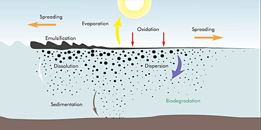
one for the spill size. Simulations performed for a real oil A schematic illustration of these effects can be seen in Fig. 1
spill case show that a minimum of approximately 80 % of (MEDESS-4MS, 2013; ITOPF, 2013). Also, as the spill ages,
the oil is captured by CranSLIK. Finally, Monte Carlo simu- different effects become more important – a speculative mass
lation is implemented to allow for consideration of the most balance can be seen in Fig. 2 (Mackay and McAuliffe, 1989).
likely destination for the oil spill, when the distributions for There are numerous equations created to model these effects,
the oceanographic conditions are known. based on both analytical and empirical approaches. However,
the complexity of the underlying physics is not yet fully un-
derstood. Reed et al. (1999) provide a very good summary of
early models. Since then significant progress has been made
1 Introduction in acquiring a deeper understanding of the involved complex
phenomena – for example biodegradation is studied by Mc-
Whilst the frequency of spills occurring has dropped signif- Genity et al. (2012).
icantly in the last few decades (Etkin, 2001), it does not di- Difficulty also arises as the result of uncertainty since ex-
minish the inevitability of an oil spill occurring. Oil spills act quantities are not necessarily known beforehand due to
can cause large-scale destruction of the environment, they the stochastic nature of certain variables, for example the sea
have significant economical effects, and can result in human surface velocity. The computational cost involved in running
life loss. They are inevitably the cause of environmental, eco- multiple cases, or Monte Carlo simulation, to consider the
nomic and human disaster. The Deepwater Horizon spill, for
Published by Copernicus Publications on behalf of the European Geosciences Union.1508 B. J. Snow et al.: Stochastic prediction of oil spill transport and fate Figure 1. Weathering process, from ITOPF (2013). possible conditions is often far too great to be a viable ap- proach. This becomes a severe impediment in cases of real accidents where a quick, or even real-time, prediction be- comes necessary. 1.1 MEDSLIK II Many models have been developed and used to predict the transport and transformation of an oil spill. These are either commercial, such as Li et al. (2013), or open-source, such as De Dominicis et al. (2013a). Regardless of the software tools employed, these models are not without their limita- tions. Often the computational cost involved in running a full simulation is too high. Alternatively, in order to be able to have a prediction in near real time, the model has to be sim- plified extensively, in terms of its physics, and therefore the simulation results are not of high accuracy. One such code is MEDSLIK II. This solves the advection– diffusion processes using a Lagrangian particle formalism, Figure 2. Speculative mass balance, from Mackay and McAuliffe meaning that the oil slick is broken into a number of con- (1989). stituent particles, while the transformation processes act on the entire oil slick surface. It has been shown to provide ac- curate results in a number of real scenarios (De Dominicis of the prediction over a 36 h period. The accuracy was found et al., 2013a; Coppini et al., 2011). Results are produced rea- to be in good agreement with the observed results (De Do- sonably quickly which is desirable since many simulations minicis et al., 2013a). This model has also been validated for are necessary to apply the regression model. the Lebanon crisis where the predicted oil slick at sea and There are four main inputs required: oil spill data, wind coastal deposits were in agreement with observations (Cop- field, sea surface temperature, and structure of sea currents. pini et al., 2011). The frequency of the oceanographic data is an important fac- Additional details regarding the development and valida- tor since these can change dramatically in a relatively short tion of MEDSLIK II can be seen in De Dominicis et al. period of time. MEDSLIK II applies a linear interpolation (2013a, b). in time between two subsequent current and wind fields to calculate the current and wind at the model time step. 1.2 Aims The test case included with the program is for an oil spill in Algeria. This consisted of 680 tonnes of crude oil being This paper investigates the use of stochastic methods to map spilled and validation was carried out to check the accuracy the response from different input variables to create a robust Geosci. Model Dev., 7, 1507–1516, 2014 www.geosci-model-dev.net/7/1507/2014/
B. J. Snow et al.: Stochastic prediction of oil spill transport and fate                                                            1509

and efficient software tool capable of effective prediction.         Pinardi et al. (2003) and Pinardi and Coppini (2010). The
This provides an estimation of the destination and spread            MFS system is composed of an Ocean General Circulation
of an oil spill subject to uncertain oceanographic conditions.       Model (OGCM) at 6.5 km horizontal resolution and 72 ver-
Also the minimal computational time required for the devel-          tical levels (Tonani et al., 2008; Oddo et al., 2009). Every
oped model allows for Monte Carlo simulation using non-              day MFS produces forecasts of temperature, salinity, inten-
deterministic values for current and wind velocities. This can       sity and direction of currents for the next 10 days. Once
then be used to calculate a region such that there is a high         a week, an assimilation scheme, as described in Dobricic
probability that said region will contain the oil spill. This aids   and Pinardi (2008), corrects the model’s initial guess with
significantly in reducing the resultant financial and environ-       all the available in situ and satellite observations, produc-
mental cost of oil spills, predicting their likely development.      ing analyses that are initial conditions for 10-day ocean cur-
   Wind and current velocities are both continuous variables,        rent forecasts. The modelled currents and wind fields can be
and as such, it is impossible to investigate all possible val-       affected by uncertainties that arise from model initial con-
ues. Therefore, it is necessary to sample these variables. This      ditions, boundaries, forcing fields, parameterisations, etc. In
involves creating a discrete set of values which is represen-        this paper the hourly mean analyses have been used to elim-
tative of the continuous variable. The sampled values then           inate the additional uncertainty connected with forecasts for
create the set of necessary simulations called a design hyper-       both atmospheric and oceanographic input data.
cube (Myers et al., 2009).                                              Whilst many of these parameters may be measurable at
   The key steps in developing our methodology can be out-           the initial time, prediction of the oil spill destination requires
lined as follows:                                                    reasonable estimation of the conditions over the simulation
                                                                     period. There are numerous methods for circumventing this
    1. identify the key parameters and their relative distribu-      problem; usually the stochastic parameters are extrapolated
       tions necessary for short-term oil spill prediction;          from previous values – however, this can frequently cause
    2. sample the considered parameters to create a design hy-       gross errors. This hinders the accuracy of real time predic-
       percube;                                                      tion.
                                                                        In this problem, it is necessary to apply sampling to ensure
    3. generate simulation data using the design hypercube;          that the considered points are representative of the domain.
                                                                     This problem cannot be approached deterministically due to
    4. fit regression models to map the inputs to the response;
                                                                     the continuous nature of the parameters making the consider-
    5. use the aforementioned regression model to create a pre-      ation of every possible quantity unfeasible. There are numer-
       diction code;                                                 ous methods of sampling available. Monte Carlo simulation
                                                                     is the simplest. However, the associated high computational
    6. test the developed code against a real scenario and anal-     cost is a constraint in the context of the model development.
       yse the results.                                              Another alternative could be importance sampling, which
                                                                     adopts a Monte Carlo style simulation, but biases the out-
In order to generate simulation data, we have used the MED-
                                                                     put to favour areas of greater interest, for example the tails of
SLIK II model. This choice was based on a number of rea-
                                                                     the distribution. This, however, is also inappropriate since the
sons, but predominantly due to its robustness and because it
                                                                     entire distribution is of interest, and it is still relatively expen-
has been validated on multiple real spills as discussed in De
                                                                     sive. Instead, a Latin hypercube (LHC) method will be used,
Dominicis et al. (2013a, b).
                                                                     where the distribution is separated into blocks of equal prob-
                                                                     ability and then a random value is chosen from each block.
2    Uncertainties and stochastic modelling                          This has the advantage of requiring a smaller amount of nec-
                                                                     essary simulations to create a good design and hence is rela-
Another complexity in modelling arises from the uncertainty          tively inexpensive. The main disadvantage is that it does not
involved in prediction of oceanographic conditions and spill         necessarily guarantee a well-stratified design (Myers et al.,
parameters. Many parameters, which are known to have an              2009).
important role in the destination of an oil spill, are stochastic       A simple third-order polynomial regression model is used
in nature and therefore difficult to accurately predict.             to map the responses. It was found that lower-order models
   Wind forcing, i.e. the wind velocity components at 10 m           are too sensitive to the fluctuating component present in the
above the sea surface, is provided by meteorological mod-            simulation data. This is the same reason which prevents the
els, while currents and temperature are provided by oceano-          use of radius basis functions in place of a polynomial.
graphic models. The atmospheric forcing is provided by                  It is also possible that the input variables will possess
the European Centre for Medium-Range Weather Forecasts               cross-correlation. Therefore mixed variable terms, i.e. x1 x2 ,
(ECMWF), with 0.25◦ space, and 6-hour temporal resolu-               have to be included in the model.
tion. The current velocities used in this work come from
the Mediterranean Forecasting System (MFS) described in

www.geosci-model-dev.net/7/1507/2014/                                                     Geosci. Model Dev., 7, 1507–1516, 2014
1510 B. J. Snow et al.: Stochastic prediction of oil spill transport and fate
3 Methodology Table 1. Sampled values for centre of mass prediction.
As previously stated, the underlying physics of an oil spill is Wind magnitude Current magnitude Angle
very complex. Existing solvers require resolving many of the (in m s−1 ) (in m s−1 ) (in radians)
underlying phenomena. To perform direct simulations of all 0 0 0
possible conditions would be far too computationally expen- 2.0887 0.0505 π/4
sive. For example, MEDSLIK II requires several minutes per 5.7691 0.1497 π/2
run; 1000 runs using different input parameters would there- 6.1600 0.2488 3π/4
fore require many hours. Our approach avoids this problem 7.7913 0.3480 π
by creating a polynomial which maps inputs to a response 10.1252 0.4472 –
15.2786 0.5464 –
resulting in 1000 runs being possible in approximately 1 sec-
ond. This allows for consideration of likely destinations of
the oil spill using non-deterministic inputs. Note that the phe-
nomena which can be accounted for in CranSLIK are lim- wished to consider a value outside of the sampled range, ad-
ited to the phenomena modelled by MedSLIK II. The paper ditional simulations would have to be performed.
uses a non-intrusive method, whereby the regression model
is developed using the results from the solver, and does not 3.2 Sampling the variables
require being programmed into the solver itself. There are
To develop the model, it is necessary to sample the chosen
numerous benefits of this approach. Primarily it is performed
variables. In statistics and quantitative research methodol-
to simplify the problem. However, it also means that the de-
ogy, a data sample is a set of data collected and/or selected
veloped methodology can easily be applied to data from any
from a statistical population by a defined procedure. This has
source.
been done using the LHC technique, which involves splitting
the distribution into blocks of equal probability, then a ran-
3.1 Choice of variables dom value is chosen from each block. A brief experiment
was conducted and it was determined that a minimum of six
Three variables have been chosen: wind velocity, current ve- samples are required to capture a reasonably complex shape,
locity and spill size. the Weibull distribution. Note that it is not possible to predict
It is necessary to express each variable as a distribution. the shape of the resultant graph beforehand. However, it is
Spill size will simply be assumed uniform and various sizes expected to be more simple than the test shape. A zero point
tested. However, velocities need to be separated into two has also been considered for investigation of simulation noise
components: speed and angle. generated by MEDSLIK II. The variables have also been de-
The angle can then be simplified by treating the current an- coupled by consideration of a point mass oil spill subject to
gle as an axis and only looking at the wind angle with respect oceanographic conditions. The result was that the destination
to this axis. Also, symmetry can be applied, meaning that it can be determined by the current and wind velocities. It was
is only necessary to consider angles between 0 and π, since also found that the size of the spill depends on the initial spill
other angles are a reflection in the current axis. A uniform size as well as the spill age, that is time since initial spill.
distribution can then be assumed for this variable. The sampled values for wind and current velocities, and
The distribution for wind speed is widely accepted to the angles, can be seen in Table 1. Note that to simplify the
be reasonably well represented by a Weibull distribution required number of simulations, the developed model will
with shape and scale parameters 2.26 and 9.02 respectively displace the spill depending on the angle between the cur-
(de Prada Gil et al., 2012). Morgan et al. (2011) suggest that rent and wind velocities, with the current velocity treated as
a log-normal distribution is better for extreme wind speeds. an axis, and then translated to meaningful coordinates. Data
We are not looking at extreme speeds though, so the Weibull have been generated from the stated input values for a simu-
distribution is sufficient. It is somewhat more complicated to lation time of 36 h.
find a distribution for the current speed as this varies over the
globe. Since the pattern is almost entirely that of wind-driven 3.3 Response mapping
circulation, it is likely the same underlying distribution with
In order to map the responses, a third-order polynomial
varying coefficients based on location. Here, the current ve-
approximation was calculated using the method of least
locity for the test case has been analysed and a Weibull distri-
squares. It has been found that the zero-point fluctuations
bution superimposed, leading to the coefficients 1.9967 and
from the random walk procedure appear to skew the results
0.2132 for shape and scale respectively. The maximum ve-
disproportionally with lower-order models.
locity is limited by the highest sampled value. Performing
the prediction for a value outside the sampled range is not
recommended due to extrapolation errors. Therefore, if one
Geosci. Model Dev., 7, 1507–1516, 2014 www.geosci-model-dev.net/7/1507/2014/B. J. Snow et al.: Stochastic prediction of oil spill transport and fate 1511
3.4 Developed methodology
Once the polynomials have been created, it is necessary
to outline the developed methodology for prediction of an
oil spill, using the calculated coefficients. The flow chart
of the developed model can be seen in Fig. 3. The actual
code has been written in the commercial software package
MATLAB® (2011) and the statistics toolbox is used for the
Monte Carlo simulation to generate the random numbers.
An overview of the methodology is as follows:
– Interpretation of oceanographic data. The key parame-
ters in the prediction are the wind and current velocities.
MEDSLIK II produces column-structured data for these
from the raw NetCDF files. The prediction code is capa-
ble of reading these and converting them to block struc-
ture and converting from latitude and longitude to me-
tres. A modified version of this code has also been writ-
ten for the purposes of Monte Carlo simulation, where
the user inputs a desired wind and current velocity di-
rectly.
– Centre of mass. To investigate the behaviour of the
centre of mass, the wind, current and angle variables
have been considered. A polynomial has been devel-
oped which links these variables to predict displacement
in the x and y planes. The oceanic data are interpolated
to find the parameters at the spill location and these are
fed into the regression model to predict a new centre.
Since the current direction is treated as an axis, the dis-
placement with respect to this is first calculated, and
then translated into more meaningful coordinates.
Figure 3. Flowchart of the developed model.
– Reconstruction of surface. Now the centre of mass has
been predicted, the surface reconstruction of the oil spill
For the spill size, a slightly different approach was taken, can be considered. Since this is not linked to the destina-
where the developed equation comes from r = g(θ), i.e. a ra- tion of the centre of mass, the rings are created around
dial function is developed, as opposed to a Cartesian. This the origin and then displaced by the calculated displace-
assists in ensuring a periodic, or near-periodic model. Note ment of the centre of mass. If desired, a contour can then
that both a polynomial and sinusoidal functions were inves- be fitted according to these concentration rings. These
tigated and the polynomial appears to produce less skewed are fourth-order polynomials and require the initial spill
results in the central region and hence the polynomial func- size (tonnes) and the spill age (hours).
tion was chosen. But as outer rings are of greater interest,
either choice could be acceptable. – Set values for next iteration. For the next time step, it is
Seven values have been sampled for the wind and current necessary to set the new centre of mass for the oil spill.
magnitudes, however only five angles have been considered. At this stage, the centre of mass can be corrected based
This is because the angle refers to the angle between the wind on observation to produce more accurate results.
and current velocities, and since the current velocity is used
as an axis, symmetry can be applied to reduce the number of 4 Case study
necessary values in this parameter. Therefore five values over
a semi-circle are chosen, which corresponds to eight values In order to validate CranSLIK, it is necessary to investigate
over a circle. its performance when applied to oceanographic conditions.
The accuracy of CranSLIK is evaluated by the volume of oil
captured, where this is calculated as the volume of oil ex-
plained by the model, divided by the total oil volume. Note
that the model has been verified against the sampled points
www.geosci-model-dev.net/7/1507/2014/ Geosci. Model Dev., 7, 1507–1516, 20141512 B. J. Snow et al.: Stochastic prediction of oil spill transport and fate
Figure 4. Proportion of oil captured using different update frequen- Figure 5. Centre of mass prediction using different update frequen-
cies. cies.
and that over 99.5 % of the oil was captured for each case
after 1 h of simulation. It was also found that the prediction
becomes less accurate for extended periods. The wind and
current velocities were both found to produce near-linear dis-
placement with respect to time, when considered individu-
ally. The developed model works by hourly prediction which
causes cumulative errors in extended simulation. Hindcast
modelling, updating the centre of mass every hour, is there-
fore recommended to minimise error. The spill size predic-
tion remains very accurate, above 99 %, over a 36 h period
suggesting that hindcast modelling is not required to be ap-
plied to this part of the code.
4.1 Algeria test case
Figure 6. Proportion of oil captured by the spill size prediction only,
The case considered uses the oceanographic data for the Al- for the Algeria scenario.
geria spill on 6 August 2008 and a point mass oil spill is
released from latitude 38.240◦ and longitude 5.981◦ . Current
velocities were updated every hour and wind velocities every Figure 5 shows the displacement error of the centre of
6 h. It is found that the proportion of oil captured becomes mass, when this value is updated at different intervals. It is
poor when a full 36 h prediction is performed – the accuracy clear that the error is far smaller when the simulation is only
rapidly drops after the 4 h mark as shown in Fig. 4. However, predicting for an hour and then updating.
under the application of hindcast modelling, where the cen- With regard to the spill size only, the accuracy appears to
tre of mass is updated every hour based on model data, the be very good, as seen in Fig. 6. Compared to the accuracy of
minimum accuracy is greatly improved. This is likely due to the centre of mass prediction, this appears to be far more ac-
cumulative errors during prediction. These errors could be curate, suggesting that the weakest component of this model
present in the developed model. However, since the model is the centre of mass prediction; however, the overall accu-
has been verified, it may be an error due to the oceanographic racy appears to be reasonably good – a minimum of 80 %
data. The model assumes that the oceanographic conditions when hourly prediction is used as seen in Fig. 4. This also
at the start of the simulation period are representative of the justifies the decoupling of variables.
conditions over the period. This however is not necessarily The supplementary animation shows the predicted oil spill
true and therefore the prediction is less accurate when these (black rings) and the MEDSLIK II result (background con-
conditions change greatly over the simulation period. It is tour) for a 36 h simulation period for this test case. The centre
possible in this case to apply an interpolation since the quan- of mass for the prediction is updated every hour. The lowest
tities for the next time step are known. However, this would proportion of oil captured is approximately 80 % with the av-
not be possible in a real scenario. erage being about 91 %.
Geosci. Model Dev., 7, 1507–1516, 2014 www.geosci-model-dev.net/7/1507/2014/B. J. Snow et al.: Stochastic prediction of oil spill transport and fate 1513
Table 2. Sensitivity of variables for the first hour of the Algeria 4.4 Discussion
scenario. Upper and lower ranges for 90 % accuracy are given.
Whilst CranSLIK appears to perform well for the tested sce-
Variable Lower limit Upper limit Observed narios, it is necessary to identify the assumptions made while
Wind magnitude −2.0423 9.3860 4.3454
modelling. Firstly, the displacement of the centre of mass is
Current magnitude 0.0065 0.1130 0.0653 correlated to the wind and current velocities only, while the
Wind angle −2.5844 −0.2280 −1.5202 spill area is determined by the quantity of oil spilled and the
Current angle −1.7279 −0.6605 −1.4048 age. Although these variables are considered dominant, in a
Spill size 163.2 NA 680 fully robust model further simulations considering different
variables should be performed. This would lead to an even
more accurate prediction. However, it would require more
complicated approximations to account for these variables
4.2 Sensitivity analysis and their correlations. Additional variables could be included
to account for more complicated flow physics such as non-
It is also of interest to consider the sensitivity of CranSLIK radial oil spill expansion. Secondly, rather than the MEDS-
with respect to the different input parameters. This is sum- LIK II which was employed, other oil spill prediction codes
marised in Table 2. and softwares may be used and compared to identify their
The most sensitive variables appear to be the current mag- performance in aspects of accuracy and computational ef-
nitude and angle. This is expected since the displacement due fort and at the same time highlight efficiency of the proposed
to current velocity is far greater than that due to the wind ve- non-intrusive methodology. Finally, only one particular type
locity, and since the majority of the oil is contained close to of oil spill has been considered: point-mass. Since the devel-
the centre, the dispersed elements do not skew the results sig- oped model moves a centre of mass, and then reconstructs the
nificantly and hence there is some leeway with the spill size. surface, it is possible to mark several centres of masses and
This was expected since the current is more displacing than predict their destinations. The problem then becomes surface
the wind, and it was concluded the wind is less important reconstruction which would require additional simulations.
when the sensitivity of variables was investigated in MEDS- As with any stochastic problem, additional simulations could
LIK II (De Dominicis et al., 2013a). lead to a better regression fit and hence better prediction.
4.3 Monte Carlo simulation
5 Conclusions
CranSLIK assumes that the wind and current data at the start
of the hour are representative of the full hour. This, however, This paper describes the development of CranSLIK, a model
is not necessarily true since oceanographic conditions may for the prediction of the destination and spread of an oil spill
change. Therefore, more accurate prediction may be possible via a stochastic approach. The key parameters were identi-
if an interpolation is applied to the data and expected fields fied as wind velocity, current velocity, spill size and time,
are created. However, this is not relevant for prediction of and a design square was created for the required samples.
real-time oil spills. In such scenarios it may be of interest to The simulations were then performed using MEDSLIK II
generate an expected region for the oil spill. and regression modelling was applied to create two equa-
Due to the incredibly low computational cost required by tions: one to predict the centre of mass, and one to predict
CranSLIK, a Monte Carlo simulation can be performed in the spill size. The developed code has been presented and
a very low time frame, approximately 1000 simulations per discussed. It was then validated against a real test case. Fi-
second on an AMD Phenom II X4 3.6 GHz processor. This nally, the efficiency of the model is exploited using Monte
can be used to generate an expected region for the oil spill Carlo simulation for the purposes of generating maximum
and aid in clean-up and recovery operations. likelihood regions. This has limited use when applied to the
For the Algeria test case, the Monte Carlo simulation was Algeria test case due to insufficient current and wind velocity
performed using input distributions developed from the avail- data to more accurately fit a distribution. Note that CranSLIK
able data. However, due to the 60 h period of data, there ex- is limited to the same physical phenomena which are mod-
ists a bimodal peak in the simulation results representative elled by MEDSLIK II.
of the alternating current forcing as shown in Fig. 7. This be- The developed model appears to perform well when ap-
comes clearer when the simulation is performed using 10 000 plied to the Algeria test case considered, with a minimum
and 100 000 samples, as shown in Figs. 8 and 9 respectively. of 80 % of the oil captured when using hourly prediction.
This result is not too helpful because of the bimodal peak. The major strength of the developed model is the efficiency
However, it does demonstrate the versatility and robustness and the minimal time required to perform Monte Carlo sim-
of CranSLIK. If the distribution for a location is known, more ulation and generate maximum likelihood regions. However,
meaningful results can be produced. for this to provide useful results, it is necessary to have
www.geosci-model-dev.net/7/1507/2014/ Geosci. Model Dev., 7, 1507–1516, 20141514 B. J. Snow et al.: Stochastic prediction of oil spill transport and fate
2.61746
2500
2.35571
2000
2.09397
1500 1.83222
y Displacement, m
1.57048
1000
1.30873
500
1.04698
0 0.785238
0.523492
−500
0.261746
−1000
−2500 −2000 −1500 −1000 −500 0 500 1000 1500 2000
x Displacement, m
Figure 7. Monte Carlo simulation of the Algeria test case contoured by cell frequency, 1000 iterations, 1 h simulation.
1400 4.58127
1200 4.12314
1000 3.66502
800 3.20689
y Displacement, m
600 2.74876
400 2.29064
200 1.83251
0 1.37438
−200 0.916254
0.458127
−400
−2000 −1500 −1000 −500 0 500 1000 1500 2000
x Displacement, m
Figure 8. Monte Carlo simulation of the Algeria test case contoured by cell frequency, 10 000 iterations, 1 h simulation.
a distribution or a reasonable estimate of expected oceano- Whilst the key variables were considered, it has been identi-
graphic conditions. This paper serves as a demonstration of fied that consideration of additional variables could result in
an alternative method for fast prediction of the advection– improved accuracy.
diffusion–transformation of an oil spill. The assumptions
have been discussed and areas for further work highlighted.
Geosci. Model Dev., 7, 1507–1516, 2014 www.geosci-model-dev.net/7/1507/2014/B. J. Snow et al.: Stochastic prediction of oil spill transport and fate 1515
17.6925
1200
15.9233
1000
14.154
800
12.3848
600
y Displacement, m
10.6155
400
8.84627
200
7.07702
0
5.30776
−200
3.53851
−400
1.76925
−600
−1000 −500 0 500 1000
x Displacement, m
Figure 9. Monte Carlo simulation of the Algeria test case contoured by cell frequency, 100 000 iterations, 1 h simulation.
Code availability References
The oil spill model code CranSLIK v1.0 is available as an
open source code that can be downloaded together with test Coppini, G., De Dominicis, M., Zodiatis, G., Lardner, R., Pinardi,
case data and output example from the website http://public. N., Santoleri, R., Colella, S., Bignami, F., Hayes, D. R., Soloviev,
cranfield.ac.uk/e102081/CranSLIK. CranSLIK is available D., Georgiou, G., and Kallos, G.: Hindcast of oil-spill pollution
under the GNU General Public License (GNU-GPL Version during the Lebanon crisis in the Eastern Mediterranean, July–
3, 29 June 2007). The code is written in the commercial soft- August 2006, Marine Pollut. Bull., 62, 140–153, 2011.
ware package MATLAB® (2011). The model code can run De Dominicis, M., Pinardi, N., Zodiatis, G., and Archetti, R.:
on any computer and operating system that supports Matlab. MEDSLIK-II, a Lagrangian marine surface oil spill model for
short-term forecasting – Part 2: Numerical simulations and vali-
dations, Geosci. Model Dev., 6, 1871–1888, doi:10.5194/gmd-6-
1871-2013, 2013a.
The Supplement related to this article is available online
De Dominicis, M., Pinardi, N., Zodiatis, G., and Lardner, R.:
at doi:10.5194/gmd-7-1507-2014-supplement.
MEDSLIK-II, a Lagrangian marine surface oil spill model for
short-term forecasting – Part 1: Theory, Geosci. Model Dev., 6,
1851–1869, doi:10.5194/gmd-6-1851-2013, 2013b.
de Prada Gil, M., Gomis-Bellmunt, O., Sumper, A., and Bergas-
Jane, J.: Power Generation efficiency analysis of offshore wind
Acknowledgements. We gratefully acknowledge the two anony-
farms connected to SLPC (simgle large power converter) oper-
mous reviewers and the topical editor, Robert Marsh, for providing
ated with variable frequencies considering wake effects, Energy,
constructive comments that improved this paper. The service
37, 455–468, 2012.
charges for this open access publication have been covered by
Dobricic, S. and Pinardi, N.: An oceanographic three-dimensional
Cranfield University.
variational data assimilation scheme, Ocean Model., 22, 89–105,
2008.
Edited by: R. Marsh
Etkin, D. S.: Analysis of oil spill trends in the United States and
worldwide, in: International Oil Spill Conference Proceedings,
1291–1300, 2001.
Graham, B., Reilly, W. K., Beinecke, F., Boesch, D. F., Garcia,
T. D., Murray, C. A., and Ulmer, F.: Deep Water: The Gulf Oil
Disaster and the Future of Offshore Drilling: Report to the Pres-
ident, United States Government Printing Office, 2011.
www.geosci-model-dev.net/7/1507/2014/ Geosci. Model Dev., 7, 1507–1516, 20141516 B. J. Snow et al.: Stochastic prediction of oil spill transport and fate ITOPF: Weathering Process, Online, available at: http://www. Oddo, P., Adani, M., Pinardi, N., Fratianni, C., Tonani, M., and Pet- itopf.com/marine-spills/fate/weathering-process/, last access: tenuzzo, D.: A nested Atlantic-Mediterranean Sea general circu- 13 May 2013. lation model for operational forecasting, Ocean Sci., 5, 461–473, Li, W., Pang, Y., Lin, J., and Liang, X.: Computational Modelling doi:10.5194/os-5-461-2009, 2009. of Submarine Oil Spill with Current and Wave by FLUENT, Pinardi, N. and Coppini, G.: Preface “Operational oceanography in Research Journal of Applied Sciences, Eng. Technol., 5, 5077– the Mediterranean Sea: the second stage of development”, Ocean 5082, 2013. Sci., 6, 263–267, doi:10.5194/os-6-263-2010, 2010. Mackay, D. and McAuliffe, C. D.: Fate of hydrocarbons discharged Pinardi, N., Allen, I., Demirov, E., De Mey, P., Korres, G., Las- at sea, Oil Chemical Pollut., 5, 1–20, 1989. caratos, A., Le Traon, P.-Y., Maillard, C., Manzella, G., and MATLAB® : version 7.12.0.635 (R2011a), The MathWorks Inc., Tziavos, C.: The Mediterranean ocean forecasting system: first Natick, Massachusetts, 2011. phase of implementation (1998–2001), Ann. Geophys., 21, 3–20, McGenity, T., Folwell, B., McKew, B., and Gbemisola, S.: Marine doi:10.5194/angeo-21-3-2003, 2003. crude-oil biodegradation: a central role for interspecies interac- Reed, M., Øistein Johansen, Brandvik, P. J., Daling, P., Lewis, A., tions, Aquatic Biosystems, 8, 1–19, 2012. Fiocco, R., Mackay, D., and Prentki, R.: Oil Spill Modeling to- MEDESS-4MS: Weathering Process, Online, available at: http:// wards the Close of the 20th Century: Overview of the State of www.medess4ms.eu/marine-pollution, last access: 13 May 2013. the Art, Spill Sci. Technol. Bull., 5, 3–16, 1999. Morgan, E. C., Lackner, M., Vogel, R. M., and Baise, L. G.: Prob- Tonani, M., Pinardi, N., Dobricic, S., Pujol, I., and Fratianni, C.: ability distributions for offshore wind speeds, Energy Conserv. A high-resolution free-surface model of the Mediterranean Sea, Manage., 52, 15–26, 2011. Ocean Sci., 4, 1–14, doi:10.5194/os-4-1-2008, 2008. Myers, R. H., Montgomery, D. C., and Anderson-Cook, C. M.: Re- sponse Surface Methodology, John Wiley and Sons, 3rd Edn., 2009. Geosci. Model Dev., 7, 1507–1516, 2014 www.geosci-model-dev.net/7/1507/2014/
You can also read