A Logistic Regression Based Auto Insurance Rate-Making Model Designed for the Insurance Rate Reform - MDPI
←
→
Page content transcription
If your browser does not render page correctly, please read the page content below
International Journal of
           Financial Studies

Article
A Logistic Regression Based Auto Insurance
Rate-Making Model Designed for the Insurance
Rate Reform
Zhengmin Duan 1, *, Yonglian Chang 1 , Qi Wang 1 , Tianyao Chen 2 and Qing Zhao 3
 1    College of Mathematics and Statistics, Chongqing University, Chongqing 401331, China;
      a410727199@126.com (Y.C.); eternalgrace7@163.com (Q.W.)
 2    College of Mathematics and Statistics, Xi’an Jiaotong University, Xi’an 710000, China; busydoris@sina.com
 3    Lingnan College of Sun Yat-sen University, Guangzhou 510000, China; graceki7@163.com
 *    Correspondence: dzm@cqu.edu.cn; Tel.: + 86-136-2830-1158

 Received: 13 November 2017; Accepted: 1 February 2018; Published: 7 February 2018

 Abstract: Using a generalized linear model to determine the claim frequency of auto insurance is a
 key ingredient in non-life insurance research. Among auto insurance rate-making models, there are
 very few considering auto types. Therefore, in this paper we are proposing a model that takes auto
 types into account by making an innovative use of the auto burden index. Based on this model and
 data from a Chinese insurance company, we built a clustering model that classifies auto insurance
 rates into three risk levels. The claim frequency and the claim costs are fitted to select a better loss
 distribution. Then the Logistic Regression model is employed to fit the claim frequency, with the
 auto burden index considered. Three key findings can be concluded from our study. First, more
 than 80% of the autos with an auto burden index of 20 or higher belong to the highest risk level.
 Secondly, the claim frequency is better fitted using the Poisson distribution, however the claim cost is
 better fitted using the Gamma distribution. Lastly, based on the AIC criterion, the claim frequency is
 more adequately represented by models that consider the auto burden index than those do not. It is
 believed that insurance policy recommendations that are based on Generalized linear models (GLM)
 can benefit from our findings.

 Keywords: auto insurance; claim frequency; logistic regression model

1. Introduction
      As of 2016, the amount of total property insurance premiums continues to increase, which makes
total property insurance the biggest part in the property insurance industry.
      At present, the international approaches of rate making are mainly chauvinism and humanitarianism.
Traditional Chinese insurance companies are mainly from chauvinism, which is the value of the car
itself. However, with the development of the insurance industry, the existing provisions begin to
consider human factors, including driving record, driver’s age, family members, regional factors and
so on. This is more conducive to the mobilization of the driver’s initiative, making the burden of
insurance premium more reasonable.
      China market reform of auto insurance rate has been a few twists and turns. On 1 June 2015,
as one of the six pilot areas for deepening the reform of the auto insurance rate management system
in China, Chongqing officially started the commercial terms for the reform of the auto insurance rate
management system.
      The main content of the rate reform is that after adjustment, a total of four rate adjustment
coefficients under the new tariff system are determined, including bonus-malus coefficient (NCD),
independent channels coefficient, autonomous underwriting coefficient, the traffic law coefficient and

Int. J. Financial Stud. 2018, 6, 18; doi:10.3390/ijfs6010018                         www.mdpi.com/journal/ijfs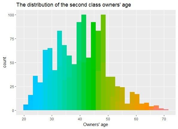
Int. J. Financial Stud. 2018, 6, 18                                                                  2 of 16

the client discount coefficient. Especially the independent channels coefficient and autonomous
underwriting coefficient are the embodiment of pricing power for the insurance companies to
choose. After the reform, the risk of financial insurance companies expanded, putting forward
higher requirements for the management strategy of insurance companies.
     Therefore, it is of great significance to discuss the reform of auto insurance rates. According
to the regulations of the new reform, auto burden index will be introduced to quantify the model
analysis. And the auto insurance rate-making is studied on the basis of practical data. Firstly, cluster
analysis was used to classify the risk categories into three kinds of risk categories according to the
age of owners, vehicle age and vehicle burden index. After the reform, the insurance company may
set different business car insurance rates, according to their own risk recognition, risk cost and risk
pricing power, motor vehicles and drivers of different risk levels. The improvement of the pricing
power of insurance companies and the increase of consumers’ satisfaction have confirmed the initial
success of the commercial car insurance reform.
     The paper is organized as follows. In Section 2, the data and the auto burden index are introduced.
The results of the cluster analysis are discussed in Section 3. In Section 4, the selection procedure of the
loss distribution is presented and the preferred distributions for both claim frequency and claim cost
are given. In Section 5, the claim frequency is fitted by logistic regression model considering the auto
burden index. A conclusion for our proposed method is drawn in Section 6.

2. International Research Background
      Risk classification plays a part to eliminate cross-subsidy between people with low and high
risks, which contributes to promote the market efficiency, as well as the increase of social risk
cost and the loss of fairness. The impact on equity and efficiency in the insurance market has
always been the focus of debate. The first study of the risk classification is Hoy (1982), the R-S
equilibrium, Wilson equilibrium and Miyazaki’s assumption are expected as the underwriter contracts
in the cross-subsidy equilibrium model, the results showed that the causal relationship between risk
classification and economic efficiency is not clear, which depends on the classification and form of
equilibrium. Crocker and Snow (1986) made more detailed studies, they did not categorize the groups
in the utility of boundary classification, otherwise, they came to the following conclusions. First, any
market equilibrium with no cost classification is better than that of without classification. Second,
it is not easy to measure fairness and efficiency of resource costs according to classification and it
may be effective to ban some sort of cost classification. Lereah (1983) and Cheng (2007) compared the
effects of different risk classification subjects. They believed that there are two options for insurance
companies to classify the insured, one is that the insurance company is independent and the other
is the risk assessment institution. The two schemes differ in cost and accuracy. The risks in auto
insurance were classified by cluster analysis in this paper. Since the beginning of the 20th century, some
scholars have studied non-life actuarial models. The classification rate, general rate and individual
risk rate are the main non-life insurance pricing methods. Among them, classification rate is a kind of
non-life insurance pricing method based on risk classification, which has a certain universality and
is not lack of pertinence to specific groups. Finger (2001) of this method has carried on the detailed
narration, more scientifically expounds the classification rate set: the basic idea of the large number of
individuals with homogeneous risk is divided into the same category, through the statistical method
to determine the relative abundance of each group level and the corresponding parameters and then
get the group rate. In 1960, Bailey and Simon (1960) believed that the basis of classification rates was
to group individuals of the same risk characteristics, determine the relative number of risk levels of
each group and then calculate relative rates. Bailey (1963) presented a single analysis method to study
the impact factors of single rate on policy prices. On this basis, Holler et al. (1999) summed up to
determine the level of the relative abundance of three basic methods, namely the minimum deviation
method, maximum likelihood method and loss relative ratio method, at the same time points out the
defects of various methods.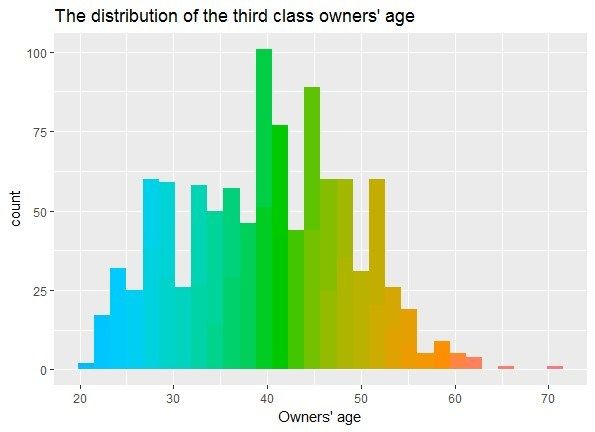
Int. J. Financial Stud. 2018, 6, 18                                                                           3 of 16

     Generalized linear model (GLM) is the earliest by Nelder and Wedderburn (1972) put forward
and give a specific definition, in the aftermath, Anderson et al. (2004) of the generalized linear
model of exponential distribution density function and the form of moment generating function are
discussed and the specific distribution types of exponential distribution family, such as the gamma
distribution, poisson distribution is introduced in detail. McCullagh et al. first applied GLM to the
actuarial field. Since then, GLM has been widely used in non-life insurance rates and has become a
standard method for auto insurance rates. However, with the development of actuarial theory and the
practice of premium rate making accuracy requirement for further improve, GLM also exposed some
defects in the application, therefore scholars on the many kinds of extension. Pregibon et al. (1984)
proposed a dual generalized linear model (DGLM) that established the model of the mean and
divergence parameters of the reaction variables and extended the traditional generalized linear model
further. Smyth introduces the maximum likelihood estimation of DGLM and considers the situation
of normal and inverse Gaussian distribution. Smyth applies DGLM to non-life insurance pricing
and forecasts the rate of vehicle loss but excludes regional factors in empirical research and the rate
structure is not reflected in regional differences. In terms of application of premium rate making model,
Aitkin et al. (1989) studied a lot of application examples of generalized linear models, including the
poisson distribution is used to simulate insurance claims data for multiple vector list in the distribution
of cell count Ohlsson and Johansson (2010) introduced the generalized linear model in the practical
application in automobile insurance, through empirical analysis, data selection for claim frequency
poisson distribution model, to choose a claim intensity gamma distribution model in fitting, gives a
detailed introduction and rigorous derivation.

3. Data
      After the reform of auto insurance rate system in China, 2015, the insurance companies determined
auto insurance rates for autos and drivers with different risk levels, considering the factors including
risk identification capabilities, risk costs, risk pricing capabilities. Based on the new regulations of the
reform, we used the data of an insurance company in Chongqing, China, with a total of 33,373 sets of
insurance policies, ensuring the authenticity and effectiveness in the analysis. While Adriana Bruscato
Bortoluzzo (2011) classified the auto types into luxury, medium and small with an index respectively.
In this article, we introduce the auto burden index into the model to precisely quantify the auto types,
transforming the auto types into specific values, which is described by the formula,

              Single commonly used accessories price × accessories loss rate ÷ auto sales price × 100

     The insurance policy mainly includes claims frequency last year, license plate numbers, auto age,
owners’ age and the settled claims. The auto burden index in this article was jointly issued by China
Insurance Industry Association and China Automobile Maintenance Industry Association, with a total
of 526 auto burden indexes of the commonly used auto types. After removing the insurance policies
with undefined auto burden index or missing data, the remained 2783 sets of insurance policies were
used as experimental data.

The Statistical Verification of the Auto Burden Index
     The higher the burden index, the higher the claim amount. The higher the index, the better
the overall performance of the auto is and the lower the accident rate is. Consequently, the claims
frequency is negatively correlated with the auto burden index. The latter part of the empirical test also
validates this view. The overall significance function of the model is

                                                                                  e β0 + β1 x1 +··· βr xr
                                      p = E ( y = 1| x1 , x2 , · · · , xr ) =
                                                                                1 + e β0 + β1 x1 +··· βr xr
    The function is an incremental function, the auto burden index and the claim frequency is
negatively correlated. The decrease of p value indicating an increase in the model significance.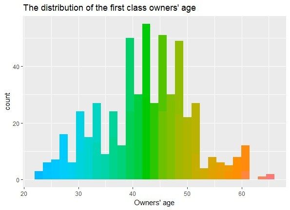
Int. J. Financial Stud. 2018, 6, 18                                                                    4 of 16

4. Classification of Risks—Cluster Analysis
       Risk classification refers to that the insurer can distinguish between high-risk and low-risk
policyholders based on the variables containing the risk information of policyholders. If high-risk and
 low-risk policyholders can be completely distinguished, it is called complete classification. Otherwise,
 if there are a small number of low-risk policyholders in the high-risk group after the risk classification,
 or a small number of high-risk policyholders in the low-risk group, it is called incomplete classification.
       In the auto insurance business, it is necessary to assess the risk of the policy amount and classify
 the risks of the insured, which are called the classification rates. The selected risk determinants are
 also called rate factors. Cluster analysis is an unsupervised learning process for finding similar sets of
 elements in a data set. The common feature of this method is that when the number and structure of
 the classes are unknown, the similarity between these data is measured by a certain distance criterion.
The information of the insured (age, gender, etc.), the information of the auto (auto type, age, etc.),
 the claim frequency and the settled claim are in close connection with each other, it’s important to find
 out their relations in the classification. In this article, the information of the insured is clustered and
 different characteristics of types are obtained and the decision support is provided to the insurance
 company through the analysis. xij represents a latent variable by the candidate in sample i and indicator
 j, each sample has p variables, we selected six variables for each sample, including the ‘total signed
premium,’ ‘owners age,’ ‘the claim frequency last year,’ ‘settled claim,’ ‘the auto burden index’ and
‘auto age.’ We use xj and ri to denote the variable j and the sample i respectively, dij is used to express
 the distance between sample i and the sample j. Comparing with the common distances, it’s easy to find
 out that the real data is better fitted with the European distances, which is described by formula as:
                                                    v
                                                    u p
                                              dij = t ∑ ( xik − x jk )2
                                                    u

                                                        k =1

     Regarding each sample as a separate class, the basic ideas of system cluster are as follows: first
specify the distances between samples and the distances between classes, secondly merge the nearest
two classes into a new class, then calculate the distance between the new classes and the other classes,
repeating the merger of the nearest two classes until all the samples are merged into one class. dij
represents the distance between the sample i and the sample j, G1 and G2 represent classes and DKL
represents the distance between the class K and the class L. The Ward method is used to system cluster
in this article. Based on the idea of variance analysis, if the classification is correct, the sum of squares
between the same classes should be small, the sum of squares between different classes should be
large. The number of samples in this paper is large, the two classes tend to have a relatively large
distance, so we choose the Ward. Suppose GK and GL are merged into a new class, the sum of squares
of GK , GL and GM are as follows:

                                       WK = ∑ ( x(i) − xK ) T ( x(i) − xK )
                                               i ∈ GK
                                       WL = ∑ ( x(i) − x L ) T ( x(i) − x L )
                                               i ∈ GL
                                      WM = ∑ ( x ( i ) − x M ) T ( x ( i ) − x M )
                                              i∈GM

    The above formulas reflect the dispersion degree of the samples in each class and the sum of
squares between GK and GL is:
                                    DKL2 = W M − W K − W L

     In this section, the data is clustered by R software and the 2783 sets of data are divided into three
classes, 1–536 for the first class and 537–1760 for the second class, the remaining as the third category.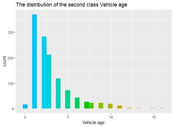
Int. J. Financial Stud. 2018, 6, 18 5 of 16
Int. J. Financial Stud. 2018, 6, x FOR PEER REVIEW 5 of 16
Int. J. Financial Stud. 2018, 6, x FOR PEER REVIEW 5 of 16
4.1.4.1.
The Distribution
The Distributionofofthe
theTotal
TotalSigned
SignedPremium
Premium and
and the
the Settled Amount
Amount
4.1.After
The Distribution
clustering,
After ofthe
clustering,thethe Total
total
total Signedpremium
signed
signed Premium is
premium and the Settled
classified
classified Amount
into
into thethree
the threeclasses,
classes,
asas shown
shown in Figure
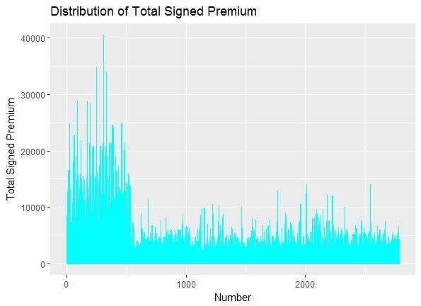
in Figure 1. 1.
After clustering, the total signed premium is classified into the three classes, as shown in Figure 1.
Figure1.1.Distribution
Figure Distribution of
of the
the total
totalsigned
signedpremium.
premium.
Figure 1. Distribution of the total signed premium.
Since the raw data is provided by the insurance company with better practical significance on
Since
the market,thewe rawcandatasee is provided
that the totalby the insurance
signed premium of company with
the firstwith betterispractical
classbetter
1–536 much highersignificance
than the on
Since the raw data is provided by the insurance company practical significance on
theother
market,
two we can see that thethe
classes. total
firstsigned premium of the first class 1–536 is much higher than athe
the market, we canTherefore,
see that the total class should
signed premium be regarded
of the firstasclass
a high-risk
1–536 isclass,
muchwhich
higherrequires
than the
other two classes. Therefore, the first class should be regarded as a high-risk class, which requires a
other two classes. Therefore, the first class should be regarded as a high-risk class, which requires aa
higher premium. The second class 537–1760 should be regarded as a low-risk class, which requires
higher
lowerpremium.
higher premium.The
premium. Thesecond
The total
second class
signed 537–1760
classpremium
537–1760of should be regarded
the third
should be regarded asaalow-risk
class 1761–2783
as low-risk
is smallerclass,
class,thanwhich requires
therequires
which first classa a
lower
but premium.
the volatilityThe
is total
greater signed
than premium
the second of the
class, sothird
that class
the 1761–2783
second class is
can
lower premium. The total signed premium of the third class 1761–2783 is smaller than the first class smaller
be than
regarded the
as first
uncertainclass
butbut
thethe
risk volatility
class, isisgreater
which
volatility than
requires
greater the
thesecond
thanbeing class,
discussed
second so that the
further.
class, so that the
Thesecond
settled
second classamount
class cancanbebe regarded
is the as
regarded as uncertain
cumulative
uncertain
risk class,
risk which
compensation
class, requires
amount
which ofbeing
a case
requires discussed
that has
being further.
been
discussed The
filed andsettled
further. Theamount
closed, which is
settled the cumulative
plays
amount is the compensation
an important role in the
cumulative
operating
amount income
case that of
hasthe insurance
been filed and company,
closed, including
which plays the
an cumulative
compensation amount of a case that has been filed and closed, which plays an important role inincome
of a important compensation
role in the amount
operating of
the
payment
of operating that
the insurance has been
company, closed and
including paid
the out of or
cumulative has been closed
compensation and
income of the insurance company, including the cumulative compensation amount of unpaid.
amount of The settled
payment amount
that has is
been
classified
closed
payment according
and paid out been
that has to the
of or closedclustering
has been andclosed result,
paid out as shown
andofunpaid. in Figure
The settled
or has been 2.
closed amount
and unpaid. is classified according
The settled amounttoisthe
classifiedresult,
clustering according
as shownto thein clustering
Figure 2.result, as shown in Figure 2.
Figure 2. Distribution of the settled amount.
Figure2.2. Distribution
Figure Distribution of
of the
the settled
settledamount.
amount.
According to Figure 2, the distribution of the settled amount is consistent with the distribution
of theAccording
total signed premium.
to Figure Therefore,
2, the it can
distribution be generally
of the considered
settled amount that thewith
is consistent first the
class should be
distribution
According
regarded as a to Figure class,
high-risk 2, thethe
distribution
second andofthe
thethird
settled amount
class still is consistent
need further with the
analysis. distribution
According to
of the total signed premium. Therefore, it can be generally considered that the first class should be
of regarded
the above
the total signed
as a high-risk class, the second and the third class still need further analysis. According to be
premium.
classification Therefore,
results, we will it can
further be generally
discuss the considered
classification that
of the first
variables. class should
regarded as a high-risk class,
the above classification thewe
results, second and the
will further third the
discuss class still need further
classification analysis. According to
of variables.
the above classification results, we will further discuss the classification of variables.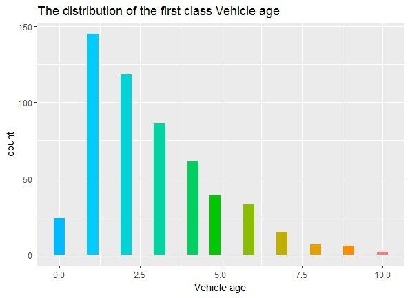
Int. J. Financial Stud. 2018, 6, 18                                                                                    6 of 16

4.2. Analysis of the Variable Classification
      Int. J. Financial Stud. 2018, 6, x FOR PEER REVIEW                                                         6 of 16
4.2.1. Burden Index
      4.2. Analysisto
      According     of the
                       theVariable Classification
                           classification   of the auto burden index, the results as shown in Table 1.
      4.2.1. Burden Index
                                  Table 1. Distribution of the auto burden index.
            According to the classification of the auto burden index, the results as shown in Table 1.
                                      0–10                    10–20                   20–30                 Above 30
     Burden Index
                          Number           Table 1. Distribution
                                        Proportion   Number of     the auto burden
                                                                 Proportion        index.Proportion
                                                                              Number                  Number    Proportion
     The first class         44       0–10 8.21%           307 10–20 57.28%       168 20–30 31.34%       17
                                                                                                         Above 30 3.17%
       Burden Index
    The second class        279
                           Number         22.79%
                                        Proportion      912
                                                     Number          74.51%
                                                                  Proportion        33
                                                                               Number         2.70% Number
                                                                                         Proportion      0 Proportion
                                                                                                                   0.00%
     The third
       The firstclass
                 class      259
                              44          25.30%
                                           8.21%        761
                                                       307           74.31%
                                                                    57.28%       1684         0.39%
                                                                                           31.34%     17 0         0.00%
                                                                                                               3.17%
      The second class       279          22.79%       912          74.51%       33       2.70%       0        0.00%
       The third class       259          25.30%       761          74.31%        4       0.39%       0        0.00%
      Compared with the second and third categories, the first group of the burden of more than
20 peopleCompared
             accounted    forthe
                       with    thesecond
                                    highest
                                         andproportion,     that the
                                              third categories,   is, the
                                                                      first first
                                                                             groupcategory   of high
                                                                                    of the burden     risk category.
                                                                                                   of more than 20 In
      people   accounted  for the  highest proportion,  that is, the first  category  of high
the first category, more than 20 people accounted for the highest proportion, or 81.9% of the risk category. In vehicles
                                                                                                                the
      first category,
belonging             more
             to the first   than 20of
                          category    people accounted
                                        high-risk         for the highest proportion, or 81.9% of the vehicles
                                                   category.
      belonging to the first category of high-risk category.
      The second and the third class both hold the highest proportion in the auto burden index between
            The second and the third class both hold the highest proportion in the auto burden index
10 and 20, which can be regarded as a low-risk class or still require further discussion. This is consistent
      between 10 and 20, which can be regarded as a low-risk class or still require further discussion. This
with is
      the  distribution of the total signed premium.
         consistent with the distribution of the total signed premium.

4.2.2.4.2.2.
       Owner’s   Age
             Owner’s Age
      According to the
          According     classification
                    to the              ofofowners’
                           classification    owners’age,
                                                    age, the resultsare
                                                         the results areshown
                                                                         shownin in Figure
                                                                                  Figure 3. 3.

                                                             Figure 3. Cont.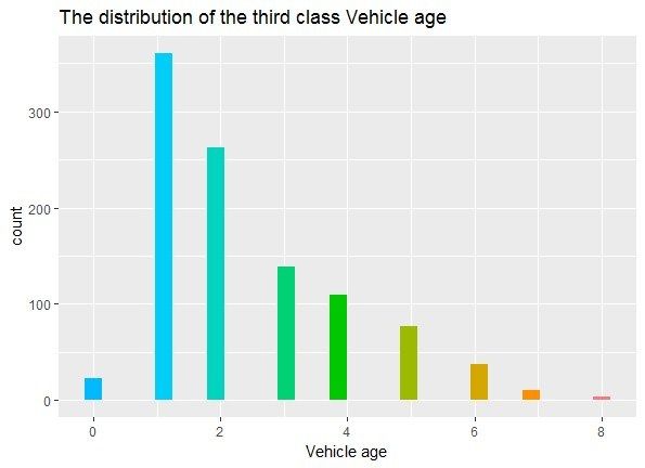
Int. J. Financial Stud. 2018, 6, 18 7 of 16
Int. J. Financial Stud. 2018, 6, x FOR PEER REVIEW 7 of 16
Int. J. Financial Stud. 2018, 6, x FOR PEER REVIEW 7 of 16
Figure 3. Distribution of owners’ age.
Figure 3. Distribution of owners’ age.
As shown in Figure 3, the first class of owners’ age is centrally distributed between 39 and 51
As shown
years in second
old, the Figureclass
3, the Figure
first
is centrally 3.
class Distribution
of owners’
distributed of owners’
age is25age.
between centrally distributed
and 53 years between
old, the third class 39
is and
51 years old, the
centrally second between
distributed class is centrally
23 and 55distributed
years old. between
In case of25the and 53 yearsresult,
clustering old, the third
there class is
is no
As shown in Figure 3, the first class of owners’ age is centrally distributed between 39 and 51
significant
centrally relationships
distributed between between
23 andthe55owners’
years old.ageInand theof
case risk
theclassification. By experience,
clustering result, there is noyounger
significant
years old, the second class is centrally distributed between 25 and 53 years old, the third class is
drivers are more likely
relationships to have accidents due risk
to lack of driving experiences but drivers of this age are
centrally between
distributedthebetween
owners’ 23age
andand
55 the classification.
years old. In case of the By clustering
experience, younger
result, there drivers
is no
group have
moresignificant higher
likely to have physical
accidents quality
due to and relatively high response ability.
relationships between thelack of driving
owners’ age andexperiences but drivers
the risk classification. of this ageyounger
By experience, group have
higher physical
drivers quality
are more andtorelatively
likely high due
have accidents response
to lackability.
of driving experiences but drivers of this age
4.2.3. Auto Age
group have higher physical quality and relatively high response ability.
4.2.3. Auto Age
According to the classification of the auto age, the results are shown in Table 2 and the
distribution
4.2.3. of auto age is presented in Figure 4.
Auto Age
According to the classification of the auto age, the results are shown in Table 2 and the distribution
According
of auto age to the
is presented in classification
Figure 4. Tableof 2.the auto age, ofthe
Classification results
auto age. are shown in Table 2 and the
distribution of auto age is presented in Figure 4.
Auto Age (Years) 0 1 2 3 4 5 6 7 8 9 10 10 or more
The First Category
Table 2. Classification
24 145 118 86 61
of auto age.
39 33 15 7 6 2 0
Table 2. Classification of auto age.
The Second Category 17 370 283 212 118 72 43 27 22 22 19 19
Auto Age
The (Years)
Third
Auto (Years) 0
AgeCategory 0 1 361
23 1 2 2632 3 139
3 41094 577
5 66 11
37 7 7 84 890 09
10 10 10 10 or more
or0more
The FirstThe
Category 24
First Category 145 145118 118 86 86 6161 39
24 39 33 15 15 7 76
33 26 20 0
The Second
The Category 17
Second Category 370 370283 283212212 118
17 118 72
72 43 27 27 22 22
43 22 22
19 1919 19
The Third
The Category 23
Third Category 361 361263 263139139 109
23 109 77
77 37 11 11 4 40
37 00 00 0
Figure 4. Cont.Int. J. Financial Stud. 2018, 6, 18 8 of 16
Int. J. Financial Stud. 2018, 6, x FOR PEER REVIEW 8 of 16
Figure 4. Distribution of auto age.
Figure 4. Distribution of auto age.
According to the high-risk definition of the first class, the auto age of the second class is
According
concentratedto the years
in 1–3 high-risk definition
but autos of the
that are older first
than class,old
10 years theareauto
all inage of theThe
this class. second class is
auto ages
concentrated in 1–3
of the third classyears but autos that
are concentrated areyears
in 1–3 olderold,
than 10 years
which meansoldtheare all in
autos arethis
in aclass.
goodThe auto ages
situation
of thewith noclass
third elderare
ones.
concentrated in 1–3 years old, which means the autos are in a good situation with
Therefore, the determination of the risk based on auto age still needs further validation.
no elder ones.
Therefore, the determination of the risk based on auto age still needs further validation.
4.2.4. Claim Frequency
4.2.4. Claim Frequency
According to the classification, the results are shown in Table 3.
According to the classification, the results are shown in Table 3.
Table 3. Distribution of claim frequency in three classes.
Claims
Table 3.Frequency
Distribution−3 −2 frequency
of claim −1 1 in three
2 3classes.
4 5
The First Class 31 57 152 271 0 20 3 2
Claims Frequency The Second−3Class −2211 212 −1 412 1 388 0 2 1 0 3 0 4 5
The First Class The Third31Class 57 86 111
152 284271490 0 0 40 9 204 3 2
The Second Class 211 212 412 388 0 1 0 0
From
TheTable
Third3,Class
it can be seen
86 clearly111
that the284
claim frequency
490 0under 0 40
in the second
9 and4 third
classes hold a higher proportion, which is consistent with the lower signed premium in the second
and third class. The claim frequency under 0 in the first class holds a lower proportion, which is
From Table 3, it can be seen clearly that the claim frequency under 0 in the second and third
consistent with the higher signed premium in the first class.
classes hold a higher proportion, which is consistent with the lower signed premium in the second and
third 4.2.5.
class.The
TheEconomic
claim frequency under
Significance 0 in the first class holds a lower proportion, which is consistent
of Variables
with the higher signed premium in the first class.
The economic significance of variables in the model are as follows:
4.2.5.(1)
TheThere is certain
Economic reference value
Significance of the auto burden index for the vehicle insurance rate. Through
of Variables
the clustering results, it is suggested that insurance companies could predict the premiums of
The economic
the insuredsignificance of variables
by introducing the auto in the model
burden indexare asthe
into follows:
model. In the empirical study,
the autos with a higher burden index ware charged with a relatively high premium. Therefore,
(1) There is certain reference value of the auto burden index for the vehicle insurance rate. Through
insurance companies could divide them into high-risk class, especially the autos with auto
the clustering results, it is suggested that insurance companies could predict the premiums of the
burden index more than 20 deserve more attention.
insured
(2) Based byonintroducing
the clusteringthe autoof
results burden index
owners’ intoauto
age and theage,
model. In the empirical
it is suggested that the study, theofautos
influence
withdriving
a higher burden index ware charged with a relatively high premium. Therefore,
experience should be considered in the evaluation of the auto owners by insurance insurance
companies
companies.could
Anddivide them
the auto withinto high-risk
a younger class,
age is especially
supposed to have the autos
a good with auto
condition, burden
which helpsindex
moretothan
safe 20 deserve
driving. more attention.
However, according to the above results, the influence of auto age on risks
(2) Basedshould be discussed
on the clusteringinresults
more details. Autos with
of owners’ goodauto
age and conditions
age, ithave a large proportion
is suggested that theininfluence
the
first high-risk class. Studies have shown that most auto accidents are caused
of driving experience should be considered in the evaluation of the auto owners by insurance by human factors.
This view also confirms the clustering results of auto age. However, for autos over 10 years of
companies. And the auto with a younger age is supposed to have a good condition, which helps
age, further discussion and analysis are still needed in the insurance process.
to safe driving. However, according to the above results, the influence of auto age on risks should
(3) After the reform of commercial auto insurance in Chongqing in 2015, non-claiming benefits will
be discussed
be taken intoin more
account details. Autos
in the auto with good
insurance conditions
rate, which meanshave a large with
that persons proportion in the first
fewer insured
high-risk class. Studies have shown that most auto accidents are caused by human factors. This
view also confirms the clustering results of auto age. However, for autos over 10 years of age,
further discussion and analysis are still needed in the insurance process.Int. J. Financial Stud. 2018, 6, 18 9 of 16
(3) After the reform of commercial auto insurance in Chongqing in 2015, non-claiming benefits will
be taken into account in the auto insurance rate, which means that persons with fewer insured in
the past are supposed to pay lower premiums. In the first high-risk class, the claims frequency of
policyholders is relatively high, along with an increase in the risk, wherefore it is reasonable for
the insurance company to charge higher premiums.
5. Selection of the Loss Distribution
It’s difficult to construct the empirical distribution of the insured for quantitative analysis, so that
the use of loss distribution is a better alternative, which requires selecting the appropriate distribution
among several loss distributions. This section is implemented using the GENMOD program in SAS
software. In this article, two different distributions are used to figure out the correlation of claim
frequency and variables, claim cost and variables. We use the Poisson distribution and the negative
binomial distribution to fit the claim frequency in case it follows a discrete distribution. We use
the Gamma distribution and Inverse Gaussian distribution to fit the claim cost in case it follows a
continuous distribution. According to the canonical form of the link function, we use the logarithm
function, the logit function and the identity function respectively in the Gamma distribution and the
Poisson distribution, the negative binomial distribution and the Inverse Gaussian distribution.
The formula of the claims cost is as follows, indicating an opposite relationship between the claim
cost and the claim frequency.
L
S=
N
S is the claimscost, L for the losses and N is the claim frequency. The average loss per claim
intensity can be based on net loss, excluding various loss-adjusted costs, as well as assessed or total
loss-adjusted costs, which can be paid, incurred, or predicted final losses. The claim could be the
number of final claims that have been reported, paid, closed or predicted.
5.1. Loss Distribution of Claim Frequency
For non-life insurance business, the distribution of individual insurance claims frequency is
uncertain. The claims frequency can be described as a random variable, which can be described by
its probability distribution. The theoretical distributions of claims frequency are Poisson distribution,
binomial distribution and negative binomial distribution.
The Poisson distribution and the negative Binomial distribution are commonly used to fit the
claim frequency since it is a non-negative discrete variable. In the context of actuarial literature,
Denuit and Lang (2004), Yip and Yau (2005) and others proposed the extracted reference from the
Poisson distribution, which is used as the main method to estimate the claim frequency. The negative
binomial distribution is used as a functional form to relax the restriction of equidispersion in the Poisson
model. The literature presents many of the ways to construct the negative binomial distribution but
Boucher et al. (2008) argue that the more intuitive one is the introduction of a random heterogeneity
term of mean 1 and Variance in the mean parameter of the Poisson distribution. This general approach
is discussed at length by Winkelmann (2004) and Greene (2008) and so on. Regarding the usage of the
insurance data, a classic example arises from the theory of accident proneness which was developed
by Greenwood and Yule (1920).This theory sustains that the number of accidents follows the Poisson
distribution but there is Gamma-distributed unobserved individual heterogeneity, reflecting the fact
that the true mean is not perfectly observed. The distribution function of the Poisson distribution can
be expressed as:
exp(−λi )λi yi
Pr (Yi = yi ) =
yi !
The probability density function of the negative binomial distribution is:
Γ ( α + yi ) α α λi
Pr (Yi = yi ) = ( ) ( )
Γ ( α ) Γ (1 + y i ) α + y i λi + αInt. J. Financial Stud. 2018, 6, 18 10 of 16
( λ )2
The mean and variance of the negative binomial distribution is E(Yi ) = λi and Var (Yi ) = λi + αi .
According to the relationship between the mean and variance, the negative binomial distribution is the
more over-dispersed with a smaller α. When α → ∞, the negative Binomial distribution is degenerated
into Poisson distribution. According to the factors of ratemaking used by the China Insurance Industry
Association, we made a classification of the owners’ ages, the auto burden index, the driving areas in
Chongqing, auto age, the claim frequency and the claim cost, Five levels are divided according to the
above indicators, as shown in Table 4. (unit: thousand).
Table 4. Rate factor grading table (Yu represents Chongqing in China).
Level Factor 1 2 3 4 5
Owners Age [20, 30) [30, 40) [40, 50) [50,60) [60, 70)
Auto burden index [0, 10) [10, 15) [15, 20) [20, ∞)
Area Yu A Yu B Yu C Yu F Yu G
Auto age [0, 90) [90, 360) [360, 1080) [1080, 1800) [1800, ∞)
Claim cost [0, 1) [1, 3) [3, 8) [8, 15) [15, ∞)
According to Table 5, the claim frequency is negatively correlated with the owner’s age and the
auto age, the physiological status and psychological state of the auto owners are closely related to their
ages. Generally, young people are more aggressive. Although older drivers are more prudent because
of their rich driving experience, their physiology will gradually recess as age increases. As a result,
older drivers have much slower emergency response than young people, so that both young and
old drivers belong to the group with high accident rates. The coefficients of auto burden index and
driving areas did not pass the significance test in the two distributions, so that they require to be
further analyzed. David and Jemna (2015) fitted the claim frequency with the Poisson distribution
and the Negative Binomial distribution respectively, they pointed out that the Negative Binomial
distribution fitted claim frequency better than the Poisson distribution. According to the fitting
results of the Poisson and negative binomial distributions of the claim frequency, the p-value of the
estimated parameters in Poisson distribution is obviously smaller than that of the negative binomial
distribution, indicating that the fitting result of Poisson distribution is relatively better. Based on the
data in this article, we found that the Poisson distribution has a better fitting effect than the Negative
Binomial distribution.
Table 5. The claim frequency fitted by two distributions.
Poisson Distribution Negative Binomial Distribution
Factors Level
Coefficient p Value Coefficient p Value
Intercept −6.4953 0.0168 −7.8303 0.0133
Owners age 1 −2.7985 0.0493 −1.6278 0.0701
Owners age 2 −2.4399 0.054 −1.3198 0.0756
Owners age 3 −5.3297 0.0181 −2.6768 0.0528
Owners age 4 −2.5146 0.0543 −1.7192 0.0679
Owners age 5 0.0000 0.0000
Auto burden index 1 −0.2658 0.2074 −0.0747 0.7611
Auto burden index 2 0.1331 0.4598 0.0166 0.9361
Auto burden index 3 0.2362 0.2429 0.0785 0.7361
Auto burden index 4 0.0000 0.0000
Area 1 −0.18 0.3413 −0.0786 0.7167
Area 2 0.0796 0.7105 0.0354 0.8835
Area 3 0.1777 0.3848 0.0616 0.7914
Area 4 0.3751 0.0891 0.1784 0.4749
Area 5 0.0000 0.0000
Auto age(days) 1 −0.2635 0.0339 −0.1023 0.0730
Auto age 2 −0.7033 0.0004 −0.3378 0.1268
Auto age 3 −0.6578 0.0012 −0.3744 0.0957
Auto age 4 −0.6935 0.0006 −0.3980 0.0713
Auto age 5 0.0000 0.0000Int. J. Financial Stud. 2018, 6, 18 11 of 16
5.2. Loss Distribution of Claim Cost
Since the claim costs usually follow a negatively skewed distribution, they are usually fitted by
the Gamma distribution and the Inverse Gaussian distribution. The probability density function of the
Gamma distribution can be expressed as:
v
1 yi v yi v
f ( yi ) = exp(− )
yi Γ ( v ) µ µ
The probability density function of the Gamma distribution is negatively skewed and its variance
equals to the square of the mean. The probability density function of the Inverse Gaussian distribution
can be expressed as:
λ 1 yi − µ 2
f ( yi ) = p exp[− ( ) ]
σ 2πyi 3 2yi µσ
The probability density function of the Inverse Gaussian distribution is also negatively skewed
and its variance equals to the cubic of the mean. Given the mean and variance, the Inverse Gaussian
distribution belongs to the right partial thick tail distribution and its tail is thicker than the Gamma
distribution. The following is the fitting result of the claim costs:
From Table 6 we can see that the claims costs are positively correlated with owners’ age and auto
age. In the case of the loss, the strength of the claim is inversely proportional to the number of claims,
so that the older drivers have lower claims.
Table 6. The claim cost fitted by two distributions.
Inverse Gaussian Distribution Gamma Distribution
Factors Level
Coefficient p Value Coefficient p Value
Intercept 2.2706 0.0003 2.2157 0.0001
Owners Age 1 5.5980 0.0296 5.9243 0.0220
Owners Age 2 5.5574 0.0276 6.0388 0.0194
Owners Age 3 5.2173 0.0303 5.7490 0.0213
Owners Age 4 1.5209 0.0773 2.2316 0.0642
Owners Age 5 0.0000 0.0000
Auto burden index 1 −0.3459 0.2612 −0.2936 0.2803
Auto burden index 2 −0.0495 0.8558 −0.0531 0.8232
Auto burden index 3 −0.2873 0.3318 −0.2500 0.3401
Auto burden index 4 0.0000 0.0000
Area 1 0.2892 0.2378 0.2716 0.2338
Area 2 0.2548 0.3578 0.2130 0.4080
Area 3 0.3120 0.2437 0.2592 0.2973
Area 4 0.4862 0.1197 0.4289 0.1275
Area 5 0.0000 0.0000
Auto Age 1 0.2850 0.0586 0.3178 0.0458
Auto Age 2 0.3850 0.0025 0.3489 0.0022
Auto Age 3 0.0974 0.0777 0.0921 0.0753
Auto Age 4 0.3852 0.0004 0.3609 0.0002
Auto Age 5 0.0000 0.0000
But the coefficients of auto burden index and driving areas did not pass the significance test in
the two distributions, which requires to be further analyzed. Mihaela David (2015) used the Gamma
distribution to fit the claim costs and its influencing factors. Judging from the fitting results of the
inverse Gaussian distribution and Gamma distribution, most p-values of parameter estimation in
Gamma distribution are smaller than that of the inverse Gaussian distribution, indicating that the
fitting result of Gamma distribution is relatively better. Therefore, based on the data in this paper, it is
more advisable to use the Gamma distribution to fit claims cost than the inverse Gaussian distribution.Int. J. Financial Stud. 2018, 6, 18 12 of 16
6. Generalized Linear Model
The hypothesis of generalized linear model includes random component, system component and
link function. The formulas are as follows:
E(Yi ) = µi = g−1 (∑ Xij β j )
ΦVar (µi )
Var (Yi ) = ωi
Random component is the probability distribution of the dependent variable or error term. Each
observation Yi of the dependent variable Y is independent from each other, following a distribution in
the exponential distribution family, 1 as the Poisson distribution, the Inverse Gaussian distribution
and the Gamma distribution. The model is expressed as follows:
( yi ) − b ( θi )
f (yi ; θi ; Φ) = exp + c ( yi , Φ )
α(Φ)
where α(φ) >0 and α(φ) is a continuous function usually in the form of, ω is the priori weight. φ is the
(y )−b(θ )
discrete parameter, which is the variance of y. The first and second derivatives of i α(Φ) i exist and
are more than 0.
c(yi ,φ) is a function of the observed value and the discrete parameter, which is independent of
the parameter θ i . The system component is a linear combination of independent variables, which is
expressed as:
η i = Xi β
The link function establishes a specific relationship between the random component and the
system component:
E(Yi ) = µi = g−1 (η i )
where g(µi ) is the link function to link X and E(Y), expanding the application range of the generalized
linear models. McCullagh and Nelder (1989) summarized the form of link functions in generalized
linear models. In the study of auto insurance ratemaking models, the logarithmic link and the logit link
function are the most commonly used functions. The logarithmic link function ensures the predicted
value of the variables to be non-negative, while logit link function ensures the predicted value of
the variables to be between [0, 1]. The Logistic regression was first proposed by P. F. Verhulst in
1838. Comparing with linear regression, the advantages of Logistic regression are as follows: first,
when the dependent variables are discrete, Logistic regression can avoid heteroscedasticity. Second,
the Logistic regression model does not require strict assumption son the sample data or require the
variables to follow the Normal distribution. Third, it’s possible to take a wider range of dependent
variables into account to enhance the significance of the model. Let X = (x1 ,...,xr ) be a factor that
affects an event, y represents dichotomous variables indicating an accident whether occurs or not.
y equals to 1 if the event occurs and 0 otherwise. In the model, themean can be expressed as
p
E(Yi ) = µi = exp x T β /1 + exp x T β = g−1 (ηi ) and g(µi ) = ln 1− p is the link function which
p
transforms η into the probability of occurrence p. The transformation is called the logit transform. 1− p
is called the odds ratio, indicating the probability of a relative occurrence. p represents the probability
p
of the event occurrence, while 1− p representing the ratio of the probability of the two cases, which is
p
called the odds ratio. The logarithm of 1− p is called the log it transformation of p. It can be expressed as:
p( x ) r
log it( p) = ln 1− p = β0 + ∑ β j (x j )
i =1
p( x ) = Pr (y = 1| x )Int. J. Financial Stud. 2018, 6, 18 13 of 16
(x1 ,...,xr ) is the dependent variables, βj is the regression coefficient of xj . Take the index on both sides
of the above formula, p can be expressed as:
e β0 + β1 x1 +...+ βr
p = E ( y = 1| x1 , x2 , . . . , xr ) =
1 + e β0 + β1 x1 +...+ βr
This is the basic form of the Logistic model. In this article, y is equals to 1 if the event occurs and 0
otherwise, p denotes the probability that the policy will be claimed. Adriana Bruscato Bortoluzzo (2011)
pointed out that the claim probability is more convincing than the claim size. Therefore, this article
uses the Logistic Regression model to predict the claim probability.
After establishing the Logistic regression model, it is necessary to assess the validity of the model.
The main criteria are Pearson χ2 , Deviance, AIC and Schwartz criteria (SC). Pearson and Deviance
statistics follow the χ2 distribution, AIC and SC are the statistics that compares different settings of the
models. Different models can be sorted according to their AIC and SC index values, the model with a
smaller AIC and SC are considered to be better.
The AIC and BIC statistics of the claim strength prediction model are respectively expressed as:
AIC = L(θ ) + 2k
BIC = L(θ ) + k ln n
where K is the number of parameters in the model, n is the sample size. The smaller the number of
AIC and BIC, the better the model is.
In Tables 5 and 6, the coefficients of auto burden index and the driving areas did not pass the
significance test, its necessary to adjust the variables before the Logistic regression. Since the factor
driving areas are discrete variables with six values, we split the factor into six variables: Area.a, Area.b,
Area.c, Area.f, Area.g and Area.other, as dummy variables. Area.a is taken as 0, which is supposed to
be a reference to all variables. Since many insurers tend to give some concessions to the insured who
had not claimed last year and raise the premiums of the insured who had more claims last year, we split
the claim frequency into 6 variables: Frequency-2, Frequency-1, Frequency1, Frequency3, Frequency4
and Frequency5, corresponding to the insured who had not claimed last two years, the insured who
had not claimed last year, the insured who had claimed 1–2 times, the insured who had claimed
3 times, the insured who had claimed 4 times and the insured who had claimed 5 times respectively.
The results are as follows in Table 7:
Table 7. The Logistic regression regardless of the auto burden index.
Variable Variable Description Estimate Std. Error Z Value Pr (>|Z|)
Intercept Constant −1.16545492 0.098102707 −11.87994656 1.50 × 10⁻³²
Age Age 0.00085517 0.00178175 0.479961092 0.631255059
Area.b YuB −0.081976692 0.052954976 −1.548045139 0.121611429
Area.c YuC −0.644885609 0.041216826 −15.64617346 3.53 × 10−55
Area.f YuF −0.303218184 0.049630575 −6.109503751 9.99 × 10⁻¹⁰
Area.g YuG −0.722177901 0.061717256 −11.70139361 1.25 × 10⁻³¹
Area.other Other provinces −0.389089035 0.12354669 −3.149327871 0.001636465
Duration Car age −0.116197532 0.007479984 −15.53446254 2.03 × 10−54
Frequency-2 Two years without claim 0.238596945 0.067859735 3.516031219 0.00043805
Frequency-1 No claim last year 0.434567151 0.06083322 7.143582905 9.09 × 10⁻¹³
Frequency1 1 or 2 claims 0.788715004 0.05687611 13.86724585 1.00 × 10−43
Frequency3 3 claims 1.41202745 0.117971645 11.96921049 5.15 × 10⁻³³
Frequency4 4 claims 1.551668395 0.250396246 6.196851676 5.76 × 10⁻¹⁰
Frequency5 5 claims 2.289320564 0.380331911 6.019270272 1.75 × 10⁻⁹
Null deviance: 25,250 on 24,405 degrees of freedom, Residual deviance: 24,046 on 24,392 degrees of freedom, p
value of Residual deviance: 0.9419055 AIC: 24,074 data volume: 24,407.
The deviance statistic of the model approximately follows the Chi-square distribution with
n–p degrees of freedom and is used to the significance test of the model. As seen from the results,Int. J. Financial Stud. 2018, 6, 18 14 of 16
the p-value of the model approximately equals to 0.94 but it is far more than 0.05 or 0.1, indicating that
the fitting effect is very good and the deviance test could not deny the hypothesis of the model.
From the analysis of the regional factors, the coefficients of the main urban areas are negative,
indicating that the autos belonging to the main urban areas have an increased probability of claims.
The greater the absolute value of the area coefficients, the lower the probability of the claims in the
area, compared to the main urban area. The longer the auto age, the lower the probability of claims.
The coefficients of the claim frequency are all positive, in case that the reference is the variable which
had no claim in the last three years, indicating that the probability of claims rises as the claim frequency
increases. From the perspective of the odds ratio, comparing frequency 1 with the reference variable,
it’s clear that the probability of claim increased 120% when there was a claim last year. Under the
same conditions, the probability of claim increased 310.4% .When there were 3 claims last year. As it
can be seen, the influence of claim frequency on the claim probability is significant. In the cluster
analysis, we have analyzed the relationship between the auto burden index, the settled amount and
the total signed premium, more than 80% of the autos with the auto burden index greater than 20 are
concentrated in the first high-risk class. Therefore, the variable auto burden index is introduced into
the Logistic regression model. The results are as follows in Table 8:
Table 8. Results of the Logistic regression model considering the auto burden index.
Variable Variable Description Estimate Std. Error Z Value Pr (>|Z|)
Intercept Constant −6.894 × 10⁻¹ 3.084 × 10⁻¹ −2.236 0.025371
Owners age Age −6.612 × 10⁻³ 4.783 × 10⁻³ −1.382 0.166881
Area.b YuB −1.166 × 10⁻¹ 1.338 × 10⁻¹ −0.872 0.383177
Area.c YuC −4.221 × 10⁻¹ 1.123 × 10⁻¹ −3.757 0.000172
Area.f YuF −2.271 × 10⁻¹ 1.423 × 10⁻¹ −1.596 0.110486
Area.g YuG −4.874 × 10⁻¹ 1.588 × 10⁻¹ −3.070 0.002141
Area.other Other provinces −5.018 × 10⁻¹ 3.305 × 10⁻¹ −1.518 0.128919
Auto age Car age −2.060 × 10⁻⁴ 6.585 × 10⁻⁵ −3.129 0.001755
Auto burden index Burden index −5.179 × 10⁻³ 1.015 × 10⁻² −0.510 0.609947
Frequency-2 Two years without claim 1.280 × 10⁻¹ 1.959 × 10⁻¹ 0.654 0.513395
Frequency-1 No claim last year 3.979 × 10⁻¹ 1.742 × 10⁻¹ 2.284 0.022377
Frequency1 1 or 2 claims 7.966 × 10⁻¹ 1.638 × 10⁻¹ 4.863 1.16 × 10⁻⁶
Frequency3 3 claims 1.062 3.016 × 10⁻¹ 3.521 0.000430
Frequency4 4 claims 1.973 6.342 × 10⁻¹ 3.110 0.001869
Frequency5 5 claims 2.011 8.832 × 10⁻¹ 2.277 0.022788
Null deviance: 3353.9 on 2783 degrees of freedom, Residual deviance: 3250.6 on 2769 degrees of freedom, p value of
Residual deviance: 4.146477 × 10⁻¹⁰ AIC: 3280.6 data volume: 2783.
Although the model considering the auto burden index could not well estimate the probability
of claims, it is due to the lack of validity in the data. If a better data is used, a better result could
be carried out. The insurance company could assess the risk of the insured according to this claim
probability model.
7. Conclusions
This article aims to show that it is necessary to consider the auto burden index into the traditional
rate making model. It is recommended that insurance companies take the burden index as an important
factor to determine the model.
In this article, the Logistic regression model is used to fit the insurance data of an insurance
company in China. On the basis of summarizing relevant literature, the theoretical analysis and
empirical analysis were carried out by cluster analysis, fitting of loss distribution and Logistic
regression model. According to the fitting effect of the loss distribution, the Poisson distribution
should be used to fit the claim frequency and the Gamma distribution should be used to fit the claim
cost. After adding the dummy variables to replace the original variables which are not significant,
most of the new variables passed the significance test, indicating that the driving areas and the claimInt. J. Financial Stud. 2018, 6, 18 15 of 16
frequency have a significant correlation with the probability of claims. Based on the AIC criteria,
the AIC of the model considering the auto burden index was reduced significantly from 24,074 to
3280.6. Therefore, the model considering auto burden index has a good fitting effect in auto insurance
rate-making. This model assumes that the factors are independent of each other and the cross-effects
between the factors were not taken into account, a better result could be attained if the cross-factors is
considered. In the analysis, the limitation of data sources also affects the Logistic regression results and
the significance of the coefficients. From the perspective of the fitting effect of the model considering
the auto burden index, the coefficient of the auto burden index is not significant in the model, we
speculated that it is due to the lack accuracy of the auto burden index in current evaluation and there
is not a uniform caliber for many indicators.
Most of the data volume of current insurance company did not reach the requirements of the
generalized linear models, leading to the homogeneity of the policy and the lack of information of
the owners. The higher the homogeneity of the policy, the greater amount of the data required to
refine the classification of risk factors. The lack of owners’ information may lead to the neglect of
some new variables, which may have little influence on the model and could not pass the significance
test. With the development of the socio-economic, some non-significant variables may transform
into significant variables. Therefore, it is necessary to establish a uniform database for the insurance
company to provide a benchmark for auto insurance rate-making. In addition, the generalized linear
models have become the main method of auto insurance rate-making. With its simple operation and
strong feasibility, it is popular with property insurance companies. It also takes a certain amount of
time to make it extensively used, especially the lack of technical means of the model diagnosis, which
is the focus of the research in the future.
Author Contributions: Zhengmin Duan, as the guidance teacher, whole-process guidance. Yonglian Chang,
Qi Wang participated in model establishment, the Chinese and English articles editor, and later post revision
work. Qing Zhao and Tianyao Chen participated in the model establishment.
Conflicts of Interest: The authors declare no conflicts of interest.
References
Aitkin, M., D. Anderson, B. Francis, and J. Hinder. 1989. Statistical Modeling in GLM. Oxford: Oxford University Press.
Anderson, Duncan, Sholom Feldblum, Claudine Modlin, Doris Schirmacher, Ernesto Schirmacher, and Neeza Thandi.
2004. A Practitioners Guide to Generalized Linear Models, 3rd ed. Arlington: Casualty Actuarial Society, Discussion
Paper Program, pp. 1–116.
Bailey, Robert A. 1963. Insurance Rates with Minimum Bias. Arlington County: Casualty Actuarial Society.
Bailey, Robert A., and LeRoy J. Simon. 1960. Two studies in automobile insurance ratemaking. Astin Bulletin
1: 192–217. [CrossRef]
Bortoluzzo, Adriana Bruscato. 2011. Estimating Total Claim Size in the Auto Insurance Industry: A Comparison
between Tweedie and Zero-Adjusted In-verse Gaussian Distribution. BAR-Brazilian Administration Review
8: 37–47. [CrossRef]
Boucher, Jean-Philippe, Michel Denuit, and Montserrat Guillen. 2008. Models of Insurance Claim Counts with Time
Dependence Based on Generalization of Poisson and Negative Binomial Distributions. Variance 2: 135–62.
Cheng, Zhenyuan. 2007. Research on Asymmetric Information in Insurance Market. Beijing: People’s Publishing
House, pp. 65–82.
Crocker, Keith J., and Arthur Snow. 1986. The Efficiency Effects of Categorical Discrimination in the Insurance
Industry. Journal of Political Economy 94: 321–44. [CrossRef]
David, Mihaela. 2015. Auto insurance premium calculation using generalized linear Models. Procedia Economics
and Finance 20: 147–56. [CrossRef]
David, Mihaela, and Dănuţ-Vasile Jemna. 2015. Modeling the frequency of auto insurance claims by means of
poisson and negative binomial models. Annals of the Alexandru Ioan Cuza University-Economics 62: 151–68.
[CrossRef]
Denuit, Michel, and Stefan Lang. 2004. Nonlife ratemaking with Bayesian GAMs. Insurance: Mathematics and
Economics 35: 627–47. [CrossRef]You can also read