Geographically varying relationships of COVID 19 mortality with different factors in India - Nature
←
→
Page content transcription
If your browser does not render page correctly, please read the page content below
www.nature.com/scientificreports
OPEN Geographically varying
relationships of COVID‑19
mortality with different factors
in India
Asif Iqbal Middya & Sarbani Roy *
COVID-19 is a global crisis where India is going to be one of the most heavily affected countries.
The variability in the distribution of COVID-19-related health outcomes might be related to many
underlying variables, including demographic, socioeconomic, or environmental pollution related
factors. The global and local models can be utilized to explore such relations. In this study, ordinary
least square (global) and geographically weighted regression (local) methods are employed to
explore the geographical relationships between COVID-19 deaths and different driving factors. It is
also investigated whether geographical heterogeneity exists in the relationships. More specifically,
in this paper, the geographical pattern of COVID-19 deaths and its relationships with different
potential driving factors in India are investigated and analysed. Here, better knowledge and insights
into geographical targeting of intervention against the COVID-19 pandemic can be generated by
investigating the heterogeneity of spatial relationships. The results show that the local method
(geographically weighted regression) generates better performance (R2 = 0.97) with smaller Akaike
Information Criterion (AICc = −66.42) as compared to the global method (ordinary least square). The
GWR method also comes up with lower spatial autocorrelation (Moran’s I = −0.0395 and p < 0.01)
in the residuals. It is found that more than 86% of local R2 values are larger than 0.60 and almost
68% of R2 values are within the range 0.80–0.97. Moreover, some interesting local variations in the
relationships are also found.
The novel coronavirus disease (COVID-19) has spread rapidly to all parts of the world, causing almost 2.5 mil-
lion deaths as of mid-February 2 0211. Because of its unpredictable nature and lack of appropriate medications,
COVID-19 is now a global health concern. There is unprecedented urgency to investigate the major factors that
are related to COVID-19 death. In this context, recent studies are focusing on exploring person-specific risk
factors for COVID-19-related health o utcomes2–4. Also, there are research works that examine the association of
COVID-19-related health outcomes with different socio-economic, environmental, and region-specific factors5–7.
These factors play a very important role in determining the patterns of COVID-19 mortality.
Both global and local models can be utilized to explore the above-mentioned associations. A global model
comes up with a geographically constant relationship across the entire geographic space. On the other hand, a
local model can capture the local relationships that can vary across the geographic space. Most of the studies
that focus on exploring the relationship of COVID-19 cases with different possible risk factors are based on
global models (e.g. Ordinary Least Square)8,9. But, the global models assume that the associations between the
independent variables and the dependent variable are stationary (i.e. homogeneous) throughout the study area.
Besides, these models also assume that there is no spatial autocorrelation in the dataset. Eventually, they yield
ehaviour10. But, in reality, the relationships between the depend-
estimates of the parameters that reflect average b
ent and the independent variables may not be homogeneous and can be geographically v arying11. Therefore, such
models usually suffer from low accuracy especially in those locations where weak association exists between
dependent and independent variables. Now, various local techniques can be utilized in order to overcome the
above-mentioned shortcomings of the global models. Some widely encountered local spatial statistics include
geographically weighted regression (GWR)12,13, local Moran’s I14, spatial regressions, etc.
As of 24 February 2021, India is the world’s second worst-affected country by COVID-19, with a total number
of deaths exceeding 156.7 thousand and a total number of confirmed cases exceeding 11 m illion1. However, in
Department of Computer Science and Engineering, Jadavpur University, Kolkata 700032, India. *email: sarbani.
roy@jadavpuruniversity.in
Scientific Reports | (2021) 11:7890 | https://doi.org/10.1038/s41598-021-86987-5 1
Vol.:(0123456789)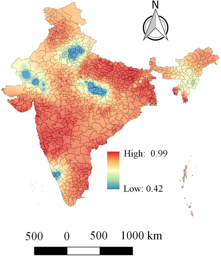
www.nature.com/scientificreports/
Figure 1. Geographical distribution of COVID-19 deaths across India. The spatially continuous distribution
map is generated in QGIS (https://qgis.org/en/site/) by using Inverse Distance Weighting (IDW) interpolation.
India, no comprehensive study is performed at the local level to investigate geographical relationships between
COVID-19 deaths and associated potential factors. To bridge the gap, a local method (GWR) is employed to
explore the geographical distribution and associated potential socio-economic, demographic, and environmental
factors for COVID-19 deaths. Note that, the GWR model helps us to identify whether there is geographical het-
erogeneity present in the relationships. Moreover, a comparison between local (OLS) and global (GWR) models
are also performed. This paper offers further knowledge and insight into geographical targeting of intervention
and control strategies against the COVID-19 epidemic. In summary, the key objectives of this study are (i) to
explore the potential socio-economic, demographic, and environmental driving factors for COVID-19 deaths
in India; (ii) to investigate geographically varying relationships of COVID-19 deaths with the driving factors
by employing local (GWR) model. (iii) comparing the results of the local (GWR) model with the global (OLS)
model to validate its suitability.
Materials and methods
Data description. The geographical variabilities of COVID-19 deaths are modeled based on the district-
level data across India. Note that, the COVID-19 mortality data are acquired for more than 400 districts in India.
The geographical distributions of COVID-19 deaths are shown in Fig. 1. The largest number of COVID-19
deaths are observed in the districts of the state Maharashtra. A total of 9 among 28 states contains at least one
district that reports more than 1000 COVID-19 deaths. Table 1 summarizes all the raw datasets, their descrip-
tions, the sources including the links from where these data can be found, and potential factors (independent
variables) that are extracted from the raw datasets.
Datasets. Three raw datasets are mainly utilized to investigate geographically varying relationships of COVID-
19 deaths with different environmental, demographic, and socio-economic factors. The first dataset includes
district wise COVID-19 death counts in India. The cumulative number of COVID-19-related deaths for each
district is collected up to February 24, 2021, from the COVID19INDIA website (https://www.covid19india.
org/). COVID19INDIA is a crowdsourced initiative to document the COVID-19 data from the states and union
territories of India. In this study, the district-level COVID-19 death count is considered as the dependent vari-
able. The second dataset pertaining to environmental pollution includes the daily concentration of different air
pollutants (e.g. PM2.5, SO2, NO2, etc.). The concentration of air pollutants (from January 2016 to January 2020)
for a total of 130 monitoring stations are obtained from the Central Pollution Control Board ( CPCB15), INDIA.
The third dataset contains socio-economic and demographic data that may have an association with COVID-19
mortality. The district-level socio-economic and demographic data are obtained from the last census in India
that was conducted in 2011.
Scientific Reports | (2021) 11:7890 | https://doi.org/10.1038/s41598-021-86987-5 2
Vol:.(1234567890)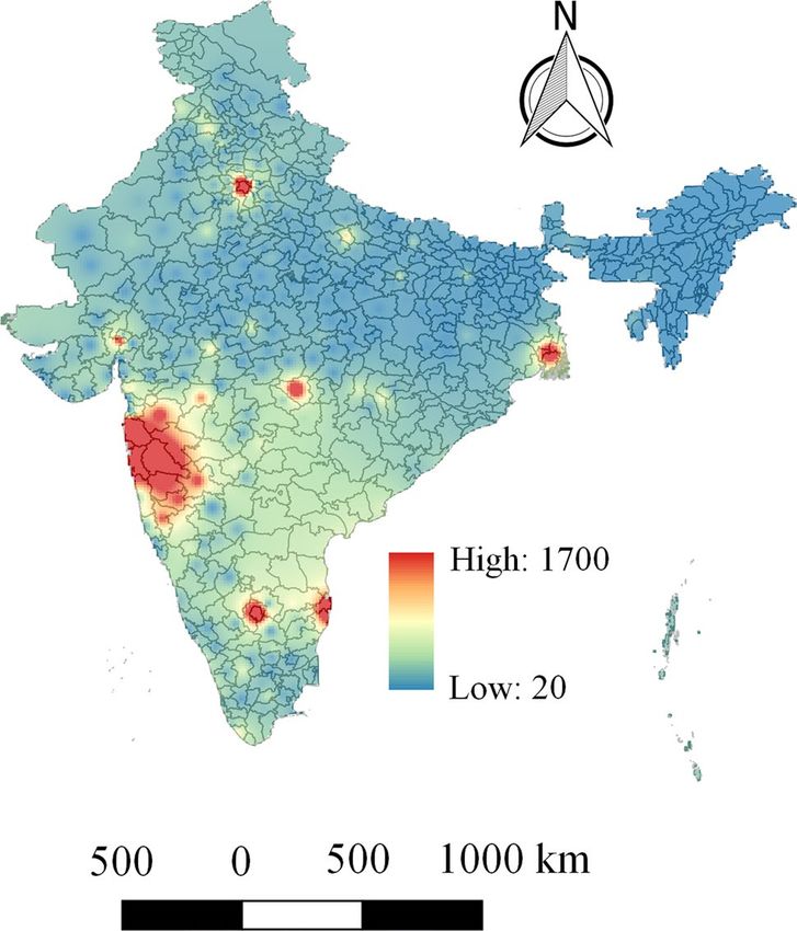
www.nature.com/scientificreports/
Dataset Dataset description Source Variable name Variable explanation
(i) COVID19INDIA website (https://
COVID-19 data from the states and www.covid19india.org/) (ii) Ministry
District-level COVID-19 death count
COVID-19 data union territories of India up to Febru- of Health and Family Welfare, Govern- COVID19_Death
up to February 24, 2021
ary 24, 2021. ment of India (https://www.mohfw.
gov.in/)
Tot_Population District-level total population
District-level count of total number of
HH_Above_8_P
households with at least 9 persons
District-level rate at which population
Growth_Rate
increases.
District-level count of the number of
Sex_Ratio
females per 1000 males
Contains district wise socioecono-mic India census, 2011 (https://censusindia. District-level count of total number of
Census data
and demographic data of India gov.in/) Age_Abv_50
persons with age 50 years or more
District-level count of total number of
HH_With_TCMC households having TV, Computer (or
laptop), Mobile phone, and Car.
District-level count of total number of
Higher_Edu
persons having higher education
District level percentage of urban
P_Urb_Pop
population
District-level exposure to PM2.5, aver-
aged across the period 2016 − 2020
PM2.5
January, 2016 to January, 2020) for a
Concentration of air pollutants (from (i) Central Pollution Control Board total of 130 monitoring stations
Environmental air pollution data January, 2016 to January, 2020) for a (CPCB), Government of India (https://
District-level exposure to NO2, aver-
total of 130 monitoring stations cpcb.nic.in/) NO2
aged across the period 2016 − 2020
District-level exposure to SO2, aver-
SO2
aged across the period 2016 − 2020
Table 1. A summary of datasets.
Additionally, the district-level data of each district needs to be linked with the GPS coordinate of the centroid
of that district. The dataset containing GPS coordinates of the districts of India are collected from Kaggle (https://
www.kaggle.com/sirpunch/indian-census-data-with-geospatial-indexing).
Data preparation. From the raw datasets, a total of eleven potential demographic, socioeconomic, and envi-
ronmental pollution related factors (see Table 1) are selected to explain the district-level geographical variation
of COVID-19 mortality. The district-level demographic and socioeconomic factors that are selected in this study
are: population; households with at least 9 persons; growth rate; sex ratio; persons with age 50 years or more;
households having TV, computer (or laptop), mobile phones and car; number of persons having higher educa-
tion; the percentage of the urban population. On the other hand, the environmental pollution related variables
that are selected are as follows: PM2.5 exposure; NO2 exposure; SO2 exposure.
The district-level long-term exposure to three air pollutants namely PM2.5, NO2, and SO2 are calculated from
the raw data of 130 pollution monitoring stations. The mean concentration of each of the above-mentioned
air pollutants of all the 130 monitoring stations is computed for the period 2016–2020. For each pollutant, the
computed values are spatially aggregated by averaging the values of all monitoring stations of a district. If a
district doesn’t contain any monitoring stations, then it’s exposure to that pollutant is computed using Nearest
Neighbour interpolation (NNI).
A multicollinearity verification is performed via the Variance Inflation Factor (VIF) to remove unnecessary
redundancy among the explanatory variables. VIF can be expressed as follows [Eq. (1)]:
1
VIF k = (1)
1 − Rk2
SSEk
Rk2 = 1 − (2)
SSTk
where, Rk2 denotes the coefficient of determination that is computed by regressing the kth variable on remain-
ing explanatory variables. The mathematical expression for Rk2 is given in Eq. (2). Here, SSEk and SSTk denote
the sum of squares of total variation and sum of squares of errors respectively. Firstly, regression analysis is
conducted among all the 11 explanatory variables to compute the VIFs that are shown in Table 2. It is observed
that the variable HH_Abv_8_P has high Variance Inflation Factor (VIF = 12.4). Now, if VIFs are larger than
10, it indicates that there is multicollinearity16. Eventually, the variable HH_Abv_8_P is removed from the set
of explanatory variables. After that, the regression is again performed on the remaining 10 variables, with the
Scientific Reports | (2021) 11:7890 | https://doi.org/10.1038/s41598-021-86987-5 3
Vol.:(0123456789)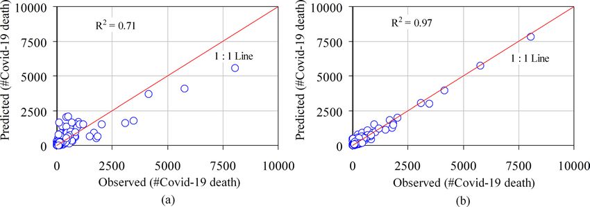
www.nature.com/scientificreports/
Variable VIF
Tot_Population 7.92
Growth_Rate 1.24
Sex_Ratio 1.30
HH_With_TCMC 3.91
HH_Abv_8_P 12.4
Higher_Edu 3.12
PM2.5 2.65
Age_Abv_50 3.47
P_Urb_Pop 1.93
SO2 1.20
NO2 1.52
Table 2. VIFs with all the 11 explanatory variables.
Variable VIF
Tot_Population 3.93
Growth_Rate 1.21
Sex_Ratio 1.32
HH_With_TCMC 2.96
Higher_Edu 2.94
PM2.5 2.35
Age_Abv_50 2.87
P_Urb_Pop 1.80
SO2 1.19
NO2 1.54
Table 3. VIFs after removing the variable HH_Abv_8_P.
VIFs given in Table 3. Now, it is observed that no VIF exceeds 10 eventually this set of 10 variables can be used
for model building.
Modeling spatial relationship. In this paper, the OLS (Ordinary Least Square) and GWR (Geographi-
cally Weighted Regression) models are utilized to determine the geographical relationship of COVID-19 mortal-
ity with potential risk factors.
The OLS method generally attempts to understand the global relationships between the dependent and
independent variables. In this case, the regression and its parameters are unchanged over the geographic space.
Mathematically, Eq. (3) represents a global regression model as follows:
n
Yi = η0 + ηk Xik + δi (3)
k=1
where, Yi denotes the dependent or response variable; Xik is the ith observation of kth independent variable;
ηk the global regression coefficient for kth independent variable; η0 represent the intercept parameter; and δ0
denotes the error term.
GWR technique extends the global regression [Eq. (3)] by enabling local parameter estimation13. It allows
regression coefficients to be a function of geographical location. In other words, the regression coefficients are
quantified independently in different geographical locations. A GWR model [Eq. (4)] can be represented as
follows:
n
Yi = ξi0 + ξk (µi , νi )Xki + δi (4)
k=1
where, Yi , Xki , and δi denote the dependent (or response) variable, kth independent (or predictor) variable, and
error at location i respectively; (µi , νi ) denotes coordinates of location i; ξk (µi , νi ) represent local coefficient for
kth predictor at location i. Note that, GWR model allows regression parameters to vary continuously across the
geographic space. For each location i, a set of regression parameters is estimated. The estimation of parameters
can be performed as follows:
Scientific Reports | (2021) 11:7890 | https://doi.org/10.1038/s41598-021-86987-5 4
Vol:.(1234567890)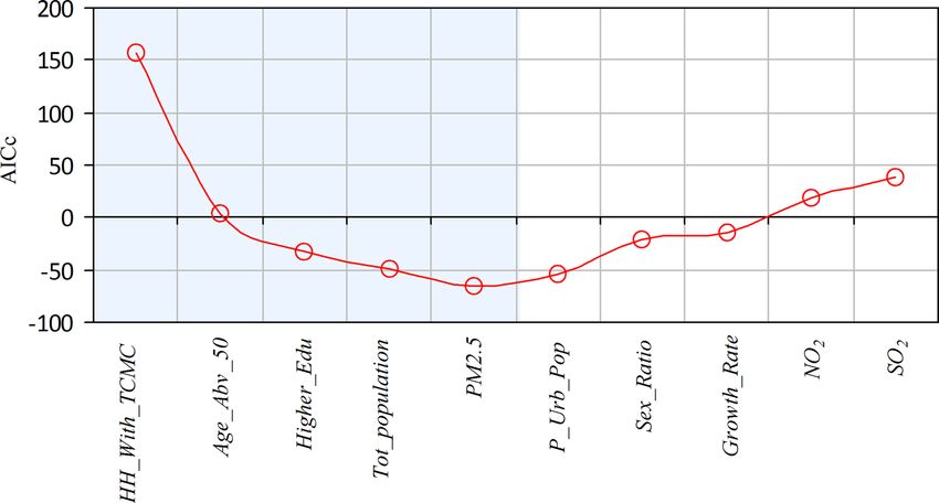
www.nature.com/scientificreports/
ξ (µ, ν) = (X T W(µ, ν)X )−1 X T W(µ, ν)Y
(5)
where, X denotes a matrix containing the values of independent variables and a column of all 1s; Y represents a
vector of values of the dependent variable;
ξ (µ, ν) is a vector of local regression parameters; W(µ, ν) is a diagonal
matrix whose diagonal elements represent the geographical weighting of the observations for regression location.
The weights in W(µ, ν) assigns greater weights to the observations that are closer to the regression point than
the observations that are farther away. In this work, the weights are computed using a Gaussian kernel function
which is defined as follows:
j
2
D j
wij = exp − 21 Bi , if Di ≤ B
(6)
wij = 0, otherwise
j
where, B represents the bandwidth and Di denotes the distance between the regression point i and the location
of observation j. Note that, the bandwidth can be defined either by a fixed number of closest neighbors (known
as adaptive bandwidth) or by a fixed distance (known as fixed bandwidth). Golden Section search17 is utilized
to find the optimum size of the bandwidth for GWR.
Performance metrics. The performance of the models are assessed by three metrics namely R2, adjusted R2,
and AICc. Here, AICc is a corrected version of the Akaike Information Criterion (AIC). AICc can be defined as
follows13:
N + tr(S)
AICc = N ln(2π) + 2N ln(σ̂ ) + N × (7)
N − 2 − tr(S)
where, N denotes the sample size, S is the hat matrix, tr(S) denotes the trace of S, and σ̂ represents the estimated
standard deviation of the error term. AICc denotes model’s accuracy and lower AICc indicates better model
quality. It is usually used to find the best-fit model. The value of R2 represents the ability of a model to explain
the variance in the dependent variable and therefore a larger R2 signifies the better performance of the model.
It is computed from the estimated and the actual values of the dependent variable. Moreover, Moran’s I index is
computed to investigate the spatial autocorrelation of the model residuals. Mathematically, it is defined as follows:
N
N N i=1 j=1 wij (yi − ȳ)(yj − ȳ)
I =
(8)
N N N 2
i=1 j=1 wij i=1 (yi − ȳ)
where, N denotes total number of observations, yi and yj are variable values at location i and j respectively, ȳ
represents the mean value, and wij denotes a weight between location i and j. The value of Moran’s I index can
vary between − 1 (perfect dispersion) to + 1 (a perfect positive autocorrelation). Note that, a zero value indicates
perfect spatial randomness.
Model building. Here, a step-wise GWR model selection using AICc is presented that can be utilized to inves-
tigate geographically varying relationships of COVID-19 mortality with different driving factors. The following
are the steps to build an appropriate GWR model18.
• Step 1 Suppose there are n explanatory variables (in our case n = 10). For each of the explanatory variables,
fit a separate GWR model by regressing that variable against the COVID19_Death variable. Compute AICc
for each of the n = 10 models. Find the model that generates the lowest AICc and permanently include the
corresponding explanatory variable in subsequent model building.
• Step 2 Subsequently select a variable from the remaining (n − 1) variables, build a model with the perma-
nently included variables along with the newly selected variable. Find the explanatory variable that produces
the lowest AICc and permanently include it in subsequent model building. Set n = n − 1.
• Step 3 Repeat Step 2 until it is observed that there is no reduction in AICc.
The above-mentioned steps are carried out using MGWR 2.2 software19. When calibrating the GWR, an adaptive
bisquare spatial kernel is applied. Moreover, in order to select an optimal bandwidth, the Golden Section s earch17
is employed. Figure 2 shows the changes in AICc during the step-by-step selection of explanatory variables for
model building. It is observed that after the inclusion of a total of five variables, the AICc values start increasing
when further new variables are included. Note that, both a global (OLS) model and a local (GWR) model are
calibrated with these five explanatory variables.
Results
In this section, firstly the performance of the global model (OLS) and local model (GWR) are discussed. Next,
the geographically varying relationships of COVID-19 mortality with different factors are presented.
Performance of OLS and GWR model. A detailed summary of the OLS model is presented in Table 4.
The variables Tot_population, HH_With_TCMC, Age_ABV_50, and PM2.5 returns significant t values of 2.91,
12.114, − 1.225 and − 2.485 respectively. Moreover, the Moran’s I of the residuals of the global OLS model are
also analysed. It is found that there is significant spatial autocorrelation (Moran’s I = 0.348 and p < 0.01). The
Scientific Reports | (2021) 11:7890 | https://doi.org/10.1038/s41598-021-86987-5 5
Vol.:(0123456789)www.nature.com/scientificreports/
Figure 2. Stepwise variable selection for geographically weighted regression (GWR).
Variable Coef. Est Est Err t statistic p-value
Intercept 0.000 0.026 0.000 1.000
Tot_population 0.322 0.11 2.91 0.005*
HH_With_TCMC 0.675 0.045 12.114 0.000*
Age_Abv_50 0.125 0.102 – 1.225 0.050*
Higher_Edu 0.136 0.073 1.851 0.064
PM2.5 – 0.079 0.032 – 2.485 0.013*
Table 4. Summary of the global model (OLS) for various socioeconomic, demographic, and environmental
pollution related factors. *Significant at 0.05.
Variable Mean STD Min Median Max
Intercept 0.413 0.292 – 0.789 0.043 1.134
Tot_population 0.152 0.604 – 2.525 0.126 1.385
HH_With_TCMC 0.520 0.382 – 0.258 0.408 2.550
Age_Abv_50 0.317 0.648 – 1.016 0.189 2.861
Higher_Edu – 0.038 0.381 – 1.566 – 0.025 1.488
PM2.5 0.101 0.352 – 1.721 0.015 0.842
Table 5. Summary of the local model (GWR) for various socioeconomic, demographic, and environmental
pollution related factors.
assumptions of OLS estimation are violated as there exist dependent residuals. Eventually, the GWR model is
utilized to show the geographical variations of the relationships with different factors. A detailed summary of the
GWR model for the local parameter estimates is presented in Table 5.
The performance of OLS and GWR model in terms of R2 , Adj R2 , and AICc are also provided in Table 6.
Moreover, Fig. 3a and b show the scatter plots between predicted and observed COVID-19 death count using
the global OLS and GWR models. These figures indicate that the GWR model resulted in a better fit as compared
to the global OLS model. This is because, in the case of GWR, the predicted values are closely distributed along
the 1:1 line relative to the observed values. The global model explains only 71.9% of the variance of district-level
COVID-19 deaths which is increased to 97% if the model is calibrated as GWR by taking into account the local
impact of the explanatory variables. Comparing the models in terms of AICc, show that the model fit is greatly
enhanced by reducing the value of AICc from 655.835 (OLS model) to -66.42 (GWR model). Moreover, the
verification of Moran’s I of the residuals of the GWR model indicates that the residuals are randomly distributed
(Moran’s I=-0.0395 and p < 0.01). In other words, the residuals don’t have any significant spatial autocorrelation
and eventually, it shows the suitability of GWR over the global model (OLS).
Scientific Reports | (2021) 11:7890 | https://doi.org/10.1038/s41598-021-86987-5 6
Vol:.(1234567890)www.nature.com/scientificreports/
Performance metrics OLS GWR
AICc 655.835 – 66.42
R2 0.719 0.97
Adj R2 0.715 0.964
Table 6. Performance comparison OLS and GWR models in terms of three performance metrics: AICc, R2,
and Adjusted R2.
Figure 3. Scatter plot of the observed and the predicted COVID-19 death count using (a) global OLS model
and (b) GWR model.
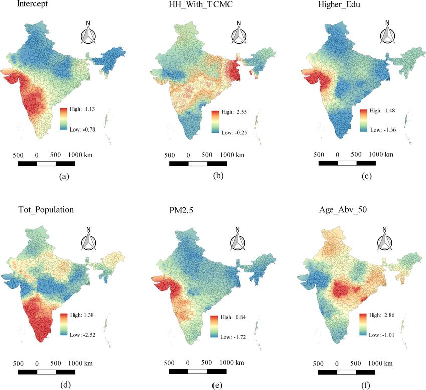
Figure 4. Geographical distribution of R2 values for geographically weighted regression (GWR) model.
Geographically varying relationships between COVID‑19 deaths and the driving factors. The
geographical distribution of R2 is presented in Fig. 4 that shows it varies within a range 0.42–0.97. It is found that
more than 86% of local R2 values are larger than 0.60 and almost 68% of R2 values are within the range 0.80–0.97.
Note that, very high R2 values are mainly observed in the western and the eastern regions of India. Moreover, low
and moderate R2 values are mainly distributed over the northern and the southern part of India.
Scientific Reports | (2021) 11:7890 | https://doi.org/10.1038/s41598-021-86987-5 7
Vol.:(0123456789)www.nature.com/scientificreports/
Figure 5. Local parameter estimates of geographically weighted regression (a) Intercept (b) HH_With_TCMC
(c) Higher_Edu (d) Tot_population (e) PM2.5 and (f) Age_Abv_50.
Now, the geographical distribution of local coefficient estimates of the GWR model is provided in Fig. 5
to further reveal the relationship of the explanatory variables with the COVID-19 deaths. It mainly facilitates
understanding of the complex relationship that varies over the geographic space. The results of GWR in Fig. 5
not only present positive or negative relationships but also show whether the relationship is strong or weak. A
positive relationship indicates that the COVID-19 deaths tend to increase as the value of specific explanatory
variable increases. A negative relationship indicates that the COVID-19 deaths tend to decrease as the value of
specific explanatory variable increases. Moreover, larger values of a coefficient denote a stronger relationship. In
the maps of Fig. 5, the regions having deep red shade denote regions in which the specific variable has a strong
positive influence (i.e. strong positive relationship) on COVID-19 deaths.
As shown in Fig. 5a, the GWR model produces local intercept that can vary within the range – 0.78 to 1.13
with a mean of 0.013. In Fig. 5b, the regions with deep red color (mainly the state of West Bengal) denote those
areas where the variable HH_With_TCMC has a strong positive relationship with COVID-19 death. The variable
Higher_Edu is a strong predictor (See Fig. 5c) for COVID-19 death in some parts of western India (mainly the
state of Gujarat), southern India (mainly the states of Tamil Nadu and Kerala), and Eastern India (mainly the
state of West Bengal). On the other hand, in the southern and the south-western part of India, a positive relation-
ship between population and COVID-19 death is found (see Fig. 5d). However, in some regions of central and
western India (the states of Madhya Pradesh and Gujarat), a strong negative relationship between population
and COVID-19 death is also observed. Fig. 5e shows that mainly in the western part of India there is a strong
positive relationship between PM2.5 and COVID-19 death, whereas in the other parts of India there is no such
Scientific Reports | (2021) 11:7890 | https://doi.org/10.1038/s41598-021-86987-5 8
Vol:.(1234567890)www.nature.com/scientificreports/
Parameter estimates
District Local R2 Intercept PM2.5 Tot_population HH_With_TCMC Age_Abv_50 Higher_Edu
Pune 0.982 0.219 − 0.221 − 0.311 0.661 − 0.154 0.768
Mumbai 0.981 0.654 0.712 − 0.388 0.859 − 0.074 0.719
Thane 0.986 0.086 0.806 − 0.958 0.716 − 0.084 0.897
Chennai 0.978 0.234 0.421 0.689 1.089 − 0.496 − 0.575
Kolkata 0.987 0.057 − 0.055 − 0.146 1.114 0.658 − 0.152
Nashik 0.986 0.030 0.800 − 0.280 0.742 0.079 0.985
Jalgaon 0.966 0.099 0.357 − 0.389 0.744 0.284 0.853
Nagpur 0.955 0.088 − 0.132 − 1.214 0.685 1.588 − 0.571
Solapur 0.974 0.318 0.476 0.516 0.685 − 0.073 0.241
Kolhapur 0.972 0.238 0.249 0.483 0.791 − 0.142 0.244
Surat 0.976 0.223 0.749 − 1.189 0.481 − 0.127 1.469
Sangli 0.973 0.281 0.399 0.358 0.576 − 0.324 0.127
Ludhiana 0.921 − 0.037 − 0.175 − 0.189 0.287 0.423 − 0.225
Chittoor 0.973 − 0.029 0.102 0.562 0.128 0.117 − 0.286
East Godavari 0.959 0.159 − 0.159 − 0.541 1.078 0.458 − 0.654
Indore 0.798 0.011 0.062 0.141 − 0.180 − 0.120 0.323
Guntur 0.954 0.150 0.116 0.274 − 0.185 0.247 − 0.142
Lucknow 0.984 − 0.043 − 0.104 0.049 0.389 − 0.109 0.284
Satara 0.978 0.264 0.370 0.196 0.793 − 0.222 0.482
Kurnool 0.856 0.229 0.392 0.366 0.371 0.144 0.096
Madurai 0.950 0.143 0.078 0.629 0.162 − 0.059 − 0.651
Anantapur 0.886 0.094 0.167 0.226 0.107 0.258 − 0.125
Dharwad 0.948 0.193 0.283 0.523 0.741 − 0.139 0.105
West Godavari 0.954 0.166 − 0.068 0.029 0.322 0.198 − 0.284
Coimbatore 0.934 − 0.145 0.099 0.578 0.321 − 0.127 − 0.381
Prakasam 0.953 0.137 0.071 0.324 − 0.179 0.314 − 0.101
Bhopal 0.916 − 0.044 0.037 − 0.296 0.475 0.295 0.125
Krishna 0.937 0.151 − 0.074 0.221 0.102 0.194 − 0.214
Latur 0.967 0.348 0.356 0.571 0.598 0.542 − 0.293
Jaipur 0.797 − 0.143 − 0.131 0.019 0.289 0.225 − 0.126
Srikakulam 0.920 0.086 0.108 − 1.146 0.854 1.285 − 0.276
Nanded 0.960 0.255 0.117 − 0.076 0.725 1.108 − 0.508
Dhule 0.966 0.074 0.533 − 0.746 0.385 − 0.278 1.175
Hassan 0.683 0.065 0.214 0.417 0.401 0.112 − 0.419
Table 7. Local R2 and district-level parameter estimates by geographically weighted regression for some of the
districts of India that are severely affected by COVID-19 disease.
strong relationship. The explanatory variable Age_Abv_50 shows a positive relationship in central, eastern, and
northern parts of India (see Fig. 5f).
Moreover, Table 7 represents the district-level results of the local model (GWR) for some of the districts that
are severely affected by COVID-19 disease. The local R2 values revealed district-level variability in GWR model
performance. Specifically, the local R2 values could be helpful here to see where geographically weighted regres-
sion predicts well and where it predicts poorly. It is observed that the GWR model yields high local R2 value for
most of the heavily affected districts. For instance, very high local R2 values are found for the following districts:
Pune ( R2 = 0.982 ), Thane ( R2 = 0.986 ), Lucknow ( R2 = 0.984 ), Chittor ( R2 = 0.973), Nasik ( R2 = 0.986 ),
Solapur ( R2 = 0.974 ), Kolhapur ( R2 = 0.972), Sangli ( R2 = 0.973), Satara ( R2 = 0.978), Latur ( R2 = 0.967 ),
Mumbai (R2 = 0.981), Kolkata (R2 = 0.987), Chennai (R2 = 0.978), Jalgaon (R2 = 0.966), Nanded (R2 = 0.960).
On the other hand, moderate local R2 values are found for Dharwad (R2 = 0.948), Nagpur (R2 = 0.955), Srikaku-
lam (R2 = 0.920), Ludhiana (R2 = 0.921), Guntur (R2 = 0.95), Kurnool (R2 = 0.856), Coimbatore (R2 = 0.934),
West Godavari ( R2 = 0.95), Anantapur ( R2 = 0.886 ), Bhopal ( R2 = 0.916 ), and Krishna ( R2 = 0.937 ). The
lowest R2 values are observed for the following districts: Hassan ( R2 = 0.683), Indore ( R2 = 0.798 ), and
Jaipur ( R2 = 0.797 ). Note that, for most of the highly COVID-19-affected districts, the variables PM2.5 and
HH_With_TCMC are usually exhibited positive relationships in regression modeling. On the other hand, the
variable Higher_Edu usually exhibits negative relationships for most of the highly affected districts.
Scientific Reports | (2021) 11:7890 | https://doi.org/10.1038/s41598-021-86987-5 9
Vol.:(0123456789)www.nature.com/scientificreports/
Discussion
In order to better understand how different driving factors influence the overall fatalities caused by COVID-19,
the geographical distribution of COVID-19-related deaths are investigated. The highest number of COVID-19-re-
lated deaths are found primarily in the western part of India (Pune, Thane, Mumbai, Nagpur, Nashik, Raigad,
Jalgaon, Kolhapur, Sangli, Satara, Solapur, Ahmedabad, Surat). On the other hand, the number of COVID-
19-related deaths is relatively low in the northern and eastern parts of India. This study identified considerable
geographical variability of COVID-19 deaths and their heterogeneous relationship at the local level with the
driving factors in India. More specifically, the utilization of the GWR method successfully found the geographi-
cally varying relationship of COVID-19 mortality with various potential socio-economic, demographic, and envi-
ronmental pollution related factors. This study reveals five important local factors are significantly related with
district-level COVID-19 deaths as follows: (i) population (ii) PM2.5 level (iii) households having TV, computer
(or laptop), mobile phones and car (iv) persons with age 50 years or more (v) number of persons having higher
education. Furthermore, this study also validates the effectiveness of local parameter estimation by comparing
the global OLS method with the local GDR method. To the best of our knowledge, this is the first study that
explores geographically varying relationships of COVID-19 deaths with various potential driving factors in India.
Rigorous analyses are performed to demonstrate the shortcomings of global technique (OLS) as compared
to the local technique (GWR) in terms of several performance metrics. The OLS model only explains 71.9% of
the variance of district-level COVID-19 deaths. It is found that the predictive efficiency and model accuracy
are further enhanced by implementing the GWR method. The GWR model explains 97% of the variance of
district-level COVID-19 deaths. Moreover, Moran’s I index verifies that no significant spatial autocorrelation is
present in the residuals of the GWR model. Note that, a key advantage of such a local method is its capability to
visualize the geographically varying heterogeneous relationships between the dependent and the independent
variables. In other words, it enables us for a better understanding of relationships based on geographical contexts
and study area’s known features.
The findings of this study reveal that there are strong positive relationships of COVID-19 deaths with the
explanatory variables PM2.5 and Tot_population across the regions of the COVID-19 death hotspots in the west-
ern part of India. The positive association of COVID-19 deaths with long term exposure of PM2.5 is consistent
with the previous works20,21. Note that, long-term PM2.5 exposure is substantially associated with some of the
comorbidities (e.g. chronic lung disease, cardiovascular disease, etc.) that may lead to COVID-19 deaths22,23.
Similarly, a positive association between COVID-19-related deaths and Tot_population is also observed in other
studies6,24. However, the reverse association is found for these two variables ( PM2.5 and Tot_population) in the
other parts of India. The explanatory variable HH_With_TCMC is found to be an important factor that may
be a measure of the number of households with the upper class and rich people. A strong positive relationship
is observed between HH_With_TCMC and COVID-19 death in the hotspots of eastern and western parts of
India (Kolkata, North 24 Parganas, Pune, Thane, Surat, Nagpur, etc.). Note that, in those hotspots, the value
of HH_With_TCMC is substantially high. An interesting observation reveals that a strong negative relation-
ship exists between COVID-19 death and Higher_Edu in the eastern, central, and southern parts of India. It is
expected that the higher educated people are well aware of the symptoms and the complications of COVID-19
that may lead to the fewer number of fatalities in those regions. Now, in some regions of the south-eastern part
of India, the number of COVID-19 deaths is also seen to be high.
In those regions, significant positive relationships are found between COVID − 19 deaths and Tot_population,
whereas significant negative relationships are observed for the variable Higher_Edu.
This research work inherits certain shortcomings that need to be resolved in future research. For instance,
there may have high possibilities of under-reporting in COVID-19 death counts that may introduce bias in the
study25. Moreover, due to data unavailability, we were not able to include some significant district-level driving
factors in our study, such as health care system quality, number of hospital beds, household income, and poverty
data. Despite the above-mentioned shortcomings, this is the first study that explores geographically varying
relationships of COVID-19 mortality with different socioeconomic, demographic, and environmental pollu-
tion related factors in India. This research work also highlights the significance of the geographically weighted
regression in the geographical analysis of the health outcome of COVID-19 disease.
Conclusion
COVID-19 pandemic is one of the most serious global public health catastrophe of the century. In this work,
the geographically varying relationships between COVID-19 deaths and different potential driving factors are
assessed across India. The geographical distribution of reported COVID-19 death cases is found to be heterogene-
ous over India. This heterogeneity in distribution is related to many underlying factors, including demographic,
socioeconomic, and environmental pollution related variations between different parts of India. The GWR model
makes it possible for the regression coefficients to differ across the geospace, creating geographical patterns about
the strength of the relationship. The geographical heterogeneity and non-stationary of the relationships between
COVID-19 deaths and the driving factors are demonstrated by mapping the local parameter estimates. The local
parameter estimates reflect the quality of local model fitting and the nature of the association. The local method
(GWR) yields better performance with smaller AICc as compared to the global method (OLS).
It should be noted that the impacts of other influencing factors (e.g. Meteorological factors) are not included
in this work. This might be the direction for future studies. Moreover, in this study, currently we do not consider
time evolution of variables, it is because for the dependent and the independent variables we may require more
time series data for the effective temporal modelling. However, we plan to consider the time evolution of the
variables for the future studies when more time series data will be available.
Scientific Reports | (2021) 11:7890 | https://doi.org/10.1038/s41598-021-86987-5 10
Vol:.(1234567890)www.nature.com/scientificreports/
Received: 19 October 2020; Accepted: 22 March 2021
References
1. WHO Coronavirus Disease (COVID-19) Dashboard. (2020). https://covid19.who.int/.
2. Zhou, F. et al. Clinical course and risk factors for mortality of adult inpatients with covid-19 in Wuhan,China: A retrospective
cohort study. Lancet (2020).
3. Garg, S. Hospitalization rates and characteristics of patients hospitalized with laboratory-confirmed coronavirus disease
2019-covid-net, 14 states, March 1–30, 2020. Morb. Mortal. Wkly. Rep. 69, (2020).
4. Li, K. et al. The clinical and chest ct features associated with severe and critical covid-19 pneumonia. Investig. Radiol. (2020).
5. Ehlert, A. The socioeconomic determinants of covid-19: A spatial analysis of german county level data. medRxiv (2020).
6. Sannigrahi, S., Pilla, F., Basu, B., Basu, A. S. & Molter, A. Examining the association between socio-demographic composition and
covid-19 fatalities in the european region using spatial regression approach. Sustain. Cities Soc. 62, 102418 (2020).
7. Gupta, A., Banerjee, S. & Das, S. Significance of geographical factors to the covid-19 outbreak in india. Model. Earth Syst. Environ.
1–9, (2020).
8. Sun, F., Matthews, S. A., Yang, T.-C. & Hu, M.-H. A spatial analysis of the covid-19 period prevalence in us counties through june
28, 2020: Where geography matters?. Ann. Epidemiol. (2020).
9. Hutcheson, G. D. Ordinary Least-Squares Regression 224–228 (L. Moutinho and GD Hutcheson, The SAGE dictionary of quantita-
tive management research, 2011).
10. Brunsdon, C., Fotheringham, S. & Charlton, M. Geographically weighted regression: A method for exploring spatial nonstationar-
ity. Encycl. Geogr. Inf. Sci. 558, (2008).
11. Cressie, N. Statistics for Spatial Data ( Wiley, 2015).
12. Wheeler, D. C. & Páez, A. Geographically weighted regression. In Handbook of Applied Spatial Analysis, 461–486 (Springer, 2010).
13. Fotheringham, A. S., Brunsdon, C. & Charlton, M. Geographically Weighted Regression: The Analysis of Spatially Varying Relation-
ships (Wiley, 2003).
14. Anselin, L. Local indicators of spatial association-lisa. Geogr. Anal. 27, 93–115 (1995).
15. Central Pollution Control Board, Ministry of Environment, Forest and Climate Change, Govt. of India. (2020). https://cpcb.nic.
in/.
16. Menard, S. Applied logistic regression analysis. Sage 106, (2002).
17. Golden, B. L. & Wasil, E. A. Optimisation [by dm greig (london: Longman, 1980, 179 pp.)]. IEEE Trans. Syst. Man Cybern. 12, 684
(1982).
18. Yang, W. An Extension of Geographically Weighted Regression with Flexible Bandwidths. Ph.D. thesis, University of St Andrews
(2014).
19. Oshan, T. M., Li, Z., Kang, W., Wolf, L. J. & Fotheringham, A. S. mgwr: A python implementation of multiscale geographically
weighted regression for investigating process spatial heterogeneity and scale. ISPRS Int. J. Geo-Inf. 8, 269 (2019).
20. Wu, X., Nethery, R. C., Sabath, B. M., Braun, D. & Dominici, F. Exposure to air pollution and covid-19 mortality in the United
States. medRxiv (2020).
21. Magazzino, C., Mele, M. & Schneider, N. The relationship between air pollution and covid-19-related deaths: An application to
three french cities. Appl. Energy 115835, (2020).
22. Brook, R. D. et al. Particulate matter air pollution and cardiovascular disease: An update to the scientific statement from the
american heart association. Circulation 121, 2331–2378 (2010).
23. Sanyaolu, A. et al. Comorbidity and its impact on patients with covid-19. SN Compreh. Clin. Med. 1–8, (2020).
24. Su, D. et al. Influence of socio-ecological factors on covid-19 risk: a cross-sectional study based on 178 countries/regions worldwide.
Regions Worldwide (4/17/2020) (2020).
25. Chatterjee, P. Is India missing covid-19 deaths?. Lancet 396, 657 (2020).
Acknowledgements
This research work is supported by the project entitled- Participatory and Realtime Pollution Monitoring System
For Smart City, funded by Higher Education, Science & Technology and Biotechnology, Department of Science
& Technology, Government of West Bengal, India.
Author contributions
S.R. proposed the research topic, provided conceptual and technical guidance. A.I.M. designed the research
plan, wrote the manuscript, collected the data, performed the statistical analysis. A.I.M. and S.R. both involved
in the revision of the manuscript and interpretation of the results. Both the authors read and approved the final
manuscript.
Competing interests
The authors declare no competing interests.
Additional information
Correspondence and requests for materials should be addressed to S.R.
Reprints and permissions information is available at www.nature.com/reprints.
Publisher’s note Springer Nature remains neutral with regard to jurisdictional claims in published maps and
institutional affiliations.
Scientific Reports | (2021) 11:7890 | https://doi.org/10.1038/s41598-021-86987-5 11
Vol.:(0123456789)www.nature.com/scientificreports/
Open Access This article is licensed under a Creative Commons Attribution 4.0 International
License, which permits use, sharing, adaptation, distribution and reproduction in any medium or
format, as long as you give appropriate credit to the original author(s) and the source, provide a link to the
Creative Commons licence, and indicate if changes were made. The images or other third party material in this
article are included in the article’s Creative Commons licence, unless indicated otherwise in a credit line to the
material. If material is not included in the article’s Creative Commons licence and your intended use is not
permitted by statutory regulation or exceeds the permitted use, you will need to obtain permission directly from
the copyright holder. To view a copy of this licence, visit http://creativecommons.org/licenses/by/4.0/.
© The Author(s) 2021
Scientific Reports | (2021) 11:7890 | https://doi.org/10.1038/s41598-021-86987-5 12
Vol:.(1234567890)You can also read