Domain Adaptation without Source Data - arXiv
←
→
Page content transcription
If your browser does not render page correctly, please read the page content below
Domain Adaptation without Source Data

                                                 Youngeun Kim                        Donghyeon Cho                       Kyeongtak Han
                                                  Yale University               Chungnam National University              Inha University
                                             youngeun.kim@yale.edu                 cdh12242@gmail.com                  han00127@inha.edu

                                                                 Priyadarshini Panda                  Sungeun Hong
arXiv:2007.01524v4 [cs.CV] 30 Aug 2021

                                                                    Yale University                   Inha University
                                                               priya.panda@yale.edu                csehong@inha.ac.kr

                                                                                        Abstract

                                                  Domain adaptation assumes that samples from source and target domains are freely
                                                  accessible during a training phase. However, such an assumption is rarely plausible
                                                  in the real-world and possibly causes data-privacy issues, especially when the label
                                                  of the source domain can be a sensitive attribute as an identifier. To avoid accessing
                                                  source data that may contain sensitive information, we introduce Source data-Free
                                                  Domain Adaptation (SFDA). Our key idea is to leverage a pre-trained model from
                                                  the source domain and progressively update the target model in a self-learning
                                                  manner. We observe that target samples with lower self-entropy measured by the
                                                  pre-trained source model are more likely to be classified correctly. From this, we
                                                  select the reliable samples with the self-entropy criterion and define these as class
                                                  prototypes. We then assign pseudo labels for every target sample based on the simi-
                                                  larity score with class prototypes. Furthermore, to reduce the uncertainty from the
                                                  pseudo labeling process, we propose set-to-set distance-based filtering which does
                                                  not require any tunable hyperparameters. Finally, we train the target model with
                                                  the filtered pseudo labels with regularization from the pre-trained source model.
                                                  Surprisingly, without direct usage of labeled source samples, our SFDA outper-
                                                  forms conventional domain adaptation methods on benchmark datasets. Our code
                                                  is publicly available at https://github.com/youngryan1993/SFDA-SourceFreeDA.

                                         1   Introduction

                                         Supervised learning has proven outstanding performance in computer vision [1, 2, 3, 4, 5, 6, 7,
                                         8], however, performance degradation because of the differences observed from training and test
                                         environments is still problematic. The natural solution for reducing this environmental discrepancy is
                                         to collect a set of labeled samples from test-like environments and use them for training. Unfortunately,
                                         such rich supervision is not only time-consuming but also expensive due to the labeling costs in real
                                         world. In such situations, unsupervised domain adaptation [9], which can transfer knowledge from a
                                         labeled source domain to an unlabeled target domain during training, is an attractive alternative. For
                                         this reason, considerable effort has been devoted to unsupervised domain adaptation and has shown
                                         promising results in a variety of tasks [9, 10, 11, 12, 13, 14].
                                         In general, unsupervised domain adaptation assumes that data distribution from labeled source data
                                         and unlabeled target data are related but different [15], and all samples from both domains are freely
                                         available during the training process. However, this assumption is rarely possible in real-world and
                                         potentially can cause problems in terms of data privacy [16]. Suppose that the label of source data
                                         contains bio-metric information, e.g., face, fingerprint, iris pattern, or confidential information about
                                         specific individuals [17, 18, 19, 20]. From the security viewpoint, this kind of sensitive label can serve
                                         as an identifier for each sample or individual; thus, improper disclosure of data with corresponding

                                         Preprint. Under review.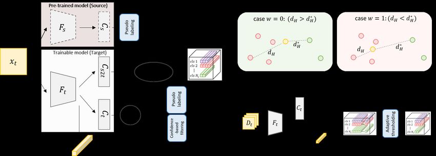
(a)                                           (b)
Figure 1: Normalized self-entropy statistics of target samples that passed through the pre-trained
source model (ResNet-50) on Ar ⇒ Cl in Office-Home. (a) The smaller the self-entropy value, the
higher the accuracy. Here, we define samples with higher accuracy than the average accuracy of the
total samples as “reliable samples” (shaded bins). (b) Unfortunately, these reliable samples account
for a small portion of the total samples. An in-depth analysis of the statistics regarding reliable
samples will be covered in Section 3.3.

labels could adversely affect data providers and related organizations. Indeed, privacy concerns have
increased considerably in recent years due to the possibility of leakage of sensitive data and the
vulnerability of centralized modeling. [21, 22].
In this paper, we propose a novel approach that can decouple the domain adaptation process from the
direct usage of source data by leveraging pre-trained source model, called Source data-Free Domain
Adaptation (SFDA). Our key idea is to update the target model using a pre-trained source model and
reliable target samples in a self-learning manner. The natural question that arises is how to select
reliable target samples from the pre-trained source model. In domain adaptation, source and the target
domains are closely related underPcovariate shift [15]. Also, prediction uncertainty can be quantified
by self-entropy, i.e., H(x) = − p(x)log(p(x)), where smaller entropy indicates more confident
prediction. Based on this, we hypothesize that among the unlabeled target samples, samples with low
self-entropy measured by the pre-trained source model are sufficiently reliable. To verify this, we
measure the self-entropy of target samples fed into a pre-trained source model and then analyze the
accuracy as well as the sample distribution. As shown in Fig. 1, we treat samples with the entropy
values less than 0.2 as “reliable samples", which accounts for about 30% of total samples. From the
results, we can conclude that a target model can be trained with reliable target samples through the
self-entropy criteria, but fatally, there are very few such samples.
To address the issue of reliable, yet, very few target samples, we propose a new framework consisting
of two parts. One is a pre-trained model from the source domain where all the weights are frozen,
and the other is a target model that is initialized from the pre-trained source model but evolves
progressively by optimizing two losses (see Fig. 2). The first loss uses source-oriented pseudo labels
of all target samples from the pre-trained source model; this prevents the target model from a self-
biasing problem caused by the second self-learning loss. The second loss optimizes the target model
using the target-oriented pseudo labels of target samples obtained from the trainable target network.
More precisely, we periodically store low-entropy reliable samples for each class as prototypes in a
memory bank during the training process. Then, we assign target-oriented pseudo labels to a target
sample based on the similarity between embedded features and stored class prototypes. However,
pseudo labels may not be always accurate. So, we propose a confidence-based sample filtering by
measuring set-to-set distance. As training goes on, we gradually increase the impact of the second
loss, allowing our target model to adapt to the target domain in a progressive manner.
The main contributions of this work can be summarized as follows. (i) We tackle domain adaptation
under environments with data-privacy issues. To the best of our knowledge, this is the first work
on domain adaptation without any source data in training. (ii) To decouple domain adaptation from
source data, we propose a novel framework that progressively evolves based on only reliable target
samples with regularization from the source domain information. (iii) Although we train our target
model without any source samples, our method achieves higher performance than conventional
models trained with labeled source data.

                                                  2
Figure 2: Overall flow of SFDA framework. Dashed lines indicate fixed model parameters.
2 Source data-free domain adaptation
2.1 Problem setup
The main distinction between unsupervised domain adaptation (UDA) and our proposed SFDA is
that we do not use any labeled source samples during the training process. To clarify this, we first
describe the configuration of unsupervised domain adaptation and then introduce the setting of the
proposed SFDA.
Unsupervised domain adaptation: The main goal of UDA is to minimize discrepancy between a
labeled source domain Ds = { xis , ysi }N s
i=1 and an unlabeled target domain Dt = {xjt }N t
j=1 , where
Ns and Nt denote the number of source and target samples, respectively. The main assumption of this
task is that source and target samples are drawn from a different but related probability distribution
Ds ∼ ps and Dt ∼ pt , according to covariate shift [15].
Unsupervised domain adaptation without source data: Unlike UDA, the proposed SFDA protocol
assumes that we cannot access samples from a source domain due to privacy issues. Instead of using a
source dataset, this new protocol exploits a pre-trained model from the source domain. More precisely,
SFDA aims to perform unsupervised domain adaptation through the parameters of a pre-trained
source model θs and the unlabeled target domain Dt = {xjt }N t
j=1 .
2.2 SFDA framework
Figure 2 illustrates the overall flow of the proposed method. Our SFDA framework contains two
types of models: a pre-trained source model and a trainable target model. The source model consists
of a feature extractor Fs and a classifier Cs , and all parameters of these modules are fixed after being
pre-trained from the source domain. The trainable target model consists of a feature extractor Ft
with multi-branch classifiers, Cs2t and Ct , and the parameters of each module are initialized by the
parameter of pre-trained source model, i.e., θFs and θCs . When target samples are given as input to
Ft , the upper branch, i.e., Cs2t , is trained with the source-oriented pseudo labels yˆs obtained from the
pre-trained classifier Cs . On the other hand, the lower branch, i.e., Ct , is trained using target-oriented
pseudo labels yˆt obtained by the proposed adaptive prototype memory. Once the pseudo labels yˆt are
obtained through adaptive prototype memory, we additionally remove unreliable samples through
set-to-set distance-based confidence. Overall, we adapt the target model to the target domain using
pseudo labels yˆt in a self-learning manner, while using source knowledge yˆs from the pre-trained
source model as a regularizer.
Adaptive prototype memory: Our target model updates model parameters from two types of loss
functions. The first loss function in Cs2t aims to maintain the information of the source domain. For
this, Cs2t uses the pseudo labels obtained after inferring the target samples through the pre-trained
source model, i.e., Fs and Cs . Crucially, all the parameters of the pre-trained model are fixed. Hence,
the loss of Cs2t for each target sample does not change during the training process.
To evolve the target model during training, we assign pseudo labels for all target samples by us-
ing Adaptive Prototype Memory (APM). The proposed APM consists of reliable target samples
for each class called multi-prototypes. As a first step, we compute the normalized self-entropy
31
P
H(xt ) = − logN c
l(xt )log(l(xt )) of target samples where l(xt ) denotes the predicted probability
by classifier Ct , and Nc refers to the total number of classes. We then construct a class-wise entropy
set Hc = {H(xt )|xt ∈ Xc }, where Xc denotes the set of samples predicted by Ct as class c.
The next step is to choose reliable samples, called multi-prototypes, which can represent each class.
One naïve approach for this is to select a fixed number of samples with low self-entropy per class.
However, each class might have different entropy distribution resulting in certain classes having
lower average self-entropy than others. To address this issue, we propose an approach that can
adaptively have a different number of prototypes for each class. We first find the lowest entropy
for each class, then set the largest value among them as the threshold for selecting prototypes,
i.e., η = max {min(Hc )|c ∈ C}, where C = {1, ..., Nc } is a class set. The main advantage of this
technique is that a threshold for reliable sample selection can be obtained adaptively in the training
process without any hyper-parameters. Using this adaptive threshold, we obtain multiple prototypes
for each class as follows:
Mc = {Ft (xt )|xt ∈ Xc , H(xt ) ≤ η} . (1)
Note that each prototype consists of an embedded feature Ft (xt ). Since multiple prototypes are later
used for pseudo-labeling and confidence-based filtering, we store all prototypes into APM. Updating
APM at every training step incurs a high computational cost, so we update APM periodically.
Empirically, we update APM every 100 steps across all datasets. The entire procedure of APM is
described in Algorithm 1.
Pseudo labeling: Based on the multi-prototypes in APM, we can assign pseudo labels to unlabeled
target samples. Given a target sample xt ∈ RI , we feed it into feature extractor Ft : RI → RE , that
yields an embedded feature ft ∈ RE , where I and E stand for the dimension of input space and
embedding space, respectively. Then we compute the similarity score between the embedded feature
and all prototypes in APM as:
1 X pTc ft
sc (xt ) = . (2)
|Mc | kpc k2 kft k2
pc ∈Mc
where pc ∈ RE represents one of the multiple prototypes of the c class. Recall that each class in APM
could have a different number of class prototypes. Finally, we obtain the pseudo label by selecting
the most similar class, i.e., yˆt = argmaxc sc (xt ), ∀c ∈ C.
Confidence-based filtering: Once we obtain the pseudo labels by APM, we can train Ft and Ct by
the conventional cross-entropy loss. However, since we do not use any ground truth labels, there
could be problems related to uncertainty or error propagation. To get more reliable pseudo labels, we
propose a filtering mechanism based on sample confidence. Our key idea is to estimate the confidence
of a pseudo label by applying set-to-set distance, which is an effective way to consider the corner
cases between two sets. The first set is a single element set consisting of one target sample, and the
other set can be multiple prototypes per class. More precisely, we obtain multiple prototypes of the
most similar class Mt1 and the second similar class Mt2 for each target sample using Eq. (2). We
then measure the distance between the singleton set Q = {ft } and Mt1 in metric space given by
Hausdorff distance:
dH (Q, Mt1 ) = max sup inf d(q, p), sup inf d(q, p)
q∈Q p∈Mt1 p∈Mt1 q∈Q
= max max min d(q, p), max min d(q, p) (3)
q∈Q p∈Mt1 p∈Mt1 q∈Q
= max min d(ft , p), max d(ft , p) = max d(ft , p).
p∈Mt1 p∈Mt1 p∈Mt1
Here, d(a, b) = 1 − kaka·bkbk is a distance metric function. In the second line, since Q, Mt1 , and
2 2
Mt2 are closed and discretized sets, we can convert the suprema and infima to maxima and minima,
respectively. For the second most similar class, we slightly modify Hausdorff distance to select the
opposite corner case as follows:
d∗H (Q, Mt2 ) = min sup inf d(q, p), sup inf d(q, p) = min d(ft , p). (4)
q∈Q p∈Mt2 p∈Mt2 q∈Q p∈Mt2
4As a result, we define a reliable sample only when the prototypes of the most similar class are
closer than prototypes of the second most similar class. Our proposed set-to-set approach has a huge
advantage, that it does not require any hyper-parameters for sample filtering. Finally, we can assign a
confidence score for each target sample as follows:
if dH (Q, Mt1 ) < d∗H (Q, Mt2 ),
1,
w(xt ) = (5)
0, otherwise.
Optimization: Recall that, there are two trainable classifiers Cs2t and Ct in our target model. The
pseudo labels yˆs obtained from the pre-trained source model are used for training Cs2t as follows:
Nc
X
Lsource (Dt ) = −Ext ∼Dt 1[c=yˆs ] log(σ(Cs2t (Ft (xt )))), (6)
c=1
where σ(·) is a softmax function, and 1 is an indicator function. As a result, Eq. (6) facilitates in
maintaining knowledge of the source domain and also acts as a regularizer. On the other hand, pseudo
labels yˆt obtained by APM are used for training Ct as complementary supervision:
Nc
X
Lself (Dt ) = −Ext ∼Dt w(xt )1[c=yˆt ] log(σ(Ct (Ft (xt )))). (7)
c=1
Note that we only compute the loss for confident samples using a confidence score w(·). Overall, the
total loss function can be formulated as follows:
Ltotal (Dt ) = (1 − α)Lsource (Dt ) + αLself (Dt ). (8)
Here, α is the balancing parameter between the source-regularization loss Lsource (Dt ) and the self-
learning loss Lself (Dt ). In the early stages, the pseudo label yˆt is highly unstable, so we gradually
increase α from 0 to 1. We analyze the effect of α in Section 3.3. Algorithm 2 describes the whole
training process of our SFDA framework. In the test phase, we use the classification probability of
the classifier Ct . Notice that most components proposed in our work are hyper-parameter free. The
most important hyper-parameter in our work is an update period, which is analyzed in Fig. 4(b).
Algorithm 1 Initialize / Update APM Algorithm 2 Optimization process
Input: unlabeled target dataset (Dt = {xjt }N t
j=1 ),
Input: fixed pre-trained source networks (Fs , Cs ), un-
target feature extractor (Ft ), classifier (Ct ) labeled target dataset (Dt = {xjt }N t
j=1 ), trainable target
Output: adaptive prototype memory M (APM) networks (Ft , Cs2t , Ct )
1: begin Output: updated target networks θ = {θFt , θCs2t , θCt }
2: for c ← 1 to num_classes do 1: begin
3: Hc = [ ] // initialize class-wise entropy set 2: (θFt ← θFs ), (θCs2t ← θCs ), (θCt ← θCs )
4: end for 3: M ← Initialize APM // Algorithm 1
5: for t ← 1 to Nt do 4: for t ← 1 to max_iter do
6: (yˆt , H) ← (Ft , Ct , xt ) 5: yˆs ← (F s, Cs)
7: Hyˆt .append[H] 6: (yˆp , w) ← (M, ft ) // Eq. (2) & Eq. (5)
8: end for 7: Ltotal ← (xt , yˆs , yˆp , w) // Eq. (8)
9: η ← (H1 , ..., HNc ) 8: θ(t+1) ← θ(t) − ξ∇Ltotal (M iniBatch, θ(t) )
10: M ← [0, ..., 0] 9: if t % update_period == 0 then
11: for c ← 1 to num_classes do 10: M ← Update M // Algorithm 1
12: Mc ← (η, Hc ) // Eq. (1) 11: end if
13: end for 12: end for
3 Experiments
3.1 Experimental setup
We comprehensively evaluate SFDA on three public datasets: Office-31 [23], Office-Home [24], and
VisDA-C [25]. For a fair comparison with existing approaches, we follow the official UDA protocol
across all the datasets. Note, unlike the UDA methods used for comparison in our experiments, our
SFDA does not use any source samples directly during training.
5Office-311 consists of 4,652 images with 31 categories collected from three different domains:
Amazon (A), Webcam (W), and DSLR (D). We evaluate all methods on a total of 6 domain-transfer
scenarios. Office-Home2 is collected from four different domains with 65 categories and contains a
total of 15,500 images: Artistic (Ar), Clipart (Cl), Product (Pr), and Real-World (Rw). We report the
performance on the 12 transfer scenarios. VisDA-C3 is a large-scale dataset considering a synthetic-
to-real scenario with 152,397 Synthetic (S) and 55,388 Real (R) images.
Table 1: Classification Accuracy (%) on Office-31 (ResNet-50)
Office-31
Method
A⇒W D⇒W W⇒D A⇒D D⇒A W⇒A Avg
ResNet (source only) [2] 79.8 ± 0.6 98.3 ± 0.3 99.9 ± 0.1 83.8 ± 0.5 66.1 ± 0.3 65.1 ± 0.2 82.2
DAN [26] 82.6 ± 0.6 98.5 ± 0.1 100.0 ± .0 83.6 ± 0.5 67.3 ± 0.8 66.3 ± 0.4 83.1
DANN [9] 84.8 ± 0.9 98.2 ± 0.3 99.9 ± 0.1 86.3 ± 0.8 68.9 ± 0.4 66.8 ± 0.6 84.1
MSTN [27] 86.9 ± 0.5 98.1 ± 0.2 100.0 ± .0 87.2 ± 0.7 69.6 ± 0.6 67.7 ± 0.6 84.9
MADA [28] 90.0 ± 0.2 97.4 ± 0.1 99.6 ± 0.1 87.8 ± 0.2 70.3 ± 0.3 66.4 ± 0.3 85.2
CDAN [10] 94.1 ± 0.1 98.6 ± 0.1 100.0 ± .0 92.9 ± 0.2 71.0 ± 0.3 69.3 ± 0.3 86.6
SAFN [29] 88.8 ± 0.4 98.4 ± 0.0 99.8 ± 0.0 87.7 ± 1.3 69.8 ± 0.4 69.7 ± 0.2 85.7
SFDA w.o. CF (ours) 90.6 ± 0.6 95.3 ± 0.5 98.8 ± 0.3 92.9 ± 0.5 70.7 ± 0.5 69.8 ± 0.2 86.3
SFDA (ours) 91.1 ± 0.3 98.2 ± 0.3 99.5 ± 0.2 92.2 ± 0.2 71.0 ± 0.2 71.2 ± 0.2 87.2
Table 2: Classification Accuracy (%) on Office-Home (ResNet-50)
Office-Home
Method
Ar⇒Cl Ar⇒Pr Ar⇒Rw Cl⇒Ar Cl⇒Pr Cl⇒Rw Pr⇒Ar Pr⇒Cl Pr⇒Rw Rw⇒Ar Rw⇒Cl Rw⇒Pr Avg
ResNet (source only) [2] 42.5 65.8 74.1 57.4 63.7 67.7 55.7 39.1 72.9 66.1 46.3 76.9 60.7
DAN [26] 45.4 65.8 73.9 56.9 61.4 65.9 56.1 43.0 73.2 67.5 50.4 78.5 61.5
DANN [9] 45.7 66.6 73.4 58.0 64.9 68.3 55.9 42.6 74.1 66.5 49.7 77.5 62.0
MSTN [27] 45.8 67.9 74.1 57.9 65.1 68.2 56.7 43.2 74.8 67.0 50.4 79.0 62.5
CDAN [10] 50.7 70.6 76.0 57.6 70.0 70.0 57.4 50.9 77.3 70.9 56.7 81.6 65.8
SAFN [29] 54.4 73.3 77.9 65.2 71.5 73.2 63.6 52.6 78.2 72.3 58.0 82.1 68.5
SFDA w.o. CF (ours) 43.7 72.8 75.4 64.7 69.1 73.6 60.1 44.0 74.9 66.6 45.5 73.7 63.7
SFDA (ours) 48.4 73.4 76.9 64.3 69.8 71.7 62.7 45.3 76.6 69.8 50.5 79.0 65.7
Table 3: Classification Accuracy (%) on Visda-C (ResNet-101)
Vidsa-C
Method
aero bicycle bus car horse knife motor person plant skate train train Avg
ResNet (source only) [2] 88.8 56.1 67.0 69.3 92.3 30.3 87.9 53.1 81.9 40.0 82.9 24.8 64.5
DANN [9] 89.6 72.6 72.9 57.9 89.6 51.6 88.0 78.3 85.0 30.5 81.7 37.0 69.6
MSTN [27] 89.7 72.6 75.6 57.4 91.1 46.5 88.9 77.4 85.3 39.2 81.1 37.8 70.2
MCD [30] 87.0 60.9 83.7 64.0 88.9 79.6 84.7 76.9 88.6 40.3 83.0 25.8 71.9
SFAN [29] 93.6 61.3 84.1 70.6 94.1 79.0 91.8 79.6 89.9 55.6 89.0 24.4 76.1
DSBN [31] 94.7 86.7 76.0 72.0 95.2 75.1 87.9 81.3 91.1 68.9 88.3 45.5 80.2
SFDA w.o. CF (ours) 89.0 80.5 77.6 62.3 92.6 96.1 87.1 68.3 79.3 42.8 68.8 43.0 73.9
SFDA (ours)) 86.9 81.7 84.6 63.9 93.1 91.4 86.6 71.9 84.5 58.2 74.5 42.7 76.7
Following previous studies, we utilize ResNet-50 or ResNet-101 [2] pre-trained on ImageNet [32]
as a base feature extractor. We use the same network architecture for the fixed source model and
the trainable target model. Also, we set the maximum iteration step (max_iter in Algorithm 2) to
5,000 for Office-31, 20,000 for Office-Home, and 15,000 for Visda-C. We use batch size 32 across
all the datasets. In our experiments, training images are resized to 256×256 and randomly cropped
to 224×224 with a random horizontal flip. We use SGD as the optimizer with a weight decay of
0.0005 and a momentum of 0.9. The base learning rate is set to 10−3 and all fine-tuned layers in a
pre-trained feature extractor are optimized with a learning rate of 10−4 . Following [9], we apply a
learning rate schedule with lrp = lr0 (1 + α · p)−β where lr0 is a base learning rate, p is a relative
step that changes from 0 to 1 during training, α = 10, and β = 0.75. Note that the most important
hyper-parameter of our method is an update period of APM, which we analyze in Fig. 4(b). Across all
datasets, we update the APM module every 100 iterations. Experiments were conducted on a TITAN
Xp GPU with PyTorch implementation.
On public datasets, we compare the proposed method with the previous UDA methods including
ResNet-50 (source only) [2], DAN [26], DANN [9], MSTN [27], CDAN [10], MADA [28], MCD [30],
DSBN [31], and SAFN [29]. Importantly, early UDA methods report performance based on Caffe
while recent works are based on Pytorch implementation. Therefore, the performance of early works
tends to be considerably lower than the recent works including ours. For a fair comparison, we
1
shorturl.at/suIY3
2
http://hemanthdv.org/OfficeHome-Dataset/
3
http://ai.bu.edu/visda-2017/
6(a) (b)
Figure 3: (a) Filtered sample ratio after confidence filtering with regard to training iteration. (b)
Feature space visualization of ResNet-50 (left) and the proposed SFDA (right).
(a) (b) (c)
Figure 4: (a) Proportion of reliable samples (green) and accuracy of pseudo labels of reliable samples
(orange) with respect to training iteration. (b) Performance change with regard to APM update period.
(c) Performance change with respect to a trade-off parameter in which “static” refers a fixed α during
training and “dynamic” indicates α that increases gradually during training. All statistics are obtained
from W ⇒ A scenario in Office-31.
re-implement ResNet-50, DAN, DANN, and MSTN using Pytorch. If the experimental setup of the
previous study is the same as ours, we cite the reported results. More implementation details can be
found in supplementary material Appendix(A).
3.2 Experimental results
Table 1 shows the performance comparison between our SFDA methods and previous UDA methods
on Office-31. Following the previous protocol, we run the same setting for 5 times and report the
mean and standard deviation. In the table, “SFDA" denotes our final model and “SFDA w.o. CF"
refers to the SFDA variant without confidence-based filtering. Surprisingly, even though we do not
access any source samples during training, our method shows state-of-the-art accuracy. Table 2 shows
the result on Office-Home including more severe domain transfer scenarios than Office-31. Similar
to the result on Office-31, we can see the proposed SFDA achieves a comparable performance with
state-of-the-art methods. Table 3 presents the performance of our method on Visda-C, which is the
most practical and large-scale scenario. Notably, SFDA shows a significant performance gain of
12.2% over the source-only baseline. Overall, our proposed SFDA consistently shows comparable
performance to state-of-the-art UDA methods that use source data for training.
3.3 Empirical analysis
Confidence-based Filtering: Our confidence-based filtering effectively addresses the uncertainty of
the imperfect pseudo labels as shown in Table 1, Table 2, and Table 3. To further validate our filtering
scheme, we measure the percentage of valid training samples i.e., w = 1 in Eq. (5), on A ⇒ W and
D ⇒ A as shown in Fig. 3(a). We can see that a small portion of the target sample is used for training
at the beginning, but the number of valid samples gradually increases as training progresses.
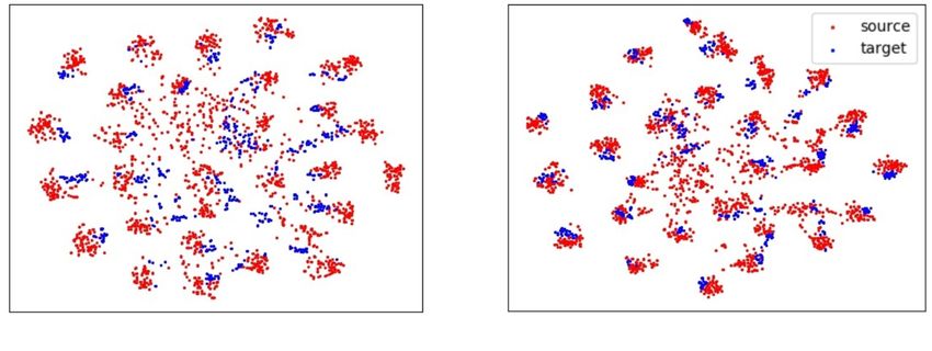
Feature visualization: To visually examine the effectiveness of the proposed method, we compare
t-SNE embedding of the features [33] from ResNet-50 and our SFDA on A ⇒ W in Office-31. As
shown in Fig. 3(b), we can observe that the source and target domains are better aligned by SFDA.
7This result clearly shows that it is possible to mitigate the discrepancy between two different domains
without accessing source data.
Statistics of reliable samples: We treat samples with the entropy values less than 0.2 as “reliable
samples", which accounts for about 30% of total samples as shown in Fig. 1. Note that these statistics
can change as our SFDA evolves progressively during the training phase. Hence, we further analyze
the changes in these statistics as training progresses. From Fig. 4(a), we can observe the percentage of
“reliable samples" gradually increases and eventually exceeds 50% of total samples. More importantly,
the accuracy of pseudo-labels of reliable samples also increases.
APM update period: We update APM periodically to reflect the statistics of the target domain using
our progressively evolving target model. Figure 4(b) shows the performance of our method with
different APM update periods. The shorter the update period, the better the accuracy, but requires
a higher amount of computation during training. Conversely, increasing the update period (e.g.
over 1000) degrades performance as the target model cannot fully utilize its self-learning scheme.
Empirically, we set the update period to 100 across all the datasets.
Trade-off parameter α: We analyze the trade-off parameter α between the source-regularization
loss and the self-learning loss in Eq. (8) as shown in Fig. 4(c). In the experiment, we investigate
two strategies: static α and dynamic α. For static α, we vary the value from 0 to 1. Using only
source-regularization loss, i.e., α = 0, does not utilize the advantage of the updated target model,
so performance is lower than in other settings. On the other hand, relying solely on self-learning
loss, i.e., α = 1, may fall into local minima due to self-biasing. In SFDA, we set dynamic α with
a schedule, α = 2(1 + exp(−10 · iter/max_iter))−1 − 0.5), so that the target model is updated
gradually from the source model. From this experiment, we can observe that dynamic α outperforms
all settings of static α, which demonstrates the effectiveness of our dynamic scheduling.
4 Related work
Unsupervised domain adaptation (UDA): Early UDA methods exploit distribution matching to
alleviate the domain discrepancy between source and target domains. Tzeng et al.[34] introduce a
domain confusion loss using maximum mean discrepancy (MMD) [34, 26]. Subsequently, a number
of variants based on distribution matching have been proposed, e.g., JMMD [35, 35], CMD [36],
MCD [30]. Meanwhile, there has been a growing interest in domain adversarial methods [9]. In
these approaches, the domain discriminator is trained to predict the domain label from features,
and at the same time, the feature extractor tries to deceive the domain discriminator, resulting in
domain-invariant features. Due to its simple yet effective extensibility and outstanding results, domain
adversarial training has been widely used across various fields [37, 38, 12, 39]. Unfortunately, existing
UDA methods require labeled source data, which can lead to privacy issues. Instead of accessing the
source data directly, we perform domain adaptation by leveraging a pre-trained source model.
Fine-tuning: One of the most practical paradigms in deep learning-based approaches is transfer
learning. Especially, fine-tuning parameters of a pre-trained model on large-scale datasets [40, 41] to a
specific target task has shown promising results in various areas [42, 38, 43]. For instance, VGG [44]
or ResNet [2] trained from ImageNet [40] are extensively fine-tuned for smaller dataset such as
Pascal VOC [45, 46]. 3D CNN models trained from Kinetics [41] are also used for UCF101 [47]
and HMDB51 [48] by default. Furthermore, fine-tuning is widely applied in two different but highly-
related tasks, e.g., from image classification to object detection, and significantly outperforms a model
trained from scratch. Compared with the fine-tuning technique, our SFDA protocol yields a crucial
advantage of being free from labor-intensive labeling of the target domain.
Knowledge distillation (KD): Our SFDA is related to KD [49] in that there are two models in which
one model depends on the other. However, fundamentally, KD aims to transfer the knowledge of
a large model (teacher) to a small model (student), so both models use the same dataset. In other
words, there is generally no covariate shift [15] in KD. Several studies [50, 51, 52] have demonstrated
that the teacher model pre-trained from the source data can transfer knowledge to the student model
for the target domain. Despite promising results even in the presence of domain discrepancy, these
techniques all require the labeling of samples in the target domain. In contrast, the proposed SFDA
can transfer knowledge from a labeled source domain to an unlabeled target domain during training.
85 Conclusion
In this paper, we have proposed a novel paradigm shift for unsupervised domain adaption, called
Source data-Free Domain Adaptation (SFDA) from a source pre-trained model. Our main (target)
model utilizes a pre-trained model from the source domain instead of using source data directly.
Specifically, two types of pseudo labels are used for training our target model. Target-oriented
pseudo labels obtained from the adaptive prototype memory are used to train the target model in a
self-learning manner while source-oriented pseudo labels prevent the target model from a self-biasing
problem. Despite not directly accessing the source data, our model achieves higher performance than
conventional models trained with source data. From extensive empirical analysis for SFDA scenarios,
we claim that SFDA is one of the effective ways to address data-privacy issues caused by labeled data
with sensitive attributes. In this study, we address the closed-set domain adaptation scenario where
the class set of source and target is identical. But in real-world scenarios, the source and target class
set might be different and it could affect our class prototype selection scheme. As future work, we
plan to extend the proposed SFDA approach to more realistic openset and partial domain adaptation
scenarios. Also, we will perform SFDA on datasets that contain sensitive labels, e.g., bio-metric
information, and address the encountered issues.
Broader Impact
This study suggests a paradigm shift by addressing the data-privacy issue, especially in unsupervised
domain adaptation. Based on our source data-free method, various stakeholders including enterprises
and government organizations can be free of concern about privacy issues with their labeled source
dataset.
Furthermore, the proposed data-free approach can contribute to creating a positive social impact,
especially when the data is in large-scale. Recently, since the size of data across various fields has
been scaling up for model training, it is almost incapable for individual researchers, startups, and
small or medium enterprises to directly utilize such large scale of data during training. For this
reason, a new social trend of sharing pre-trained models, e.g., NasNet, EfficientNet, and BERT, led by
global enterprises with their huge amount of resources has been rising up. These efforts can provide
more opportunities for people to join AI community by participating AI-based research or related
large-scale projects. Our approach based on pre-trained models thus can create social impact by
proposing new as well as beneficial solution, so that more people can participate in domain adaptation
research specifically when the source data is large-scale and contains sensitive attributes.
On the other hand, our method potentially limits the degree of freedom when modifying or adding
source data, e.g., annotation, or data pre-processing, especially in the case of requiring/expecting
more flexible domain adaptation. In conclusion, we believe that SFDA proposes a new protocol in
domain adaptation and even suggests a potential solution for increasing the need for safety in data
privacy and data security.
Supplementary Material
Appendix (A): Reimplementation
In our experiments, we compare the proposed method with the previous UDA methods. Importantly,
early UDA methods report performance based on Caffe while recent works are based on Pytorch
implementation. Therefore, the performance of early works tends to be considerably lower than the
recent works including ours. For a fair comparison, we re-implement ResNet-50, DAN, DANN, and
MSTN (DANN-based) using Pytorch.
Experimental setup: We use a batch size of 32 across all the datasets. Also, we set the maximum
iteration step to 10,000 for Office-31, 20,000 for Office-Home. We use SGD as the optimizer with
a weight decay of 0.0005 and a momentum of 0.9. The base learning rate is set to 10−3 and all
fine-tuned layers in a pre-trained feature extractor are optimized with a learning rate of 10−4 . We
apply a learning rate schedule with lrp = lr0 (1 + α · p)−β where lr0 is a base learning rate, p is a
relative step that changes from 0 to 1 during training, α = 10, and β = 0.75.
9In Table 4 and Table 5, we compare the performance between reported accuracy (Caffe) [29, 10]
and our reimplementation (Pytorch). The results show that our re-implemented results achieve
higher performance than the previously reported results, especially for ResNet baseline. For a fair
comparison, we reimplement early UDA methods using Pytorch and compare them with the proposed
method in our main paper.
Table 4: Classification Accuracy (%) on Office-31 (ResNet-50)
Office-31
Method
A⇒W D⇒W W⇒D A⇒D D⇒A W⇒A Avg
ResNet (reported) 68.4 ± 0.2 96.7 ± 0.1 99.3 ± 0.1 68.9 ± 0.2 62.5 ± 0.3 60.7 ± 0.3 76.1
DAN (reported) 80.5 ± 0.4 97.1 ± 0.2 99.6 ± 0.1 78.6 ± 0.2 63.6 ± 0.3 62.8 ± 0.2 80.4
DANN (reported) 82.0 ± 0.4 96.9 ± 0.2 99.1 ± 0.1 79.7 ± 0.4 68.2 ± 0.4 67.4 ± 0.5 82.2
ResNet 79.8 ± 0.6 98.3 ± 0.3 99.9 ± 0.1 83.8 ± 0.5 66.1 ± 0.3 65.1 ± 0.2 82.2
DAN 82.6 ± 0.6 98.5 ± 0.1 100.0 ± .0 83.6 ± 0.5 67.3 ± 0.8 66.3 ± 0.4 83.1
DANN 84.8 ± 0.9 98.2 ± 0.3 99.9 ± 0.1 86.3 ± 0.8 68.9 ± 0.4 66.8 ± 0.6 84.1
Table 5: Classification Accuracy (%) on Office-Home (ResNet-50)
Office-Home
Method
Ar⇒Cl Ar⇒Pr Ar⇒Rw Cl⇒Ar Cl⇒Pr Cl⇒Rw Pr⇒Ar Pr⇒Cl Pr⇒Rw Rw⇒Ar Rw⇒Cl Rw⇒Pr Avg
ResNet (reported) 34.9 50.0 58.0 37.4 41.9 46.2 38.5 31.2 60.4 53.9 41.2 59.9 46.1
DAN (reported) 43.6 57.0 67.9 45.8 56.5 60.4 44.0 43.6 67.7 63.1 51.5 74.3 56.3
DANN (reported) 45.6 59.3 70.1 47.0 58.5 60.9 46.1 43.7 68.5 63.2 51.8 76.8 57.6
ResNet 42.5 65.8 74.1 57.4 63.7 67.7 55.7 39.1 72.9 66.1 46.3 76.9 60.7
DAN 45.4 65.8 73.9 56.9 61.4 65.9 56.1 43.0 73.2 67.5 50.4 78.5 61.5
DANN 45.7 66.6 73.4 58.0 64.9 68.3 55.9 42.6 74.1 66.5 49.7 77.5 62.0
Appendix (B): Additional ablation on VisDA-C
We perform the ablation analysis regarding a trade-off parameter α on VisDA-C. A detailed description
of the experimental protocol is described in Section 3.3 in our main paper. As reported in Table 6, we
investigate two strategies: static α = [0.0, 0.2, 0.4, 0.6, 0.8, 1.0] and dynamic α = 2(1 + exp(−10 ·
iter/max_iter))−1 − 0.5). From the table, we can observe similar results as in Office-31. Using
only source-regularization loss (α = 0) or self-learning loss (α = 1) degrades performance since they
rely on one-sided information (source or target). Although using both source and target information
shows promising results in the static setting, dynamic α outperforms all the settings of static α.
Table 6: Classification Accuracy (%) on Visda-C (ResNet-101)
Vidsa-C
Method
aero bicycle bus car horse knife motor person plant skate train train Avg
SFDA (α = 0.0) 87.1 66.7 73.4 56.2 91.1 43.9 83.3 57.8 76.8 53.1 84.7 43.0 68.1
SFDA (α = 0.2) 87.9 70.0 80.5 63.8 92.2 66.1 87.9 65.0 78.3 56.9 78.0 46.6 72.8
SFDA (α = 0.4) 88.5 75.2 81.9 62.7 91.5 82.3 88.0 68.8 81.9 62.3 77.4 44.5 75.4
SFDA (α = 0.6) 86.5 74.8 81.2 61.0 90.4 90.8 84.7 77.6 75.9 52.7 78.2 47.7 75.1
SFDA (α = 0.8) 85.5 77.0 84.4 62.9 91.8 89.6 81.8 76.4 78.4 54.6 76.5 32.3 74.3
SFDA (α = 1.0) 86.8 81.2 86.5 60.6 90.7 91.3 82.3 69.5 81.5 51.6 73.0 37.6 74.4
SFDA (dynamic α ) 86.9 81.7 84.6 63.9 93.1 91.4 86.6 71.9 84.5 58.2 74.5 42.7 76.7
Appendix (C): Confidence-base filtering
In this section, we introduce Hausdorff distance (Eq. 3) in Confidence-base filtering in more detail. The
objective of confidence-base filtering is to estimate the confidence of a pseudo label by considering
the corner cases between two sets. Here, we compute the relationship of three sets as following:
• Q: a singleton set containing embedded feature of sample xt , i.e., {ft }.
• Mt1 : a set containing multiple prototypes of the most similar class (defined by sc (xt ) in Eq. 2).
• Mt2 : a set containing multiple prototypes of the second similar class.
10The Hausdorff distance can be formulated as follows:
dH (Q, Mt1 ) = max sup inf d(q, p), sup inf d(q, p)
q∈Q p∈Mt1 p∈Mt1 q∈Q
= max max min d(q, p), max min d(q, p) (9)
q∈Q p∈Mt1 p∈Mt1 q∈Q
= max min d(ft , p), max d(ft , p) = max d(ft , p).
p∈Mt1 p∈Mt1 p∈Mt1
In the second line, since Q, Mt1 , and Mt2 are closed and discretized sets, we can convert the suprema
and infima to maxima and minima, respectively. In the third line, since Q is a singleton set, i.e., ft is
the only element in the set, we can simplify max and min by inserting ft to q.
In the similar way, for the second most similar class, we slightly modify Hausdorff distance to select
the opposite corner case as follows:
∗
dH (Q, Mt2 ) = min sup inf d(q, p), sup inf d(q, p)
q∈Q p∈Mt2 p∈Mt2 q∈Q
= min max min d(q, p), max min d(q, p) (10)
q∈Q p∈Mt2 p∈Mt2 q∈Q
= min min d(ft , p), max d(ft , p) = min d(ft , p).
p∈Mt2 p∈Mt2 p∈Mt2
References
[1] Ren, S., He, K., Girshick, R., Sun, J.: Faster r-cnn: Towards real-time object detection with
region proposal networks. In: Proc. of Neural Information Processing Systems (NeurIPS).
(2015) 91–99
[2] He, K., Zhang, X., Ren, S., Sun, J.: Deep residual learning for image recognition. In: Proc. of
Computer Vision and Pattern Recognition (CVPR). (2016) 770–778
[3] Chen, L.C., Papandreou, G., Kokkinos, I., Murphy, K., Yuille, A.L.: Deeplab: Semantic image
segmentation with deep convolutional nets, atrous convolution, and fully connected crfs. IEEE
Trans. on Pattern Anal. Mach. Intell. (TPAMI) 40(4) (2017) 834–848
[4] Hong, S., Kang, S., Cho, D.: Patch-level augmentation for object detection in aerial images. In:
Proceedings of the IEEE International Conference on Computer Vision Workshops. (2019) 0–0
[5] Cho, D., Hong, S., Kang, S., Kim, J.: Key instance selection for unsupervised video object
segmentation. arXiv preprint arXiv:1906.07851 (2019)
[6] Feichtenhofer, C., Fan, H., Malik, J., He, K.: Slowfast networks for video recognition. In: Proc.
of Int’l Conf. on Computer Vision (ICCV). (2019) 6202–6211
[7] Kim, Y., Kim, S., Kim, T., Kim, C.: Cnn-based semantic segmentation using level set loss. In:
Proc. of Winter Conf. on Applications of Computer Vision (WACV), IEEE (2019) 1752–1760
[8] Lee, H., Choi, S., Kim, Y., Kim, C.: Bilinear siamese networks with background suppression
for visual object tracking. In: Proc. of British Machine Vision Conf. (BMVC). (2019) 8
[9] Ganin, Y., Lempitsky, V.: Unsupervised domain adaptation by backpropagation. Proc. of Int’l
Conf. on Machine Learning (ICML) (2015) 1180–1189
[10] Long, M., Cao, Z., Wang, J., Jordan, M.I.: Conditional adversarial domain adaptation. In:
Advances in Neural Information Processing Systems. (2018) 1640–1650
[11] Hsu, H.K., Yao, C.H., Tsai, Y.H., Hung, W.C., Tseng, H.Y., Singh, M., Yang, M.H.: Progressive
domain adaptation for object detection. In: Proc. of Winter Conf. on Applications of Computer
Vision (WACV). (2020) 749–757
[12] Tsai, Y.H., Hung, W.C., Schulter, S., Sohn, K., Yang, M.H., Chandraker, M.: Learning to adapt
structured output space for semantic segmentation. In: Proc. of Computer Vision and Pattern
Recognition (CVPR). (2018) 7472–7481
11[13] Hong, S., Ryu, J.: Unsupervised face domain transfer for low-resolution face recognition. IEEE
Signal Process. Lett. (SPL) (2019)
[14] Choi, S., Lee, S., Kim, Y., Kim, T., Kim, C.: Hi-cmd: Hierarchical cross-modality disentan-
glement for visible-infrared person re-identification. In: Proc. of Computer Vision and Pattern
Recognition (CVPR). (2020) 10257–10266
[15] Sugiyama, M., Storkey, A.J.: Mixture regression for covariate shift. In: Proc. of Neural
Information Processing Systems (NeurIPS). (2007) 1337–1344
[16] HUAWEI: AI Security White Paper. (2018)
[17] Woodard, D.L., Pundlik, S.J., Lyle, J.R., Miller, P.E.: Periocular region appearance cues for
biometric identification. In: CVPRW, IEEE (2010) 162–169
[18] Naderi, H., Soleimani, B.H., Matwin, S., Araabi, B.N., Soltanian-Zadeh, H.: Fusing iris,
palmprint and fingerprint in a multi-biometric recognition system. In: Conf. on Computer and
Robot Vision (CRV), IEEE (2016) 327–334
[19] Nagrani, A., Albanie, S., Zisserman, A.: Seeing voices and hearing faces: Cross-modal biometric
matching. In: Proc. of Computer Vision and Pattern Recognition (CVPR). (2018) 8427–8436
[20] Bae, J.K., Kim, J.: A personal credit rating prediction model using data mining in smart
ubiquitous environments. Int’l Journal of Distributed Sensor Networks 11(9) (2015) 179060
[21] Smith, V., Chiang, C.K., Sanjabi, M., Talwalkar, A.S.: Federated multi-task learning. In: Proc.
of Neural Information Processing Systems (NeurIPS). (2017) 4424–4434
[22] Yang, Q., Liu, Y., Chen, T., Tong, Y.: Federated machine learning: Concept and applications.
Trans. on Intelligent Systems and Technology (TIST) 10(2) (2019) 1–19
[23] Saenko, K., Kulis, B., Fritz, M., Darrell, T.: Adapting visual category models to new domains.
In: Proc. of European Conf. on Computer Vision (ECCV), Springer (2010) 213–226
[24] Venkateswara, H., Eusebio, J., Chakraborty, S., Panchanathan, S.: Deep hashing network for
unsupervised domain adaptation. In: Proc. of Computer Vision and Pattern Recognition (CVPR).
(2017) 5018–5027
[25] Peng, X., Usman, B., Kaushik, N., Hoffman, J., Wang, D., Saenko, K.: Visda: The visual domain
adaptation challenge. arXiv preprint arXiv:1710.06924 (2017)
[26] Long, M., Cao, Y., Wang, J., Jordan, M.I.: Learning transferable features with deep adaptation
networks. Proc. of Int’l Conf. on Machine Learning (ICML) (2015) 97–105
[27] Xie, S., Zheng, Z., Chen, L., Chen, C.: Learning semantic representations for unsupervised
domain adaptation. In: Proc. of Int’l Conf. on Machine Learning (ICML). (2018) 5423–5432
[28] Pei, Z., Cao, Z., Long, M., Wang, J.: Multi-adversarial domain adaptation. In: Thirty-Second
AAAI Conference on Artificial Intelligence. (2018)
[29] Xu, R., Li, G., Yang, J., Lin, L.: Larger norm more transferable: An adaptive feature norm
approach for unsupervised domain adaptation. In: Proceedings of the IEEE International
Conference on Computer Vision. (2019) 1426–1435
[30] Saito, K., Watanabe, K., Ushiku, Y., Harada, T.: Maximum classifier discrepancy for unsuper-
vised domain adaptation. In: Proc. of Computer Vision and Pattern Recognition (CVPR). (2018)
3723–3732
[31] Chang, W.G., You, T., Seo, S., Kwak, S., Han, B.: Domain-specific batch normalization for
unsupervised domain adaptation. In: Proc. of Computer Vision and Pattern Recognition (CVPR).
(2019) 7354–7362
[32] Deng, J., Dong, W., Socher, R., Li, L.J., Li, K., Fei-Fei, L.: Imagenet: A large-scale hierarchical
image database. In: Proc. of Computer Vision and Pattern Recognition (CVPR), Ieee (2009)
248–255
[33] Maaten, L.v.d., Hinton, G.: Visualizing data using t-sne. Journal of Machine Learning Research.
(JMLR) 9(Nov) (2008) 2579–2605
[34] Tzeng, E., Hoffman, J., Zhang, N., Saenko, K., Darrell, T.: Deep domain confusion: Maximizing
for domain invariance. arXiv preprint arXiv:1412.3474 (2014)
12[35] Long, M., Zhu, H., Wang, J., Jordan, M.I.: Unsupervised domain adaptation with residual
transfer networks. In: Proc. of Neural Information Processing Systems (NeurIPS). (2016)
136–144
[36] Zellinger, W., Grubinger, T., Lughofer, E., Natschläger, T., Saminger-Platz, S.: Central moment
discrepancy (cmd) for domain-invariant representation learning. (2017)
[37] Bousmalis, K., Trigeorgis, G., Silberman, N., Krishnan, D., Erhan, D.: Domain separation
networks. In: Proc. of Neural Information Processing Systems (NeurIPS). (2016) 343–351
[38] Tzeng, E., Hoffman, J., Saenko, K., Darrell, T.: Adversarial discriminative domain adaptation.
In: Proc. of Computer Vision and Pattern Recognition (CVPR). (2017) 7167–7176
[39] Hong, S., Ryu, J.: Attention-guided adaptation factors for unsupervised facial domain adaptation.
Electronics Letters (2020)
[40] Russakovsky, O., Deng, J., Su, H., Krause, J., Satheesh, S., Ma, S., Huang, Z., Karpathy, A.,
Khosla, A., Bernstein, M., Berg, A.C., Fei-Fei, L.: ImageNet Large Scale Visual Recognition
Challenge. Int’l Journal of Computer Vision (IJCV) 115(3) (2015)
[41] Kay, W., Carreira, J., Simonyan, K., Zhang, B., Hillier, C., Vijayanarasimhan, S., Viola, F.,
Green, T., Back, T., Natsev, P., Suleyman, M., Zisserman, A.: The kinetics human action video
dataset. CoRR abs/1705.06950 (2017)
[42] Karpathy, A., Fei-Fei, L.: Deep visual-semantic alignments for generating image descriptions.
In: Proc. of Computer Vision and Pattern Recognition (CVPR). (2015) 3128–3137
[43] Radenović, F., Tolias, G., Chum, O.: Fine-tuning cnn image retrieval with no human annotation.
IEEE Trans. on Pattern Anal. Mach. Intell. (TPAMI) 41(7) (2018) 1655–1668
[44] Simonyan, K., Zisserman, A.: Very deep convolutional networks for large-scale image recogni-
tion. (2015)
[45] Everingham, M., Van Gool, L., Williams, C.K.I., Winn, J., Zisserman, A.: The PAS-
CAL Visual Object Classes Challenge 2007 (VOC2007) Results. http://www.pascal-
network.org/challenges/VOC/voc2007/workshop/index.html (2007)
[46] Everingham, M., Van Gool, L., Williams, C.K.I., Winn, J., Zisserman, A.: The PAS-
CAL Visual Object Classes Challenge 2012 (VOC2012) Results. http://www.pascal-
network.org/challenges/VOC/voc2012/workshop/index.html (2012)
[47] Soomro, K., Zamir, A.R., Shah, M.: Ucf101: A dataset of 101 human actions classes from
videos in the wild. arXiv preprint arXiv:1212.0402 (2012)
[48] Kuehne, H., Jhuang, H., Garrote, E., Poggio, T., Serre, T.: HMDB: a large video database for
human motion recognition. In: Proc. of Int’l Conf. on Computer Vision (ICCV). (2011)
[49] Hinton, G., Vinyals, O., Dean, J.: Distilling the knowledge in a neural network. In: In: Proc. of
Neural Information Processing Systems (NeurIPS) Deep Learning and Representation Learning
Workshop. (2015)
[50] Zagoruyko, S., Komodakis, N.: Paying more attention to attention: Improving the performance
of convolutional neural networks via attention transfer. (2017)
[51] Srinivas, S., Fleuret, F.: Knowledge transfer with Jacobian matching. In: Proc. of Int’l Conf. on
Machine Learning (ICML). (2018) 4723–4731
[52] Heo, B., Lee, M., Yun, S., Choi, J.Y.: Knowledge transfer via distillation of activation boundaries
formed by hidden neurons. (2019)
13You can also read