Wobbling double sine-Gordon kinks
←
→
Page content transcription
If your browser does not render page correctly, please read the page content below
Published for SISSA by        Springer
                                                                    Received: March 10,    2021
                                                                      Revised: August 6,   2021
                                                                   Accepted: August 22,    2021
                                                                Published: September 10,   2021

Wobbling double sine-Gordon kinks

                                                                                                  JHEP09(2021)067
João G.F. Campos1 and Azadeh Mohammadi2
 Departamento de Física, Universidade Federal de Pernambuco,
 Av. Prof. Moraes Rego, 1235, Recife – PE – 50670-901, Brazil

 E-mail: joao.gfcampos@ufpe.br, azadeh.mohammadi@ufpe.br

Abstract: We study the collision of a kink and an antikink in the double sine-Gordon
model with and without the excited vibrational mode. In the latter case, we find that
there is a limited range of the parameters where the resonance windows exist, despite the
existence of a vibrational mode. Still, when the vibrational mode is initially excited, its
energy can turn into translational energy after the collision. This creates one-bounce as
well as a rich structure of higher-bounce resonance windows that depend on the wobbling
phase being in or out of phase at the collision and the wobbling amplitude being sufficiently
large. When the vibrational mode is excited, the modified structure of one-bounce windows
is observed in the whole range of the model’s parameters, and the resonant interval with
higher-bounce windows gradually increases with the wobbling amplitude. We estimated
the center of the one-bounce windows using a simple analytical approximation for the
wobbling evolution. The kinks’ final wobbling frequency is Lorentz contracted, which is
simply derived from our equations. We also report that the maximum energy density value
always has a smooth behavior in the resonance windows.

Keywords: Solitons Monopoles and Instantons, Field Theories in Lower Dimensions

ArXiv ePrint: 2103.04908

  1
      https://orcid.org/0000-0002-1723-4562.
  2
      https://orcid.org/0000-0001-5720-7086.

Open Access, c The Authors.
                                                    https://doi.org/10.1007/JHEP09(2021)067
Article funded by SCOAP3 .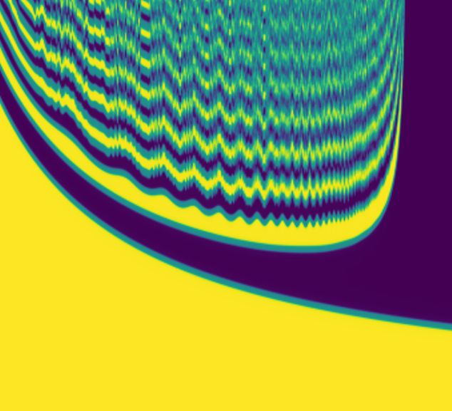
Contents

1 Introduction                                                                                 1

2 Model                                                                                        3

3 Collision simulations                                                                        5

4 Conclusion                                                                                  13

                                                                                                    JHEP09(2021)067
A Numerical technique                                                                         15

1   Introduction

Solitons, instantons and monopoles for instance, are important solutions of field theories
that appear when the configuration of the system at the boundary is topologically non-
trivial [1, 2]. In particular, soliton solutions of relativistic scalar field theories in (1 + 1)
dimensions are called kink and antikink. The degeneracy of the potential is essential for
their existence. These solutions appear in the description of many physical systems such
as polyacetylene [3], Josephson junctions [4], graphene deformations [5], domain walls in
ferromagnets [6] and Helium-3 [7].
     Two of the most studied models in the field are the sine-Gordon and the φ4 . The
sine-Gordon is integrable, giving rise to what is called a true soliton. The φ4 , on the other
hand, is non-integrable and exhibits a much wider variety of outcomes. In the former,
the collision between the kinks is always elastic, and the only effect of the interaction is
a phase shift in the kinks propagation. In the latter, the constituents in a kink-antikink
collision may instead reflect inelastically or annihilate. Moreover, it may also happen that
the solitons separate after more than one-bounce in what is called resonance windows.
This interesting phenomenon has been extensively studied for a few decades and had no
compelling quantitative explanation until recently [8, 9].
     Historically, the pioneering works about kink-antikink collisions include Sugiyama [10],
Campbell et al. [11–13]. and Anninos et al. [14]. In [10], the author observed that, after
the collision, a kink and an antikink annihilate or reflect after a critical velocity. Moreover,
the author proposed a reduced model describing the system using collective coordinates.
Unfortunately, one of the equations had a typo that propagated in the literature for many
years. In the triplet of papers [11–13] the authors computed the resonance windows for the
φ4 model, a modified sine-Gordon model, and the double sine-Gordon with high precision.
Moreover, they argued that the resonance windows occur due to a resonant energy exchange
mechanism between the kink’s translational and vibrational modes. Thus, they found an-
alytical expressions for the windows’ location and shape and conjectured that higher-order

                                             –1–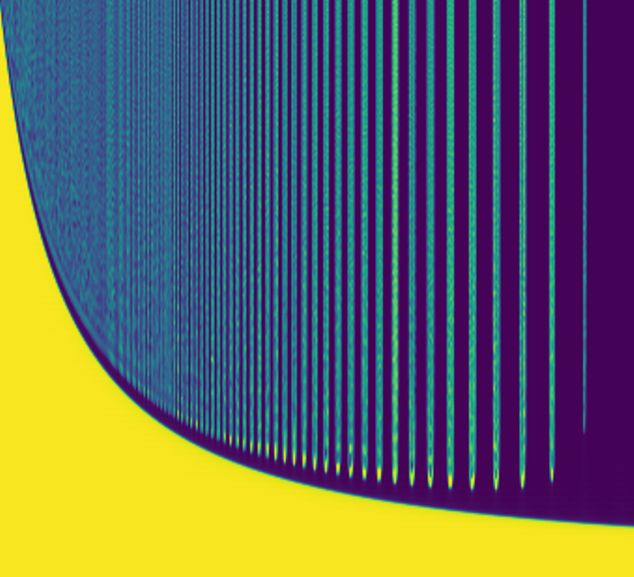
resonance windows exist at the border of the lower-order ones. In [14] the authors showed
that resonance windows form a fractal structure, both numerically and using the reduced
system proposed by Sugiyama. Unfortunately, when the typo in the reduced equations was
corrected, the qualitative similarity between the reduced and full systems disappeared [15].
To remedy that, the authors of [15] tried to integrate the reduced equations without any
approximation but faced a singularity in the equations. Finally, in two recent works, this
singularity problem was corrected with a clever choice of collective coordinates [8], and
then the reduced equations could reproduce the resonance structure [9].
     There has been a great number of works discussing kink-antikink interactions in various
scenarios in the literature. Some of these include the investigation of quasinormal modes in

                                                                                                 JHEP09(2021)067
kink-antikink collisions [16, 17], models with BPS preserving defects [18–23], interactions of
kinks with fermions [24–28], collisions between kinks with long-range tails [29–34], collision
of kinks with boundaries [35–37], multikink scattering [38–41] and collision between kinks
in two-component scalar field theories [42–44].
     The double sine-Gordon model is a compelling non-integrable model which becomes
integrable in some limits. Therefore, it is possible to study a gradual transition from
integrability to non-integrability. Early works of the double sine-Gordon model studied
it as a perturbation of the sine-Gordon model via the inverse scattering method [45–47].
However, to leading order, a conservative perturbation to the sine-Gordon model still has
a trivial kink-antikink collision [47]. Other important works about kink collisions in this
model include [13, 41, 48–50]. An important feature that appears in these works is that
the kinks have an inner structure, i.e., it consists of two subkinks, which may be exchanged
at collision and form subkink bound states. This phenomenon was also observed in other
systems with the kinks with inner structures [51]. Curiously, the double sine-Gordon model
may effectively describe some physical systems such as gold dislocations [52], optical pulses
and spin waves [53], pseudo 1-D ferromagnets [54] and Josephson structures [55]. Despite
all that, it has not been sufficiently explored in the literature. It was only recently that
the dependence of the critical velocity on the model parameter R was calculated [49].
     Recently Alonso-Izquierdo et al. studied a fascinating problem for kink-antikink inter-
actions [56]. They considered collisions between wobbling kinks, meaning that the kinks
have their vibrational mode excited at the collision. A single wobbling kink’s behavior has
already been studied for the φ4 model [57–59]. In particular, it is well known that the
wobbling amplitude decreases due to coupling to radiation via the first harmonic [57] or,
for some other models, via higher harmonics [60]. The collision between wobbling kinks
is important because the successive bounces in resonance windows may be seen as an it-
eration of such events. Interestingly, the authors showed in [56] that there appear many
separate one-bounce windows due to the wobbling. Here, we study collisions between wob-
bling double sine-Gordon kink and antikink. Interestingly, when the wobbling is turned
off, the model does not exhibit resonance windows near its integrable limits, despite hav-
ing a vibrational mode. This seems to be an exception to the resonant energy exchange
mechanism. However, when the wobbling is turned on, the resonant structure is gradu-
ally recovered. We show that the double sine-Gordon shares many similar features with
the φ4 model, such as one-bounce resonance windows. We are able to approximate the

                                            –2–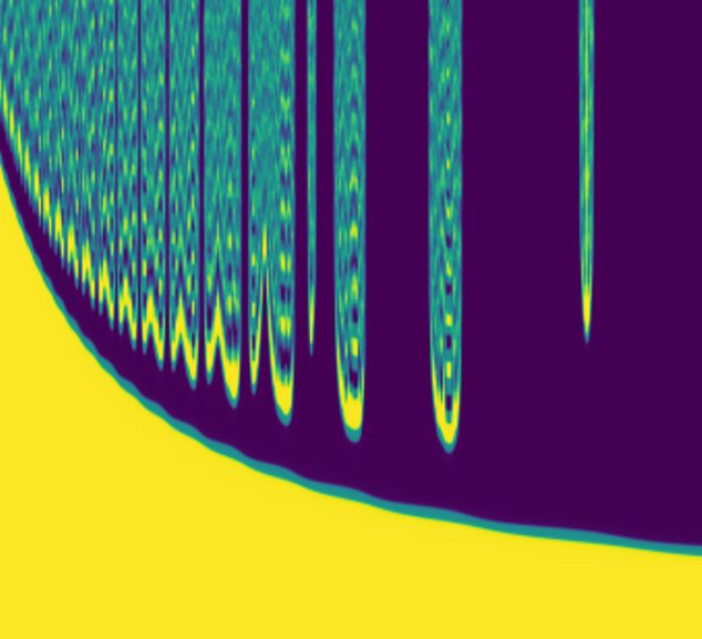
(a)                                                  (b)                                          (c)

                                                           6       R = 0.5                                  1.00
     6
                                                                   R = sinh−1 (1)
                                                                                                            0.75
                                                           4       R = 1.4
     5
                                                                   R = 3.0                                  0.50

     4                                                     2
                                                                                                            0.25

                                                                                                      UR
VR

                                                     φk
     3                                                     0                                                0.00

                                                                                                           −0.25
     2                                                    −2
                                                                                                           −0.50
     1                                                    −4
                                                                                                           −0.75

     0                                                    −6
                                                                                                           −1.00

                                                                                                                                              JHEP09(2021)067
         −4π −3π −2π −π   0     π    2π   3π   4π                  −5           0             5                        −5   0     5
                          φ                                                     x                                           x

Figure 1. (a) Potential, (b) kink profile, and (c) linearized potential for the double sine-Gordon
model with different values of the parameter R.

locations of these windows using the simplified analysis of the resonance windows structure
of Campbell et al. Furthermore, this can also be visualized by plotting the maximum value
of the energy densities similar to the analysis in [41, 61]. The structure of the paper is as
follows. In section 2 we give a brief review of the double sine-Gordon models. In section 3
we show and compare the numerical results of our simulations of kink-antikink collisions
with and without wobbling. Finally, in the last section, we give our concluding remarks.

2         Model

Let us consider the double sine-Gordon model described by the following Lagrangian in
(1 + 1) dimensions
                                       1
                                   L = (∂µ φ)2 − VR (φ),                         (2.1)
                                       2
where φ is a scalar field and the potential term is given by [13]
                                                                                         4            φ

                                    VR (φ) = tanh2 R(1 − cos φ) +                             1 + cos   .                             (2.2)
                                                                                      cosh2 R         2
The potential is periodic and is shown in figure 1(a) for some values of R. It is clear from
eq. (2.2) that for R = 0 and in the limit R → ∞ the potential approaches the sine-Gordon
one with periods 4π and 2π, respectively. For sinh−1 (1) ≤ R ≤ 0, the potential has only one
maximum per period, as in the sine-Gordon model. On the other hand, for R > sinh−1 (1),
a local minimum appears, which approaches zero in the large R limit.
     Solving the equation of motion of the system gives the following kink and antikink
solutions (see figure 1(b))
                                                                                              sinh x

                                                                                     −1
                                                    φk(k̄) = 4πn ± 4 tan                             ,                                (2.3)
                                                                                              cosh R
when the scalar field is static.                               If we write the sine-Gordon kink solution as φSG =
4 tan−1 exp(x), this becomes

                                           φk(k̄) = 4πn ± [φSG (x + R) − φSG (R − x)].                                                (2.4)

                                                                         –3–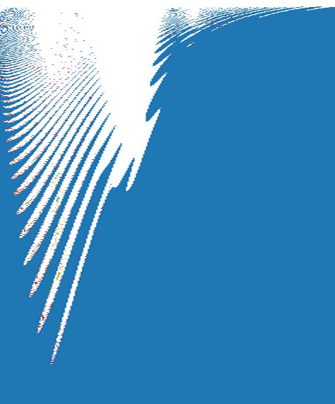
1.0

                                0.8

                                0.6

                           ωD
                            2
                                0.4

                                0.2

                                                                                                      JHEP09(2021)067
                                0.0

                                      0   1     2       3     4      5
                                                    R

Figure 2. Spectrum of the linearized equation around a kink solution. The solid line is the vibra-
tional mode, and the dashed line is the zero mode. The blue region represents the continuum region.

Therefore, one may interpret the double sine-Gordon kink as a superposition of two sine-
Gordon kinks separated by a distance of 2R.
    We are interested in collisions between double sine-Gordon kinks that are vibrating.
This is important to gain a deeper insight into the vibrational or shape modes’ role in
the resonance windows. Therefore, we look for these modes in the stability equation of
the kink solution. Writing φ = φk + ψeiωt , where ψ is a small perturbation, leads to the
Schrödinger-like equation
                                    − ψ 00 + UR ψ = ω 2 ψ,                          (2.5)
where the linearized stability potential is given by [49]

                            8 tanh2 R              2(3 − 4 cosh2 R)
               UR =                         +                             + 1.               (2.6)
                      (1 + sech2 R sinh2 x)2 cosh2 R(1 + sech2 R sinh2 x)
The potential is shown in figure 1(c) for several values of R. For large R, it clearly splits
into two sine-Gordon wells.
     The spectrum of the linearized equation as a function of R is shown in figure 2. It
contains a zero mode, as required by translational invariance, and a single vibrational
mode. The normalized profile of the shape mode is denoted by ψD with eigenvalue ωD        2.

It is simple to show that the energy stored in the shape mode with amplitude A is equal
to ED = 12 ωD 2 A2 . There is also a continuum of states starting at ω 2 = 1. For R = 0

the vibrational mode disappears in the continuum, as the kink solution becomes the sine-
Gordon one. For R  1 the value of ωD    2 approaches zero as the kink tends to two well-

separated sine-Gordon kinks.
     Before delving into the kink-antikink collision, let us first discuss the behavior of a
single wobbling kink. We start with a single excited kink at the origin, and we integrate
the equations of motion as described in appendix A. It is known that a vibrating kink decays
through the coupling to radiation, due to higher-order terms of the wobbling amplitude

                                              –4–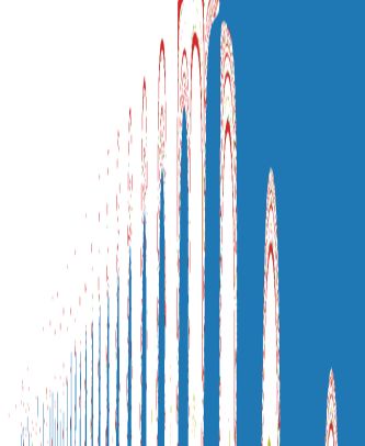
(c) R = 0.5                             (d) R = 1.0
                                             (a)                                                    ω1      2ω1 3ω1 4ω1                       ω1 2ω1 3ω1 4ω1
φ(∆x) − φk (∆x)

            0.45                                                                                                                    102
                                                                                       101

                                                                              |S(ω)|

                                                                                                                           |S(ω)|
            0.40
                                                                                                                                    100
            0.35
                                                                                  10−2
                                                                                                                               10−2
                          0        500       1000           1500       2000
                                               t                                             0       1       2     3   4                  0    1        2    3   4
                                             (b)                                                             ω                                          ω
                                                                                                         (e) R = 1.8                               (f) R = 2.1
                                                                                                 ω1 · · · 4ω1                             ω1 · · ·4ω1
            0.75
ω

                                                                                       102                                          102
            0.50

                                                                              |S(ω)|

                                                                                                                           |S(ω)|

                                                                                                                                                                     JHEP09(2021)067
                                                                                       100                                          100
                          0         500       1000          1500       2000
                                                                                                                               10−2
                                                t                                 10−2
                                  R = 0.5         R = 1.8          R = 2.1
                                  R = 1.0                                                    0       1      2     3    4                  0    1     2      3    4
                                                                                                            ω                                        ω

Figure 3. Evolution of the (a) amplitude and (b) frequency of oscillation of the shape mode at
∆x = 1.465. (c)-(f) Absolute value of the Fourier transform of the data from (a) and (b), considering
t > 1000. The purple line corresponds to the shape mode vibration at x = ∆x and the gray line to
the far-field vibration at x = 25.0. The initial amplitude is A = 1.0.

in the equations of motion, via the harmonics of the wobbling frequency. In the double
sine-Gordon model, the decay also follows the Manton-Merabet pattern [57] as shown in
figure 3 for R = 0.5 and R = 1.0. However, interestingly, the decay for R = 0.5 is much
less pronounced, and this phenomenon becomes more evident approaching the integrable
limit. Moving to higher values of R, we reach a point where the shape mode frequency
becomes lower than the half-threshold value. In this case, the decay occurs through higher
harmonics [60], as can be seen in the right panels. There, we take the Fourier transform
S(ω) of the field time series near the wobbling kink and far from it and plot its absolute
value. We see that the far-field spectrum, which corresponds to the emitted radiation, has
peaked in the harmonics of the vibration frequency above the continuum threshold. For
R = 1.8 and R = 2.1, the decay occurs mainly through the second and third harmonic,
respectively, and, therefore, the perturbation is much more stable [60], as can be seen in
the amplitude evolution.

3                     Collision simulations

To initialize the collision we take the following configuration

                        φ = φk (ξ+ ) − φk (ξ− ) − 2π + A sin(ωD τ+ )ψD (ξ+ ) − A sin(ωD τ− )ψD (ξ− ) ,                                                      (3.1)

evaluated at t = 0. For the time evolution we defined
                                                    q      the boosted coordinates ξ± =
                                      1
γ(x ± x0 ∓ vi t) and τ± = γ(t ∓ vi x), where γ = 1/ 1 − vi2 . It consists of a kink and an
antikink separated by a distance 2x0 , fixed at the value 2x0 = 30. They approach each
                  1
                      It is a common mistake to only impose the boost on x coordinate and neglect it in the time coordinate.

                                                                        –5–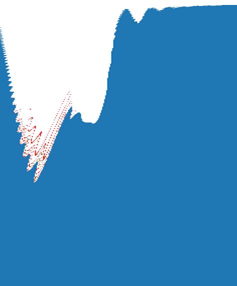
(a)                                                                       (b)
     0.6                                                                                                0.40
             0.25

             0.20                                                                                       0.35
     0.5
             0.15                                                                                       0.30
     0.4
             0.10                                                                                       0.25

             0.05
vf

     0.3                                                                                                0.20

                                                                                                   vi
             0.00                                                               1 bounce
                    0.20     0.22         0.24                                                          0.15
     0.2                                                                        2 bounces
                                                                                3 bounces               0.10
                                                                                4 bounces
     0.1
                                                                                5 bounces               0.05
                                                                                >5 bounces

                                                                                                                                                 JHEP09(2021)067
     0.0                                                                                                0.00
           0.0         0.1          0.2           0.3         0.4         0.5                0.6               0   1   2         3   4       5
                                                   vi                                                                      R

Figure 4. (a) Final velocity as a function of the initial velocity for kink-antikink collisions, con-
sidering R = 1.0. (b) Number of bounces before escape for kink-antikink collisions as a function of
the initial velocity vi and R. For both diagrams, we set A = 0.0.

other with velocity vi and −vi , respectively, and at the same time, they wobble with the
bound frequency ωD   2 and amplitude A. For A = 0, this leads to the usual kink-antikink

collision [13]. The technical details of the simulations are described in appendix A.
     From eq. (3.1), it is clear that the wobbling oscillation frequency is Lorentz contracted
in the center of mass frame. If we measure the time evolution of the field at a point moving
with the kink in the form x = vi t + α, the wobbling term becomes

                                                        ωD

                                          A sin            t − γωD vi α ψD (γ(x0 + α)),                                                  (3.2)
                                                         γ

which oscillates with a Lorentz contracted frequency ωD /γ. This transverse Doppler effect
was also shown to appear in a more detailed description of wobbling kinks investigated
in [58]. We will observe the same effect after the collision, where the frequency is contracted
according to the system’s final velocity.
     The double sine-Gordon model with A = 0 exhibits resonance windows in a finite range
of the parameter R. This occurs presumably because, for both very small and very large R,
the model becomes the sine-Gordon one, which is integrable and does not have resonance
windows. We show the final velocity as a function of the initial velocity for a specific value
of R = 1.0 in figure 4(a). This value is in the region where the system exhibits resonance
windows. The fractal structure is similar to the φ4 model. However, there is a significant
difference. Due to the periodicity of the potential, the kink and the antikink may either
cross or reflect. An even number of bounces means that the kinks reflected, while an odd
number means that the kinks crossed.
     In figure 4(b), we show the number of bounces as a function of R and vi , the initial
velocity of the incoming kink-antikink. The colors represent the number of bounces as
indicated in figure 4(a). The white region is where the kink and the antikink annihilate. In
the blue region, separation occurs after a single bounce. The interface between white and
blue determines the critical velocity value, which agrees with the non-monotonic behavior

                                                                    –6–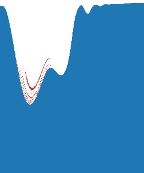
(a) R = 0.3, A = 0.0 φ0 (b) R = 3.0, A = 0.0 φ0
1400 1400
5 5
1200 1200
0 0
1000 1000
800 −5 800 −5
t
t
600 600
−10 −10
400 400
200 −15 200 −15
JHEP09(2021)067
0 0
0.010 0.015 0.020 0.025 0.030 0.035 0.040 0.045 0.050 0.010 0.015 0.020 0.025 0.030
vi vi
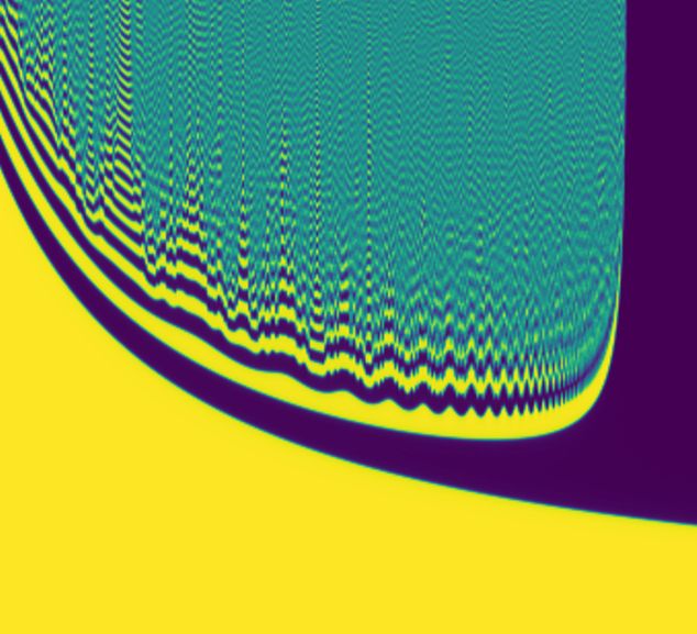
Figure 5. The value of the field at the center of collision as a function of time and the initial velocity.
reported in [49]. Moreover, the resonance domain with a fractal structure, the region
with dots in red and other colors, is located approximately in the interval 0.52 ≤ R ≤
1.78. This interval translates to a frequency interval 0.437 < ωD < 0.963. Of course, the
actual resonance domain would be slightly larger because the resonance windows become
increasingly narrower and consequently more difficult to locate.
To confirm that the model does not have resonance windows for large and small R,
we plot the time evolution of the field at the collision center as a function of the initial
velocity. This is shown in figure 5 for R = 0.3 and R = 3.0. In both cases, we can
only see false resonance windows, despite the presence of a vibrational mode. It means
that the existence of the vibrational mode does not guarantee the appearance of a fractal
structure. Therefore, the vibrational mode is not sufficient for the resonant energy exchange
mechanism. In [50], the authors obtained a similar result near the integrable limit of a case
of the double sine-Gordon different from what is investigated here and, in [62], the authors
also found false resonance windows near the integrable regime of a deformed sine-Gordon
model. We searched carefully for resonance windows with precision ∆vi = 10−5 and no
resonance windows were found.
Now we would like to see how the result with A 6= 0 compares with the previous
one. We start with a small value of A = 0.1. The final velocity dependence on the initial
one is shown in figure 6(a) for R = 1.0. We observe that the blue crossing curve, which
indicates separation after one-bounce, now oscillates as we vary vi . This occurs because,
for different velocities, the phase of the wobbling at the collision varies. Before the collision,
the wobbling amplitude evolves approximately as
ωD
S(t) = A exp i t + θ0 , (3.3)
γ
where θ0 is an initial constant. Moreover, the collision occurs approximately at t = x0 /vi .
Therefore, the dependence of the phase θ at the collision on vi can be estimated as
q
ωD x0
θ= 1 − vi2 + θ0 . (3.4)
vi
–7–(a) (b)
0.6 0.40
0.25
0.35
0.5 0.20
0.15 0.30
0.4
0.10 0.25
0.05
vf
0.3 0.20
vi
0.00 1 bounce
0.18 0.20 0.22 0.24 0.26 0.15
0.2 2 bounces
3 bounces 0.10
4 bounces
0.1
5 bounces 0.05
>5 bounces
JHEP09(2021)067
0.0 0.00
0.0 0.1 0.2 0.3 0.4 0.5 0.6 1 2 3 4 5
vi R
Figure 6. (a) Final velocity as a function of the initial velocity for kink-antikink collisions, con-
sidering R = 1.0. (b) Number of bounces before escape for kink-antikink collisions as a function of
the initial velocity vi and R. For both diagrams, we set A = 0.1.
Crossing after one bounce always occurs after a critical velocity. However, the oscillation in
the amplitude, shown in eq. (3.3), causes the one-bounce crossing curve to split, creating
one or more isolated one-bounce windows. Near these windows, there appears a nested
structure of higher-bounce windows. The gap between the two one-bounce regions occurs
because, in this region, the wobbling is out of phase at the collision time. Similarly, it is also
possible to see oscillating behavior in some two-bounce windows. This novel phenomenon
was also observed in the collision between wobbling kinks of the φ4 model [56].
In figure 6(b), we summarize the behavior of the system for both dependences on R
and vi . One important detail is that in contrast with the case of A = 0, for small R it
becomes difficult to find the shape mode profile numerically with enough precision as it
approaches the continuum. That is the reason we have shown the figure starting with a
small nonzero R. It is possible to see that the one-bounce crossing region oscillates with
many spines in double sine-Gordon model, similar to what was described in [62].2 These
spines originate from the formation of one-bounce resonance windows as explained in detail
in [62]. In short, the formation of spines can be pictured by tracking how the one-bounce
windows appear, move and connect as we change R. Another interesting point is that the
wobbling energy is enough to create one-bounce windows even for the values of R where
there was no fractal structure in the absence of wobbling, A = 0.
For A = 0.1, the wobbling effect is small, while if we increase A, it becomes more
pronounced. Figure 7(a) shows the system’s behavior for a large wobbling amplitude
A = 0.8. As one can see, there is an oscillating pattern in the curve of vf as a function of
vi , as well as many isolated one-bounce resonance windows. This occurs in two ways. The
first one is the process we described before. The one-bounce crossing curve is split in a
region where the wobbling phase is such that the translational energy is lost at the collision.
The second way is that a one-bounce window appears in a place where previously there
was not any window. These windows show up because the energy transferred from the
2
The term spine was coined in [62].
–8–(a) (b)
0.6 0.40
0.35
0.5
0.30
0.4
0.25
vf
0.3 0.20
vi
1 bounce 0.15
0.2 2 bounces
3 bounces 0.10
4 bounces
0.1
5 bounces 0.05
>5 bounces
JHEP09(2021)067
0.0 0.00
0.0 0.1 0.2 0.3 0.4 0.5 0.6 1 2 3 4 5
vi R
Figure 7. (a) Final velocity as a function of the initial velocity for kink-antikink collisions, con-
sidering R = 1.0. (b) Number of bounces before escape for kink-antikink collisions as a function of
the initial velocity vi and R. For both diagrams, we set A = 0.8.
wobbling at the collision is now high enough, letting the kinks separate. This phenomenon
was also reported in [56] for the φ4 model. Interestingly, near the boundary of a one-bounce
window, there is a nested structure of higher-bounce windows. Furthermore, two essential
features should be noticed. First, as we decrease vi , the one-bounce resonance windows
disappear, we see a pattern of two-bounce resonance windows that continues all the way
down to zero initial velocity. Second, the final velocity may become higher than the initial
one in some regions. Both features occur because the vibrational energy is considerable
and, therefore, there is a large amount of energy available that may turn into translational
energy at the collision.
The system’s behavior for both dependences on R and vi , although now with a larger
wobbling amplitude A = 0.8, is summarized in figure 7(b). The figure shows an intricate
structure of one-bounce resonance windows with many spines in the blue region. This
pattern shows that many one-bounce resonance windows appear for large values of A in
the two ways previously described. In particular, we observe that the critical velocity after
which one-bounce crossing always occurs is larger than the case with a smaller value of A.
Due to the large amplitude of wobbling, when it is out of phase, there appear annihilation
windows even for initial velocities as large as vi = 0.35. These annihilation windows with
large initial velocities are precisely where the final velocity curve for one-bounce crossing
splits. Interestingly, we observe that one-bounce resonance windows spines appear in the
whole region of R that we considered.
Now, let us investigate the existence of higher-bounce windows for small and large R
when the wobbling is turned on. The result is shown in figure 8, where we fix again R = 0.3
and R = 3.0. In the upper panels, we plot the final velocity as a function of the initial one.
For R = 0.3, the wobbling frequency is large and the critical velocity is small. In this case,
we can see from eq. (3.4) that the wobbling phase varies much faster with vi and many
one-bounce windows appear because the phase quickly alternates between constructive and
destructive energy exchange. Moreover, there are many higher-bounce resonance windows
–9–(a) R = 0.3, A = 0.8 (b) R = 3.0, A = 0.8
0.12 0.12
0.10 0.10
0.08 0.08
vf
vf
0.06 0.06
1 bounce
2 bounces
0.04 0.04
3 bounces
4 bounces
0.02 0.02 5 bounces
>5 bounces
JHEP09(2021)067
0.00 0.00
0.00 0.02 0.04 0.06 0.08 0.10 0.00 0.02 0.04 0.06 0.08 0.10
vi vi
(c) R = 0.3, A = 0.8 φ0 (d) R = 3.0, A = 0.8 φ0
1400 1400
5 5
1200 1200
0 0
1000 1000
800 −5 800 −5
t
t
600 600
−10 −10
400 400
200 −15 200 −15
0 0
0.02 0.04 0.06 0.08 0.10 0.01 0.02 0.03 0.04 0.05
vi vi
Figure 8. (a) and (b) Final velocity as a function of the initial velocity for kink-antikink collisions.
(c) and (d) Value of the field at the center of collision as a function of time and the initial velocity.
at the border of these windows, contrary to the A = 0 case for the same value of R. For
R = 3.0, there are much fewer one-bounce windows because the wobbling frequency is much
smaller than the R = 0.3 case. We still find two-bounce windows in the neighborhood of
the one-bounce ones, albeit not as many as the R = 0.3 case. It can be justified by the fact
2 , making it much smaller for R = 3.0. As for
that the wobbling energy is proportional to ωD
both small and large R the resonance is recovered for sufficiently large amplitude A, one
could argue that the system possesses a hidden resonance structure before the wobbling is
turned on.
We also plot the field at the center of the collision as a function of the initial velocity in
the lower panels of figure 8, for comparison. One can clearly see the structure of one-bounce
resonance windows, but it is not possible to see higher-bounce ones in the resolution of the
figure because they are extremely narrow. Due to the near threshold wobbling frequency
of the R = 0.3 case, it could be a good candidate for exhibiting the spectral phenomenon
reported in [19, 23]. However, we did not find this phenomenon for double sine-Gordon
model. We think this is due to the fact that the interkink attractive force is larger than
the potential spectral wall making it impossible to isolate the effect.
– 10 –(a) (b)
0.40 1.0
A
0.35
0.00 0.25 0.50 0.75 1.00 0.8
0.30
0.25
0.6
vf
0.20
A
0.4
0.15
0.10
0.2
0.05
0.00 0.0
0.10 0.15 0.20 0.25 0.30 0.35 0.40 0.0 0.1 0.2 0.3 0.4
vi vi
Figure 9. (a) Final velocity as a function of the initial velocity for kink-antikink collisions for
JHEP09(2021)067
different values of A. We fix R = 1.0. (b) Number of bounces before escape for kink-antikink
collisions as a function of the initial velocity vi and A.
The one-bounce windows’ behavior for the range 0 ≤ A ≤ 1 and fixed value of R = 1.0
is summarized in figure 9(a). This is the best way to visualize the two processes of the
creation of one-bounce windows. It is possible to see that gradually, as A is increased,
the initial one-bounce curve splits, and new ones start to emerge. If A is large enough,
whenever the vibration is in phase at collision, there are one-bounce resonance windows,
while there are annihilation windows otherwise. A more detailed structure of n-bounce
windows as a function of the system’s relevant parameters is shown in figure 9(b). As one
can see, the critical velocity and the number of isolated one-bounce windows increase as
the amplitude of oscillation increases, consistent with figure 9(a) along with our arguments
before. Moreover, the figure shows that the system also exhibits higher-bounce windows.
However, the higher-bounce windows pattern is rather scarce because the higher-bounce
resonance windows are narrow for the double sine-Gordon model. Nevertheless, it is also
possible to see some higher-bounce resonance windows near the boundary of one-bounce
resonance windows and in the region where A is large and vi is small. In fact, it is easier
to visualize this phenomenon in figure 7 for A = 0.8 where higher-order bounce windows
accumulate in these two regions. Furthermore, the alternation between one-bounce and
annihilation windows is clearly shown in figure 9(b) when A is large. This alternation
depends on the wobbling phase right before the first collision, given by eq. (3.4).
We can find an approximate expression for the location of the one-bounce windows
using the method proposed by Campbell et al. [11, 13]. Assuming that the amplitude is
small and the system is invariant under time reversal, the authors found that the wobbling
amplitude after the collision S 0 is approximately given by
ρ
S0 = − S + ρ, (3.5)
ρ∗
where ρ is a complex constant that depends on the critical velocity. The center of the
one-bounce windows should be located approximately at the point where the amplitude of
wobbling is minimum. Plugging eq. (3.4) in eq. (3.5) we find
ωD x0
q
0
S = −A exp i 1− vi2 + θ0 + 2θρ + |ρ| exp(iθρ ), (3.6)
vi
– 11 –0.325
0.300
0.275
0.250
vn
0.225
0.200
0.175
0.150
JHEP09(2021)067
4 5 6 7 8 9
n
Figure 10. One-bounce windows center vn as a function of the integer n for R = 1.0. The solid
curve is a fit of the type given in eq. (3.9).
where θρ is the argument of ρ. The amplitude S 0 has a minimum absolute value for initial
velocities vn such that
q ωD x 0
1 − vn2 + θ0 + 2θρ = 2πn + θρ (3.7)
vn
for some integer n. More explicitly we have
ωD x0
vn = q , (3.8)
2 x2
(2πn − δ)2 + ωD 0
where δ ≡ θρ + θ0 . Notice that the location of the centers is almost independent of the
amplitude A, as can be observed in figure 9. Therefore, we choose A = 1.0 to measure the
center of the one-bounce windows because there are more windows for this value. Figure 10
shows the centers of the one-bounce windows as a function of an integer n for R = 1.0.
Fitting a curve of the type
a
vn = p , (3.9)
(2πn − b)2 + a2
where a and b are fitting parameters, we find a ' 9.22, which should be compared to
the theoretical value ωD x0 ' 11.80. The agreement is not remarkable, which is expected
given all the approximations in the equations. However, the above analysis gives a correct
qualitative picture of the exact, within the numerical precision, numerical simulations.
Let us also study the maximum energy densities as a function of the system’s param-
eters as reported in [41, 51]. The energy density is given by e = k + u + p where the three
terms in this expression are the kinetic k = 12 (∂t φ)2 , gradient u = 12 (∂x φ)2 and potential
p = V (φ) energy densities, respectively. During the collision, each of them will reach a
maximum value, which we denote by a subscript max, at some position in spacetime. Fig-
ure 11 shows the maximum energy densities as a function of vi and R in both scenarios
with and without wobbling. In all the figures, we observe that, interestingly, the maximum
energy densities vary smoothly inside the resonance windows, as shown in the highlighted
one-bounce and two-bounce regions. This behavior is in clear contrast with erratic behav-
ior in most points outside the resonance windows related to the bion formation, which is
– 12 –(a) (b)
30 30 emax
kmax
20 20
umax
10 pmax
10
0.16 0.18 0.20 0.22 0.24 0.26 0 1 2 3
vi R
(c) (d)
30
30
20
20
10 10
JHEP09(2021)067
0.16 0.18 0.20 0.22 0.24 0.26 0 1 2 3
vi R
Figure 11. Maximum energy densities as a function of (a) vi taking R = 1.0 (b) R taking vi = 0.2,
both for A = 0.0. (c) and (d) same quantities now with A = 0.5. The marked regions consist of
one-bounce and two-bounce resonance windows.
known to evolve chaotically [14]. The result in figure 11(b) matches the analogous figure
in reference [41]. The double sine-Gordon is well known to form long-lived bound states,
called oscillons, between the sine-Gordon subkinks. As far as we checked, the dependence
of the maximum energy density on the initial velocity is also smooth in the regions where
there is oscillon formation.
Finally, we would like to conclude with the measurement of the final wobbling frequency
ωf , the wobbling frequency of the system after the collision. We measure the final frequency
by taking the field’s value at a distance from the center, where the amplitude of wobbling
has a maximum theoretical value. Then we subtract the kink contribution from the field
and take the Fast Fourier Transform of the evolution of this value. The frequency with the
largest amplitude in theqpower spectrum is plotted in figure 12. In the figure, we divide the
obtained frequency by 1 − vf2 to compensate the Lorentz contraction factor and change
to the frame where the kink is at rest, as explained before. It is clear from the figure that,
in this frame, the kink indeed wobbles at the shape mode’s theoretical frequency ωD . This
result serves as a nice consistency check and is similar to what was obtained in [56] for
the φ4 model. Moreover, higher-order effects in the amplitude can change the wobbling
frequency from the lowest order value ωD [58]. However, this effect is negligible compared
with the Lorentz contraction one, consistent with the results in figure 12.
4 Conclusion
In this paper, we started with a subset of the double sine-Gordon model that depends on
the parameter R. This model is well-known and coincides with the sine-Gordon model
for R = 0 and in the limit R → ∞. The model has at maximum one shape mode in the
whole range of parameters, which is important for the appearance of resonance windows.
The shape mode decays into radiation through the first or higher harmonics depending
on the value of the oscillating frequency and is more stable in the latter case. Then,
– 13 –1.00
0.75
ωf
0.50
0.25
0.00
0.1 0.2 0.3 0.4 0.5 0.6
vi
1.00
0.75
ωf
0.50
0.25
JHEP09(2021)067
0.00
0.1 0.2 0.3 0.4 0.5 0.6
vi
Figure 12. Final wobbling frequency as a function of the initial velocity for A = 0.0 (top) and
A = 0.1 (bottom) with R = 1.0. The frequency was measured in the reference frame with the kink
at rest, where the Lorentz contraction factor is compensated. The dashed line is the theoretical
frequency of the shape mode ωD ' 0.7867. The color scheme represents the number of bounces as
in previous figures.
we investigated collisions between the kink and antikink in this model. The collisions
exhibit the familiar fractal structure of resonance windows. However, it only exists when
the system is far from the integrable limits, despite having a shape mode. It implies
that the existence of a shape mode is not a sufficient condition for the resonance energy
exchange mechanism. Furthermore, we observed the previously reported non-monotonic
critical velocity dependence on R.
Next, we added wobbling to the kink and antikink and studied collisions again. We
found that the final velocity depends on the wobbling phase in an oscillatory way. If the
wobbling is in phase in the first collision, we may observe a one-bounce crossing. This
gives rise to separation after a critical velocity and also to isolated one-bounce windows,
which do not occur in the absence of wobbling. On the other hand, if the wobbling is out
of phase, it causes annihilation or the formation of higher-bounce resonance windows. This
phenomenon is even more pronounced for larger wobbling amplitudes, where we clearly see
an alternating structure of these two behaviors. This result is similar to what was reported
in [56] for the φ4 model. We found one-bounce windows in the whole range of R, which
appears as an intricate structure of spines in the reflection region. Interestingly, we found
that when the wobbling is turned on, the fractal structure is gradually recovered in the
region with small and large R.
In the double sine-Gordon model, every bounce corresponds to the kink-antikink cross-
ing instead of reflecting, in contrast with the φ4 model. We could show that the one-bounce
windows’ peak has a simple dependence on the wobbling phase. It can be found approxi-
mately considering a linear relation between the wobbling amplitude before and after the
collision. We also measured the wobbling frequency of the kinks after the collision and
found that indeed the kink wobbles at the theoretical value of the frequency ωD once you
change to the frame where the kink is at rest. This Lorentz contraction is manifest in our
equation for a boosted wobbling kink.
– 14 –The maximum energy density in the kinks collisions is an interesting way of studying
the fractal structure of resonance windows [41, 51]. Curiously, we were able to show that
it also works for our system. The energy density shows smooth behavior in the windows,
independent of the system’s parameters, despite the chaotic structure of the collision. As
far as we understand, the erratic behavior outside the windows is related to the bion
formation. Moreover, in some of the smooth regions outside the resonance windows, we
observed oscillon formation. However, to conclude that this is indeed the case whenever
there is an oscillon formation needs a more thorough investigation.
This study may shed light on the mechanism of resonance windows formation, which
JHEP09(2021)067
is approximately described by the energy exchange mechanism of Campbel et al. This
mechanism has finally received a compelling quantitative confirmation in a recent work [9],
where the authors found appropriate moduli space coordinates [8]. It would be interesting
to see if the reduced model with collective coordinates can reproduce the wobbling kink
novel results in a future work. Moreover, our work clearly shows that the regions close to
integrable limits in the double sine-Gordon model are not well understood and should be
more carefully investigated, possibly with some perturbative method.
A Numerical technique
To solve the equations of motion numerically, we discretize the space in the interval
−100.0 < x < 100.0 using N = 2048 gridpoints and periodic boundary conditions. The
space derivative is done using a Fourier spectral method [63] and the time evolution inte-
grated using a 5th order Runge-Kutta method with error control [64] implemented with
the odeint package in C++ [65]. We evolve the system until the time t = 1400.0. Hence,
we cannot find resonance windows for very small velocities since there is not enough time
for the kinks to separate. The radiation at the boundaries was absorbed by including a
damping term in the region x < −80 and x > 80.0. The damping is proportional to a
bump function with a maximum value of 5 and is exactly zero outside this region [33]. A
larger box was used to compute the final wobbling frequency to allow for a longer time
series and obtain a more precise frequency measurement. The profile of the shape mode
ψD (x) was computed using the NDEigensystem method in Mathematica.
Acknowledgments
We acknowledge financial support from the Brazilian agencies CAPES and CNPq. AM
also thanks financial support from Universidade Federal de Pernambuco Edital Qualis A.
We thank Mauro Copelli for the access to his lab’s computer cluster, which was essential
for conducting the research reported in this paper. We would also like to thank Andrzej
Wereszczyński for the fruitful discussions which led to important results.
Open Access. This article is distributed under the terms of the Creative Commons
Attribution License (CC-BY 4.0), which permits any use, distribution and reproduction in
any medium, provided the original author(s) and source are credited.
– 15 –References
[1] R. Rajaraman, Solitons and instantons, North Holland (1982).
[2] N. Manton and P. Sutcliffe, Topological solitons, Cambridge University Press (2004).
[3] W.P. Su, J.R. Schrieffer and A.J. Heeger, Solitons in polyacetylene, Phys. Rev. Lett. 42
(1979) 1698 [INSPIRE].
[4] T. Vachaspati, Kinks and domain walls: An introduction to classical and quantum solitons,
Cambridge University Press (2006).
[5] R.D. Yamaletdinov, V.A. Slipko and Y.V. Pershin, Kinks and antikinks of buckled graphene:
A testing ground for the φ4 field model, Phys. Rev. B 96 (2017) 094306 [arXiv:1705.10684]
JHEP09(2021)067
[INSPIRE].
[6] M. Kardar, Statistical physics of fields, Cambridge University Press (2007).
[7] G.E. Volovik, The universe in a helium droplet, volume 117, Oxford University Press on
Demand (2003).
[8] N.S. Manton, K. Oleś, T. Romańczukiewicz and A. Wereszczyński, Kink moduli spaces:
Collective coordinates reconsidered, Phys. Rev. D 103 (2021) 025024 [arXiv:2008.01026]
[INSPIRE].
[9] N.S. Manton, K. Oleś, T. Romańczukiewicz and A. Wereszczyński, Collective Coordinate
Model of Kink-Antikink Collisions in φ4 Theory, Phys. Rev. Lett. 127 (2021) 071601
[arXiv:2106.05153] [INSPIRE].
[10] T. Sugiyama, Prog. Theor. Phys., Prog. Theor. Phys. 61 (1979) 1550 [INSPIRE].
[11] D.K. Campbell, J.F. Schonfeld and C.A. Wingate, Resonance structure in kink-antikink
interactions in ϕ4 theory. Physica D 9 (1983) 1.
[12] M. Peyrard and D.K. Campbell, Kink-antikink interactions in a modified sine-gordon model,
Physica D 9 (1983) 33.
[13] D.K. Campbell, M. Peyrard and P. Sodano, Kink-Antikink Interactions in the Double
sine-Gordon Equation, Physica D 19 (1986) 165 [INSPIRE].
[14] P. Anninos, S. Oliveira and R.A. Matzner, Fractal structure in the scalar λ (ϕ2 − 1)2 theory,
Phys. Rev. D 44 (1991) 1147 [INSPIRE].
[15] I. Takyi and H. Weigel, Collective Coordinates in One-Dimensional Soliton Models Revisited,
Phys. Rev. D 94 (2016) 085008 [arXiv:1609.06833] [INSPIRE].
[16] P. Dorey and T. Romańczukiewicz, Resonant kink-antikink scattering through quasinormal
modes, Phys. Lett. B 779 (2018) 117 [arXiv:1712.10235] [INSPIRE].
[17] J. Aebischer, C. Bobeth and A.J. Buras, On the importance of NNLO QCD and
isospin-breaking corrections in ε0 /ε, Eur. Phys. J. C 80 (2020) 1 [arXiv:1909.05610]
[INSPIRE].
[18] C. Adam, T. Romańczukiewicz and A. Wereszczyński, The φ4 model with the BPS preserving
defect, JHEP 03 (2019) 131 [arXiv:1812.04007] [INSPIRE].
[19] C. Adam, K. Oleś, T. Romańczukiewicz and A. Wereszczyński, Spectral Walls in Soliton
Collisions, Phys. Rev. Lett. 122 (2019) 241601 [arXiv:1903.12100] [INSPIRE].
[20] C. Adam, J.M. Queiruga and A. Wereszczyński, BPS soliton-impurity models and
supersymmetry, JHEP 07 (2019) 164 [arXiv:1901.04501] [INSPIRE].
– 16 –[21] C. Adam, K. Oleś, J.M. Queiruga, T. Romańczukiewicz and A. Wereszczyński, Solvable
self-dual impurity models, JHEP 07 (2019) 150 [arXiv:1905.06080] [INSPIRE].
[22] N.S. Manton, K. Oleś and A. Wereszczyński, Iterated φ4 kinks, JHEP 10 (2019) 086
[arXiv:1908.05893] [INSPIRE].
[23] C. Adam, K. Oleś, T. Romańczukiewicz and A. Wereszczyński, Kink-antikink collisions in a
weakly interacting φ4 model, Phys. Rev. E 102 (2020) 062214 [arXiv:1912.09371] [INSPIRE].
[24] G. Gibbons, K.-i. Maeda and Y.-i. Takamizu, Fermions on colliding branes, Phys. Lett. B
647 (2007) 1 [hep-th/0610286] [INSPIRE].
[25] P.M. Saffin and A. Tranberg, Particle transfer in braneworld collisions, JHEP 08 (2007) 072
JHEP09(2021)067
[arXiv:0705.3606] [INSPIRE].
[26] Y.-Z. Chu and T. Vachaspati, Fermions on one or fewer kinks, Phys. Rev. D 77 (2008)
025006 [arXiv:0709.3668] [INSPIRE].
[27] Y. Brihaye and T. Delsate, Remarks on bell-shaped lumps: Stability and fermionic modes,
Phys. Rev. D 78 (2008) 025014 [arXiv:0803.1458] [INSPIRE].
[28] J.G.F. Campos and A. Mohammadi, Fermion transfer in the φ4 model with a half-BPS
preserving impurity, Phys. Rev. D 102 (2020) 045003 [arXiv:2004.08413] [INSPIRE].
[29] A. Khare and A. Saxena, Family of Potentials with Power-Law Kink Tails, J. Phys. A 52
(2019) 365401 [arXiv:1810.12907] [INSPIRE].
[30] I.C. Christov, R.J. Decker, A. Demirkaya, V.A. Gani, P.G. Kevrekidis and R.V. Radomskiy,
Long-range interactions of kinks, Phys. Rev. D 99 (2019) 016010 [arXiv:1810.03590]
[INSPIRE].
[31] N.S. Manton, Forces between Kinks and Antikinks with Long-range Tails, J. Phys. A 52
(2019) 065401 [arXiv:1810.03557] [INSPIRE].
[32] I.C. Christov et al., Kink-kink and kink-antikink interactions with long-range tails, Phys. Rev.
Lett. 122 (2019) 171601 [arXiv:1811.07872] [INSPIRE].
[33] I.C. Christov, R.J. Decker, A. Demirkaya, V.A. Gani, P.G. Kevrekidis and A. Saxena,
Kink-Antikink Collisions and Multi-Bounce Resonance Windows in Higher-Order Field
Theories, Commun. Nonlinear Sci. Numer. Simul. 97 (2021) 105748 [arXiv:2005.00154]
[INSPIRE].
[34] J.G.F. Campos and A. Mohammadi, Interaction between kinks and antikinks with double
long-range tails, Phys. Lett. B 818 (2021) 136361 [arXiv:2006.01956] [INSPIRE].
[35] R. Arthur, P. Dorey and R. Parini, Breaking integrability at the boundary: the sine-Gordon
model with Robin boundary conditions, J. Phys. A 49 (2016) 165205 [arXiv:1509.08448]
[INSPIRE].
[36] P. Dorey, A. Halavanau, J. Mercer, T. Romańczukiewicz and Y. Shnir, Boundary scattering
in the φ4 model, JHEP 05 (2017) 107 [arXiv:1508.02329] [INSPIRE].
[37] F.C. Lima, F.C. Simas, K.Z. Nobrega and A.R. Gomes, Boundary scattering in the φ6 model,
JHEP 10 (2019) 147 [arXiv:1808.06703] [INSPIRE].
[38] A.M. Marjaneh, V.A. Gani, D. Saadatmand, S.V. Dmitriev and K. Javidan, Multi-kink
collisions in the φ6 model, JHEP 07 (2017) 028 [arXiv:1704.08353] [INSPIRE].
– 17 –[39] A.M. Marjaneh, D. Saadatmand, K. Zhou, S.V. Dmitriev and M.E. Zomorrodian, High
energy density in the collision of N kinks in the φ4 model, Commun. Nonlinear Sci. Numer.
Simul. 49 (2017) 30 [arXiv:1605.09767] [INSPIRE].
[40] A.M. Marjaneh, A. Askari, D. Saadatmand and S.V. Dmitriev, Extreme values of elastic
strain and energy in sine-Gordon multi-kink collisions, Eur. Phys. J. B 91 (2018) 22
[arXiv:1710.10159] [INSPIRE].
[41] J. Jing, Q.-Y. Zhang, Q. Wang, Z.-W. Long and S.-H. Dong, The fractional angular
momentum realized by a neutral cold atom, Eur. Phys. J. C 79 (2019) 1 [arXiv:1805.09854]
[INSPIRE].
[42] A. Halavanau, T. Romańczukiewicz and Y. Shnir, Resonance structures in coupled
JHEP09(2021)067
two-component φ4 model, Phys. Rev. D 86 (2012) 085027 [arXiv:1206.4471] [INSPIRE].
[43] A. Alonso-Izquierdo, Reflection, transmutation, annihilation and resonance in two-component
kink collisions, Phys. Rev. D 97 (2018) 045016 [arXiv:1711.10034] [INSPIRE].
[44] A. Alonso-Izquierdo, Non-topological kink scattering in a two-component scalar field theory
model, Commun. Nonlinear Sci. Numer. Simul. 85 (2020) 105251.
[45] Y.S. Kivshar and B.A. Malomed, Radiative and inelastic effects in dynamics of double
sine-gordon solitons, Phys. Lett. A 122 (1987) 245.
[46] B.A. Malomed, Phys. Lett. A, Phys. Lett. A 136 (1989) 395 [INSPIRE].
[47] Y.T. Kivshar and B.A. Malomed, Dynamics of Solitons in Nearly Integrable Systems, Rev.
Mod. Phys. 61 (1989) 763 [Addendum ibid. 63 (1991) 211] [INSPIRE].
[48] V.A. Gani and A.E. Kudryavtsev, Kink-anti-kink interactions in the double sine-Gordon
equation and the problem of resonance frequencies, Phys. Rev. E 60 (1999) 3305
[cond-mat/9809015] [INSPIRE].
[49] V.A. Gani, A.M. Marjaneh, A. Askari, E. Belendryasova and D. Saadatmand, Scattering of
the double sine-Gordon kinks, Eur. Phys. J. C 78 (2018) 345 [arXiv:1711.01918] [INSPIRE].
[50] F.C. Simas, F.C. Lima, K.Z. Nobrega and A.R. Gomes, Solitary oscillations and multiple
antikink-kink pairs in the double sine-Gordon model, JHEP 12 (2020) 143
[arXiv:2007.12318] [INSPIRE].
[51] Y. Zhong, X.-L. Du, Z.-C. Jiang, Y.-X. Liu and Y.-Q. Wang, Collision of two kinks with
inner structure, JHEP 02 (2020) 153 [arXiv:1906.02920] [INSPIRE].
[52] M. El-Batanouny, S. Burdick, K.M. Martini and P. Stancioff, Double-sine-gordon solitons: A
model for misfit dislocations on the au (111) reconstructed surface, Phys. Rev. Lett. 58
(1987) 2762.
[53] R.K. Bullough, P.J. Caudrey and H.M. Gibbs, The double sine-gordon equations: A
physically applicable system of equations, In Solitons, Springer (1980), pp. 107–141.
[54] A. Rettori, Double-sine-gordon solitons in the ordered phase of the pseudo 1-d
antiferromagnet k2fef5, Solid State Commun. 57 (1986) 653.
[55] G.L. Alfimov, A.S. Malishevskii and E.V. Medvedeva, Discrete spectrum of kink velocities in
Josephson structures: the nonlocal double sine-Gordon model, Physica D 282 (2014) 16
[arXiv:1312.5091] [INSPIRE].
[56] A. Alonso Izquierdo, J. Queiroga-Nunes and L.M. Nieto, Scattering between wobbling kinks,
Phys. Rev. D 103 (2021) 045003 [arXiv:2007.15517] [INSPIRE].
– 18 –[57] N.S. Manton and H. Merabet, Phi**4 kinks: Gradient flow and dynamics, Nonlinearity 10
(1997) 3 [hep-th/9605038] [INSPIRE].
[58] I.V. Barashenkov and O.F. Oxtoby, Wobbling kinks in φ4 theory, Phys. Rev. E 80 (2009)
026608.
[59] O.F. Oxtoby and I.V. Barashenkov, Resonantly driven wobbling kinks, Phys. Rev. E 80
(2009) 026609.
[60] T. Romańczukiewicz and Y. Shnir, Oscillons in the presence of external potential, JHEP 01
(2018) 101 [arXiv:1706.09234] [INSPIRE].
[61] H. Yan, Y. Zhong, Y.-X. Liu and K. ichi Maeda, Kink-antikink collision in a lorentz-violating
JHEP09(2021)067
φ4 model, Phys. Lett. B 807 (2020) 135542.
[62] P. Dorey, A. Gorina, I. Perapechka, T. Romańczukiewicz and Y. Shnir, Resonance structures
in kink-antikink collisions in a deformed sine-Gordon model, arXiv:2106.09560 [INSPIRE].
[63] L.N. Trefethen, Spectral methods in MATLAB, SIAM (2000).
[64] J.R. Dormand and P.J. Prince, A family of embedded runge-kutta formulae, J. Comput. Appl.
Math. 6 (1980) 19.
[65] K. Ahnert and M. Mulansky, Odeint-solving ordinary differential equations in c++, AIP
Conf. Proc. 1389 (2011) 1586 [arXiv:1110.3397].
– 19 –You can also read