Progress in developing a hybrid deep learning algorithm for identifying and locating primary vertices
←
→
Page content transcription
If your browser does not render page correctly, please read the page content below
EPJ Web of Conferences 251, 04012 (2021)                                 https://doi.org/10.1051/epjconf/202125104012
CHEP 2021

      Progress in developing a hybrid deep learning algorithm
      for identifying and locating primary vertices

      Simon Akar1,∗ , Gowtham Atluri1 , Thomas Boettcher1 , Michael Peters1 , Henry Schreiner2 ,
      Michael Sokoloff1,∗∗ , Marian Stahl1 , William Tepe1 , Constantin Weisser3 , and Mike
      Williams3
      1
        University of Cincinnati
      2
        Princeton University
      3
        Massachusetts Institute of Technology

                    Abstract. The locations of proton-proton collision points in LHC experiments
                    are called primary vertices (PVs). Preliminary results of a hybrid deep learning
                    algorithm for identifying and locating these, targeting the Run 3 incarnation
                    of LHCb, have been described at conferences in 2019 and 2020. In the past
                    year we have made significant progress in a variety of related areas. Using
                    two newer Kernel Density Estimators (KDEs) as input feature sets improves the
                    fidelity of the models, as does using full LHCb simulation rather than the “toy
                    Monte Carlo” originally (and still) used to develop models. We have also built a
                    deep learning model to calculate the KDEs from track information. Connecting
                    a tracks-to-KDE model to a KDE-to-hists model used to find PVs provides
                    a proof-of-concept that a single deep learning model can use track information
                    to find PVs with high efficiency and high fidelity. We have studied a variety of
                    models systematically to understand how variations in their architectures affect
                    performance. While the studies reported here are specific to the LHCb geometry
                    and operating conditions, the results suggest that the same approach could be
                    used by the ATLAS and CMS experiments.

      1 Introduction
      The LHCb experiment is currently being upgraded for the planned start of Run 3 of the LHC
      in 2022. It will record proton-proton collision data at five times the instantaneous luminosity
      of Run 2. The average number of visible primary vertices (PVs), proton-proton collision
      in the detector closest to the beam-crossing region, will increase from 1.1 to 5.6. Building
      on the success of Run 2, the experiment will move to a pure software data ingestion and
      trigger system, eliminating the Level 0 hardware trigger altogether [1]. A conventional PV
      finding algorithm [2, 3] that satisfies all requirements defined in the Trigger Technical Design
      Report [4] serves as the baseline. In parallel, we have been developing a hybrid machine
      learning algorithm, designed to run in the initial stage of the LHCb upgrade trigger.
          A cartoon illustrating the Run 3 Vertex Locator (VELO) [5] is shown in Fig. 1. Ap-
      proximately 41 million pixels, 55 × 55 µm2 each, will populate 26 circular discs oriented
           ∗ e-mail: simon.akar@cern.ch
          ∗∗ e-mail: mike.sokoloff@uc.edu

© The Authors, published by EDP Sciences. This is an open access article distributed under the terms of the Creative Commons
Attribution License 4.0 (http://creativecommons.org/licenses/by/4.0/).
EPJ Web of Conferences 251, 04012 (2021)                            https://doi.org/10.1051/epjconf/202125104012
CHEP 2021

                                                  1m

                                                       390 mrad
                         cross section at y=0                              70 mrad
                        x

                                                                               15 mrad   66 mm
                            z

                                                  interaction region showing
                                                  2xσbeam = ~12.6 cm

      Figure 1. This diagram illustrates the luminous region of the LHCb experiment and the Vertex Locator
      (VELO), the high precision silicon pixel detector that surrounds it.

      perpendicular to the beamline. The LHCb detector is a forward spectrometer with the re-
      maining elements to the right of the VELO in this view. In the longitudinal direction, the
      luminous region can be characterized by the ellipse labeled as the interaction region. In the
      transverse directions, most PVs are produced within 40 µm of the center of the beamline. An
      error ellipse with its minor axis drawn to the vertical scale of the figure would be a factor
      of 100 thinner than that shown. The typical longitudinal resolution of a PV reconstructed
      following full tracking and fitting is 40 − 200 µm (depending primarily on track multiplicity),
      and the typical transverse resolution is ∼ 10 µm. They also allow tracking and PV-finding
      algorithms to use these constraints to execute quickly and efficiently. Of interest for the work
      presented here, PV-finding algorithms can use track parameters evaluated at their points of
      closest approach (poca) to the beamline to convert sparse point clouds of three dimensional
      data to rich one dimensional data sets amenable to processing by deep neural networks.
          The initial algorithm defined a rich, one-dimensional Kernel Density Estimator (KDE)
      histogram, plus two more one-dimensional histograms, to describe the probabilities of tracks
      traversing small voxels in space [6, 7]. A convolutional Neural Network (CNN) produces a
      single one-dimensional histogram that nominally predicts Gaussian peaks at the locations of
      the true PVs using the three input histograms as its feature set. A hand-written clustering
      algorithm then identifies the candidate PVs and their positions. The results reported earlier
      used a “toy Monte Carlo” with proto-tracking [6]. As discussed below, using track parameters
      produced by a proposed LHCb Run 3 Vertex Locator (VELO) tracking algorithm [8] leads to
      significantly better performance.
          The original KDE [7] is a projection of a three-dimensional probability distribution in
      voxels that has contributions only when two tracks pass close to each other. Calculating this
      KDE exactly is very time-consuming, and we want to replace it with a deep learning (DL)
      algorithm of its own. Initial attempts suggested that learning track interactions would be dif-
      ficult, so we defined two new KDEs, one summing probabilities of individual tracks in spatial
      voxels and one summing squares of probabilities. The original KDE used a combination of
      these. As discussed below, using only one of these KDEs as an input feature leads to worse
      results than using the original KDE, but using both leads to significantly better performance.
          Defining KDEs that depend only on individual track parameters, and not on the direct
      interaction of two tracks, allows a tracks-to-KDE DL algorithm to build a pretty good esti-
      mate of the numerically calculated “probability” KDE using the ensemble of individual tracks
      parameters as input features. A preliminary model of this DL algorithm was connected to a
      simple, somewhat limited performance KDE-to-hists model to test whether such a tracks-
      to-hists algorithm can achieve as good fidelity as the KDE-to-hists algorithm does using a
      numerically calculated KDEs. Initial results are encouraging.

                                                       2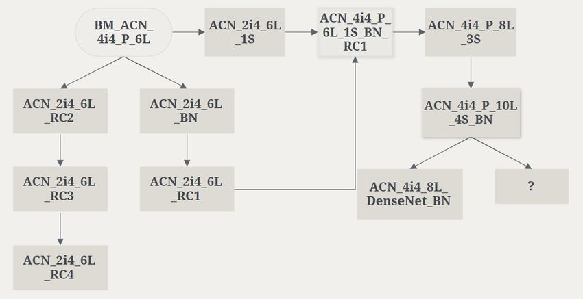
EPJ Web of Conferences 251, 04012 (2021)                          https://doi.org/10.1051/epjconf/202125104012
CHEP 2021

     Figure 2. Comparison between the performance of models reported in previous years (labeled ACAT-
     2019 and CtD-2020) and the new models described in detail in the text. An asymmetry parameter
     between the cost of overestimating contributions to the target histograms and underestimating them is
     varied to produce the families of points observed.

         Modified versions of our original CNN architecture [6] were studied to understand how
     performance depends on the number of model parameters, the number of network layers,
     the number of channels per layer, whether batch normalization is used, and the extent to
     which skip connections are used. We refer to these models as members of the AllCNN
     family. A one-dimensional version of the U-Net architecture [9], originally developed for
     two-dimensional biomedical images, was also tested using toy Monte Carlo and find that it
     (slightly) outperforms the best of our AllCNN models when both are trained with the same
     KDE.

     2 Performance Evolution
     Figure 2 shows how the performance of the KDE-to-hists algorithms have evolved over
     time. The solid blue circles show the performance of any early model described at ACAT-
     2019 [6]. The green squares and magenta diamonds show the performances described at
     Connecting-the-Dots in 2020 [7]. The efficiency is shown on the horizontal axis and the false
     positive rate per event is shown on the vertical axis. Both quantities are evaluated from a
     matching procedure done by a heuristic algorithm, based on the PV positions along the beam
     axis, z. A predicted PV is matched if the distance, ∆z, between it’s position, zpred , and the true
     PV position, ztrue , satisfies ∆z = |zpred − ztrue | ≤ 0.5mm. The false positive rate is obtained
     from ratio of remaining predicted PVs after the matching procedure over the total number of
     true PVs. An asymmetry parameter between the cost of overestimating contributions to the
     target histograms and underestimating them [6] is varied to produce the families of points
     observed. Those models were trained and tested using the original KDE and toy MC. The
     reported results, throughout this document, come from statistically independent validation
     samples. The model of the magenta diamonds was tested on full LHCb MC data in which the
     (original) KDE was derived from a full VELO tracking algorithm [8]. We observed slightly
     increased performance compared to toy MC (not shown). The model was then trained and
     tested using a full LHCb MC sample yielding significantly better results, shown as the red
     triangles in Fig.2. An algorithm that replaces the original KDE with two KDEs produces even
     better results, plotted as cyan-filled circles. The difference is most pronounced at efficiencies
     greater than ∼ 94%. The improved performance is primarily associated with correctly finding

                                                       3
EPJ Web of Conferences 251, 04012 (2021) https://doi.org/10.1051/epjconf/202125104012
CHEP 2021
true lower multiplicity PVs. Training the same model as that used to produce the red triangles,
but using one of the new KDEs in place of the original KDE, leads to worse performance. The
algorithm using both of the new KDEs learns how to combine their information effectively.
The plot also shows results for a U-Net model [9] using the same toy MC as used to train the
“traditional” KDE-to-hists models. Its performance is better than that of the other models
trained and tested on the same data. Its architecture is discussed below.
3 Kernel Density Estimators
Kernel generation converts sparse three-dimensional data into a small number of feature-
rich one-dimensional data sets. Deep neural networks (DNNs) can transform these into
one-dimensional histograms from which PV candidates are easily extracted. Each of our
one-dimensional data sets consists of 4000 bins along the z-direction (beamline), each
100 µm wide, spanning the active area of the VELO around the interaction point, such that
z ∈ [−100, 300] mm. In the original KDE, each z bin of the histogram is filled by the maxi-
mum kernel value in x and y, where the kernel is defined by
G(IP(x, y)|z)2
K(x, y, z) = tracks − G(IP(x, y)|z) . (1)
tracks G(IP(x, y)|z) tracks
In Eqn. (1), G(IP(x, y)|z) is a Gaussian function, centered at x = y = 0 and evaluated at
the impact parameter IP(x, y): the distance of closest approach of a track projection to a
hypothesized vertex at position x, y for a given z. The width/covariance of G is given by the
IP(x, y) uncertainty/covariance matrix. Finding the maximum K(x, y, z) is a two step process.
Kernel values are first computed in a coarse 8 × 8 grid in x, y; the parameters of that search
are then taken as starting points for a MINUIT minimization process to find the maximum
kernel value for each bin of z. The values of x and y where the kernel is maximum are saved
as secondary feature sets xMax and yMax
Equation (1) is computed from the location, direction, and covariance matrix of input
tracks. This information can be provided by a standalone toy Monte Carlo proto-tracking [6]
or from a proposed LHCb Run 3 production Velo tracking [8]. While the former uses a
heuristic Gaussian width to estimate the IP(x, y) uncertainty, the latter uses the measured
covariance matrix of the track state closest to beamline to compute the IP(x, y) covariance.
To reduce the computational load, the KDE contributions are only calculated in regions near
points where two tracks pass within 100 µm of each other. This is completely safe in terms
of finding true PV positions, but leads to discontinuities in KDE values as a function of z.
A first attempt to design an algorithm to predict KDE distributions from track parameters
led to relatively poor performances. It was designed to treat each track’s contribution to the
KDE separately. Adding the explicit requirement that a track contribute to the KDE only
when near another track allowed to increase the algorithm performances. More specifically,
the original KDE was replaced by a new one, KDE-A, based on each track’s position of
closest approach (poca) to the beamline and the error ellipsoid defined by
A(∆x)2 + B(∆y)2 + C(∆z)2 + 2(D∆x∆y + E∆x∆z + F∆y∆z) = 1 (2)
where ∆x = x − xpoca , etc. At any point in space, a Gaussian probability associated with this
track’s poca-ellipsoid is calculated as
exp −0.5(A(∆x)2 + B(∆y)2 + C(∆z)2 + 2(D∆x∆y + E∆x∆z + F∆y∆z)
G(x, y, z) = (3)
(ellipsoid volume)3/2
4EPJ Web of Conferences 251, 04012 (2021) https://doi.org/10.1051/epjconf/202125104012
CHEP 2021
Figure 3. This diagram illustrates the deep neural network used to predict an event’s KDE-A from
its tracks’ poca-ellipsoids. Twelve fully connected layers (all but the last with 50 neurons) populate
four 4000-bin channels in the last of these layers, for each track. These contributions are summed and
processed by two convolutional layers that provide a mechanism for the tracks to interact. A final fully
connected layer was required for the learning to converge.
For each voxel, the KDE-A contribution is calculated as the sum of poca-ellipsoid probabil-
ities:
KA = G(xi , yi , zi ) . (4)
tracks
where i denotes the track index. For each bin of z, the largest value of KA observed in an
(x, y, z) voxel is projected out as the KDE-A value at that value of z. However, the per-
formance of the KDE-to-hists algorithm using KDE-A in place of the original KDE was
significantly worse. As the definition of the original kernel in Eqn. 1 combined linear and
quadratic terms in G(IP(x, y)|z), we defined KDE-B using a procedure parallel to that for
defining KDE-A but replacing the linear sum of probabilities in KA with
KB = G(xi , yi , zi )2 . (5)
tracks
Using both KDE-A and KDE-B as input features, in place of the original KDE, improved
the performance of the KDE-to-hists algorithm, as noted in the earlier discussion of Fig. 2
(see the red triangles and cyan-filled circles).
While solely predicting KDE-A distributions from tracks parameters with reasonably
good fidelity using a DNN is quite strait-forward, achieving satisfactory performance does
require a mechanism that encourages the predictions for each track to interact with the pre-
dictions for the other tracks. This was studied using toy MC rather than full LHCb MC as
the former data sets are larger than the latter. For these, the model architecture was not opti-
mized – the choices of the numbers of layers of each type, the number of channels per layer,
the kernel sizes in the convolutional layers, etc., were chosen almost arbitrarily. With these
caveats, the architecture is illustrated in Fig. 3. Originally, there were 12 fully connected
layers that predicted KDE-A contributions for each track separately and then summed them.
The performance of this model was mediocre (at best). To allow the tracks to interact, the
single 4000-bin channel in the 12th layer that was originally meant to be the KDE prediction
was replaced by four latent 4000-bin channels. These are used as input to two convolutional
layers (and one more fully connected layer) that produce a final 4000-bin prediction. This
more complicated model was trained starting with the weights and biases of the first 11 fully
connected layers fixed while those of the new layers were learned. Once the full model began
5EPJ Web of Conferences 251, 04012 (2021) https://doi.org/10.1051/epjconf/202125104012
CHEP 2021
0.6 Toy MC simulation True KDE Toy MC simulation True PV position
0.3
Arbitrary unit
Arbitrary unit
Pred. KDE − PV #tracks = 10 True KDE
0.4 Visible PVs − PV z = −0.158 mm Pred. KDE
0.2
SVs
0.2 0.1
-100 -50 0 50 100 150 200 250 300 -4 -2 0 2 4
z [mm] z [mm]
Figure 4. The plot on the left illustrates KDE-A (shown in blue), calculated as described in the text
following Eqn. 5, and the KDE predicted by the DNN model described in the subsequent paragraph
(shown in red) for a single event. Each of the 4000 bins in the histogram corresponds to a range in the
z-direction of 100 µm. The plot on the right shows a zoomed-in view of the 50 bins on either side of the
location of the second PV in that event, whose location is denoted by the dashed vertical line.
to display a semblance of performance, all the model parameters were floated and learned
over many epochs, using progressively larger training samples. Fig. 4 compares KDE-A
(the blue histogram) for the first event in the validation sample with the corresponding KDE
predicted by the model (the red histogram) after about 300 hours of training on an nVidia
RTX2080Ti using PyTorch. Qualitatively, the predicted KDE reproduces the macroscopic
features of KDE-A, as seen in the plots on the left. On a finer scale, there are differences,
as seen in the plot on the right. This shows 50 bins on either side of the location of the first
PV in the event. The predicted KDE peaks at the location of the PV, as does KDE-A, but
its height is lower and its width is greater. This is typical of the learned KDE, although there
is tremendous variation from the region about one true PV in an event to another and from
event to event. A mean-squared-error function comparing the predicted KDE histogram to
the KDE-A is used to train the model. But the real goal is using a well-trained tracks-to-
KDE model as a step towards defining a tracks-to-hist model that performs at least as well
as the best model in Fig. 2.
As a proof-of-principle, we first trained a KDE-to-hists model using KDE-A as the only
input feature set. The efficiency and false positive rate were 94.3% and 0.27 per event. We
then merged the tracks-to-KDE model described above with this KDE-to-hists model to
create a tracks-to-hists model. With the weights of the combined model set to be those of the
independent models, the efficiency and false positive rate were approximately 88% and 0.88
per event. We then allowed the combined model to learn improved weights for the tracks-
to-KDE layers while the weights for the KDE-to-hists layers were held constant and vice
versa. In these cases, the improvements were very slow, with the efficiencies increasing a
(small) fraction of a percent and the false positive rates improving by less than 0.02 over the
course of several days training on nVidia RTX 2080Ti GPUs. Allowing all weights and biases
in the combined model to float produced significantly improved performance. After several
days of training, the efficiency increased to 91.0% and the false positive rate dropped to 0.80
per event before improvement completely plateaued.
As noted above, the predicted KDEs tend to produce broader features in the vicinity of
true PVs, as seen in Fig. 4. When increasing the threshold used in the matching procedure
from 500 to 750 µm, we observed a slight rise in efficiency, to 93.7%, and a drop in false pos-
itive rate to 0.69 per event. Although these efficiencies (original and alternative definitions)
are not as high as that of the KDE-to-hists model, and the false positive rates are higher,
the fact that simultaneously learning the combined model parameters produces significantly
better results than simply connecting the two networks with their independently learned pa-
rameters suggests that it should be possible to create a highly performant tracks-to-hists
6EPJ Web of Conferences 251, 04012 (2021) https://doi.org/10.1051/epjconf/202125104012
CHEP 2021
Figure 5. This plot illustrates the improved Figure 6. This plot illustrates the performance
performance of several models when xMax and of several models built from a benchmark model
yMax are added as perturbative features, as dis- with variations described in the text. The labels
cussed in the text. For each model, the open for each model encode the nature of the varia-
markers show the efficiency versus false positive tions, as described in Table 1 in the appendix. The
rate as the cost function asymmetry parameter is number of parameters learned by each model is
varied, while filled markers show the performance shown in parentheses to the right of its label.
when the perturbative features are added. Details
on the model variations are given in the appendix.
model. It also suggests that improving the tracks-to-KDE model so that it produces more
narrow peaks around PV positions will be necessary to significantly improve the merged
model performance.
4 Alternative Model Architectures
The architectures of the models whose performance is discussed in Sec. 2 and illustrated in
Fig. 2 are similar, but vary as discussed at conferences last year [7] and above. We have
now investigated some of these variations, and others, more systematically. We have stud-
ied a qualitatively new architecture as well. We find that adding the secondary feature sets
xMax and yMax to the models “perturbatively” systematically improves performance. We
also find that models with more parameters generally out-perform similar models with fewer
parameters. From a computer science perspective, the best performance may be considered
optimal. However, when deploying software for use in a HEP experiment, use of memory
and processor time may be considered as well. For example, it may be appropriate to trade
off small gains in performance if doing so requires only half the computing resources.
The results of adding perturbative features to three baseline models is illustrated in Fig. 5.
Once a model has been fully trained using only the KDE feature set, its weights and biases are
fixed and a second network is trained using only the secondary features; the final prediction
is the product of the two networks’ outputs (or generated from a sum or concatenation of
their outputs). After the secondary network is trained in this way, all the weights and biases
of the combined model are trained simultaneously to produce the final model. We find that
initially separating the baseline training from the secondary feature training is necessary for
deep learning to start. In each case shown (and others not shown to avoid visual congestion),
adding xMax and yMax features to the model perturbatively increases the efficiency and
reduces the false positive rate.
The benchmark model used as the starting point for studies of alternative models has six
convolutional layers, very similar to the model with four convolutional layers illustrated in
7EPJ Web of Conferences 251, 04012 (2021) https://doi.org/10.1051/epjconf/202125104012
CHEP 2021
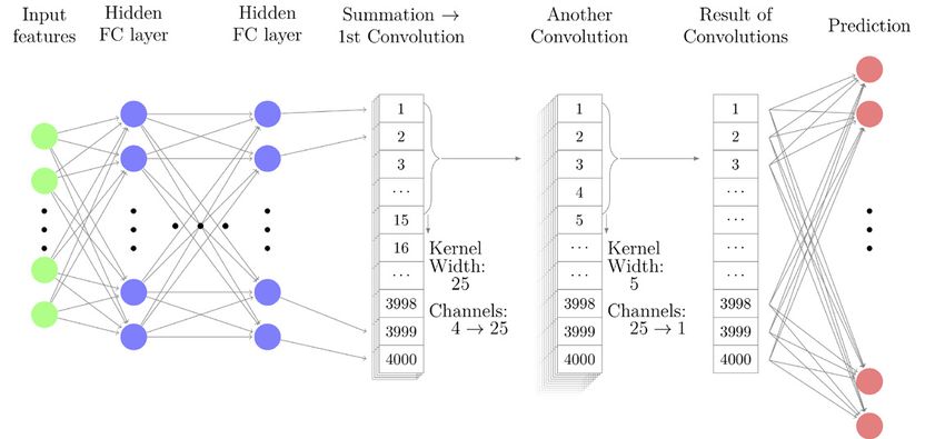
Figure 7. This is the architecture of a U-Net model modified for use in our one-dimensional KDE-
to-hists problem. The orange blocks are convolutional layers followed by ReLU activation functions,
the red blocks are down-sampling operations, and the blue blocks are up-sampling operations. The four
arrows that join down-sampling layers to up-sampling layers of the same dimensionality denote skip
connections.
Fig. 3 of Ref. [6]. In the results presented below, xMax and yMax have been added as per-
turbative features. The primary goal of these studies was to understand how the fidelity of a
model varies with the number of parameters and the use of skip connections, batch normal-
ization, etc. Table 1 in the appendix lists the types of variations that were considered. Results
from 5 of these models are shown in Fig. 6. In general, the larger the number of parameters,
the greater the fidelity of the model. That with the best performance is an adaptation of the
DenseNet architecture [10] which connects each layer to every other layer in a feed-forward
fashion, the ultimate limit adding skip connections. Note that these studies were done in par-
allel with others reported here. We have not yet incorporated what was learned here into, for
example, the best performing models of Fig. 2.
Inspired by its success solving other tasks that require shape-preservation between input
and output (object detection, semantic segmentation), we have modified the popular U-Net
architecture [9] for our one-dimensional problem. A diagram of the architecture is shown in
Fig. 7 – orange blocks are convolutional layers followed by ReLU activation functions, red
blocks are down-sampling operations (max pooling with kernel size and stride 2), and blue
blocks are up-sampling operations (transposed convolutions with kernel size and stride 2).
The arrows represent the flow of information throughout the network. It differs from a tradi-
tional autoencoder as some information bypasses successive layers and is added back in later
stages via a concatenation or addition operation (a skip connection). We investigated this ar-
chitecture for a number of reasons. Conceptually, it captures a receptive field that scales as 2n ,
where n is number of pooling operations. This can be compared to the AllCNN architectures
where the receptive field scales linearly with n. We hypothesize that the added ease in down-
sampling is important to achieve the granular resolution we want. In addition, we hypothesize
that the addition of skip connections up to the second-to-last layer in the network allows the
network to “remember” fine-grained detail about the input, and more effectively localize pri-
mary vertices. Experiments show that removing skip connections one-by-one consistently
degrades results by a minor amount. Including all four skip connections, the architecture
achieves an efficiency of 95% with a false-positive rate of 0.16 per event, slightly better than
the best AllCNN architecture using the same toy MC data and features. We anticipate that
this architecture will perform at least as well as the best AllCNN architecture when trained
using full LHCb MC plus KDE-A and KDE-B as input features.
8EPJ Web of Conferences 251, 04012 (2021) https://doi.org/10.1051/epjconf/202125104012
CHEP 2021
5 Summary and Conclusions
Since we presented results at Connecting-the-Dots 2020, we have tested AllCNN KDE-to-
hists models using full LHCb Monte Carlo rather than toy Monte Carlo and find they are (i)
more performant without re-training and (ii) even more performant with re-training. If we
replace the original KDE with a pair of KDEs, each built from individual track contributions
with no pairwise interactions used explicitly, the performance is better again. We have built
a deep learning tracks-to-KDE algorithm that reproduces the new KDE of Eqn. 5 with
sufficient fidelity that a merged tracks-to-hist algorithm achieves almost as high efficiency
as the underlying KDE-to-hist algorithm, albeit with worse resolution and a significantly
higher false positive rate. We conclude that the overall approach is sound, but we need to
construct and train a better tracks-to-KDE algorithm.
We have also performed systematic studies of alternative AllCNN models and a very
different model inspired by U-Net. The results of these studies indicate that the capacity of a
model to learn increases with the number of parameters and they suggest specific approaches
for improving the performance of the best KDE-to-hist model so far. The very similar
performance of the model inspired by U-Net and the best AllCNN model trained on the
same KDE invites the question of how two such different architectures have “learned” the
same “concepts” and whether such “understanding” can be generalized.
Two physics insights/hypotheses underly our current approach to developing hybrid deep
learning algorithms for identifying and locating primary vertices. First, tracks from pri-
mary vertices pass close enough to the beamline that each can be characterized by its poca-
ellipsoid. Second, the sparse three-dimensional information encoded in these ellipsoids can
be transformed to rich, one-dimensional KDEs that can, in turn, serve as input feature sets for
relatively simple deep neural networks. These can be trained on large samples of simulated
events (hundreds of thousands) to produce one-dimensional histograms that can be processed
by traditional, heuristic algorithms to extract information for the next stage of event recon-
struction and classification.
Our specific algorithms are being designed for use in LHCb with its Run 3 detector. As
the salient characteristics exist in the ATLAS and CMS experiments, as well, appropriately
modified versions might work for them. A heuristic ATLAS vertexing algorithm [11, 12], al-
ready uses some conceptually similar ideas, as does an algorithm [13] designed for the CMS
detector, upgraded for operation in the high luminosity LHC era. Developing and deploying
machine learning inference engines that are highly performant and satisfy computing sys-
tem constraints requires sustained effort. The results reported here should encourage work
focussed on using deep neural networks for identifying vertices in high energy physics ex-
periments.
6 Acknowledgments
The authors thank the LHCb computing and simulation teams for their support and for
producing the simulated LHCb samples used in this paper. The authors also thank the
full LHCb Real Time Analysis team, especially the developers of the VELO tracking al-
gorithm [8] used to generate the “full LHCb MC” results presented in Fig 2.
This work was supported, by the U.S. National Science Foundation under Cooperative
Agreement OAC-1836650 and awards PHY-1806260, OAC-1739772, and OAC-1740102.
9EPJ Web of Conferences 251, 04012 (2021) https://doi.org/10.1051/epjconf/202125104012
CHEP 2021
References
[1] R. Aaij et al. (LHCb), LHCb Trigger and Online Upgrade Technical Design Report
(2014), https://cds.cern.ch/record/1701361
[2] F. Reiss, Excerpts from the LHCb cookbook — RECEPTS for testing lepton universality
and reconstructing primary vertices (2020), presented 18 12 2020, https://cds.cern.
ch/record/2749592
[3] F. Reiss et al. (LHCb), Fast parallel Primary Vertex reconstruction for the LHCb Up-
grade (2020), talk presented at Connecting-the-Dots 2020, https://indico.cern.ch/
event/831165/timetable/?view=standard
[4] R. Aaij et al. (LHCb), JINST 14, P04013 (2019), arXiv:1812.10790
[5] R. Aaij et al. (LHCb), LHCb VELO Upgrade Technical Design Report (2013), https:
//cds.cern.ch/record/1624070
[6] R. Fang, H.F. Schreiner, M.D. Sokoloff, C. Weisser, M. Williams, J. Phys. Conf. Ser.
1525, 012079 (2020), arXiv:1906.08306
[7] S. Akar, T.J. Boettcher, S. Carl, H.F. Schreiner, M.D. Sokoloff, M. Stahl, C. Weisser,
M. Williams, An updated hybrid deep learning algorithm for identifying and locating
primary vertices (2020), arXiv:2007.01023
[8] A. Hennequin, B. Couturier, V. Gligorov, S. Ponce, R. Quagliani, L. Lacassagne, JINST
15, P06018 (2020), arXiv:1912.09901
[9] O. Ronneberger, P. Fischer, T. Brox, U-net: Convolutional networks for biomedical
image segmentation (2015), arXiv:1505.04597
[10] G. Huang, Z. Liu, L. Van Der Maaten, K.Q. Weinberger, Densely Connected Convolu-
tional Networks, in 2017 IEEE Conference on Computer Vision and Pattern Recognition
(CVPR) (2017), pp. 2261–2269, arXiv:1608.06993
[11] Development of ATLAS Primary Vertex Reconstruction for LHC Run 3 (2019), ATL-
PHYS-PUB-2019-015, https://cds.cern.ch/record/2670380
[12] I. Sanderswood (ATLAS), Development of ATLAS Primary Vertex Reconstruction for
LHC Run 3, in Connecting the Dots and Workshop on Intelligent Trackers (2019),
arXiv:1910.08405
[13] A. Bocci, M. Kortelainen, V. Innocente, F. Pantaleo, M. Rovere, Front. Big Data 3,
601728 (2020), arXiv:2008.13461
10EPJ Web of Conferences 251, 04012 (2021) https://doi.org/10.1051/epjconf/202125104012
CHEP 2021
Appendix: Models and Tags
The models discussed in the studies of systematic variations are derived from a benchmark
AllCNN model. The relationships between these models are shown in Fig. 8. As indicated in
Table 1, the numbers of layers, channels per layer, use of skip connections, batch normaliza-
tion, etc., could be varied. Not all combinations were studied, but the conclusion presented
in the body of the text – that increasing the numbers of parameters increases the capacity of
a network to learn well, almost independently of their origins – seems to be robust.
Figure 8. This figure shows how models studied relate to each other. The tags indicating the variations
in the architectures are described in Table 1.
These are the tags used to label each model name. The tags determine some of the key
features of the model at a high level.
Table 1. Neural network model tags for names
Tag V (Meaning)
#S number of skip connections, if any
#L number of layers
BN Batch Normalization
ACN AllCNN “family” of models
#i# step number out of total steps
RC# reduced channel size, followed by iteration number
IC# increased channel size, followed by iteration number
RK# reduced kernel size, followed by iteration number
IK# increased kernel size, followed by iteration number
C concatenation of perturbative and non-perturbative layers at end
BM benchmark; changes made to future models based on tagged reference model
The tag hierarchy is of the format:
BM-ACN-#i#-P-#L-#S-BN-RC-#-IC#-RK#-IK#-C
11You can also read