GANS CAN PLAY LOTTERY TICKETS TOO - OpenReview
←
→
Page content transcription
If your browser does not render page correctly, please read the page content below
Published as a conference paper at ICLR 2021

GAN S C AN P LAY L OTTERY T ICKETS T OO
 Xuxi Chen1* , Zhenyu Zhang1* , Yongduo Sui1 , Tianlong Chen2
 1
   University of Science and Technology of China, 2 University of Texas at Austin
 {chanyh,zzy19969,syd2019}@mail.ustc.edu.cn, tianlong.chen@utexas.edu

                                                A BSTRACT
             Deep generative adversarial networks (GANs) have gained growing popularity
             in numerous scenarios, while usually suffer from high parameter complexities for
             resource-constrained real-world applications. However, the compression of GANs
             has less been explored. A few works show that heuristically applying compression
             techniques normally leads to unsatisfactory results, due to the notorious training
             instability of GANs. In parallel, the lottery ticket hypothesis shows prevailing suc-
             cess on discriminative models, in locating sparse matching subnetworks capable of
             training in isolation to full model performance. In this work, we for the first time
             study the existence of such trainable matching subnetworks in deep GANs. For a
             range of GANs, we certainly find matching subnetworks at 67%-74% sparsity. We
             observe that with or without pruning discriminator has a minor effect on the exis-
             tence and quality of matching subnetworks, while the initialization weights used
             in the discriminator plays a significant role. We then show the powerful transfer-
             ability of these subnetworks to unseen tasks. Furthermore, extensive experimental
             results demonstrate that our found subnetworks substantially outperform previ-
             ous state-of-the-art GAN compression approaches in both image generation (e.g.
             SNGAN) and image-to-image translation GANs (e.g. CycleGAN). Codes avail-
             able at https://github.com/VITA-Group/GAN-LTH.

1       I NTRODUCTION
Generative adversarial networks (GANs) have been successfully applied to many fields like image
translation (Jing et al., 2019; Isola et al., 2017; Liu & Tuzel, 2016; Shrivastava et al., 2017; Zhu
et al., 2017) and image generation (Miyato et al., 2018; Radford et al., 2016; Gulrajani et al., 2017;
Arjovsky et al., 2017). However, they are often heavily parameterized and often require intensive
calculation at the training and inference phase. Network compressing techniques (LeCun et al.,
1990; Wang et al., 2019; 2020b; Li et al., 2020) can be of help at inference by reducing the number
of parameters or usage of memory; nonetheless, they can not save computational burden at no cost.
Although they strive to maintain the performance after compressing the model, a non-negligible
drop in generative capacity is usually observed. A question is raised:
Is there any way to compress a GAN model while preserving or even improving its performance?
The lottery ticket hypothesis (LTH) (Frankle & Carbin, 2019) provides positive answers with match-
ing subnetworks (Chen et al., 2020b). It states that there exist matching subnetworks in dense models
that can be trained to reach a comparable test accuracy to the full model within similar training iter-
ations. The hypothesis has successfully shown its success in various fields (Yu et al., 2020; Renda
et al., 2020; Chen et al., 2020b), and its property has been studied widely (Malach et al., 2020; Pen-
sia et al., 2020; Elesedy et al., 2020). However, it is never introduced to GANs, and therefore the
presence of matching subnetworks in generative adversarial networks still remains mysterious.
To address this gap in the literature, we investigate the lottery ticket hypothesis in GANs. One most
critical challenge of extending LTH in GANs emerges: how to deal with the discriminator while
compressing the generator, including (i) whether prunes the discriminator simultaneously and (ii)
what initialization should be adopted by discriminators during the re-training? Previous GAN com-
pression methods (Shu et al., 2019; Wang et al., 2019; Li et al., 2020; Wang et al., 2020b) prune the
generator model only since they aim at reducing parameters in the inference stage. The effect of
    ∗
        Equal Contribution.

                                                      1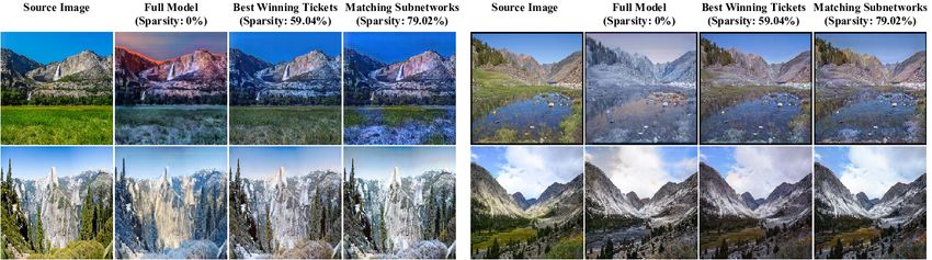
Published as a conference paper at ICLR 2021

pruning the discriminator has never been studied by these works, which is unnecessary for them
but possibly essential in finding matching subnetworks. It is because that finding matching sub-
networks involves re-training the whole GAN network, in which an imbalance in generative and
discriminative power could result in degraded training results. For the same reason, the disequilib-
rium between initialization used in generators and discriminators incurs severe training instability
and unsatisfactory results.
Another attractive property of LTH is the powerful transferability of located matching subnetworks.
Although it has been well studied in discriminative models (Mehta, 2019; Morcos et al., 2019; Chen
et al., 2020b), an in-depth understanding of transfer learning in GAN tickets is still missing. In
this work, we not only show whether the sparse matching subnetworks in GANs can transfer across
multiple datasets but also study what initialization benefits more to the transferability.
To convert parameter efficiency of LTH into the advantage of computational saving, we also utilize
channel pruning (He et al., 2017) to find the structural matching subnetworks of GANs, which
enjoys the bonus of accelerated training and inference. Our contributions can be summarized in the
following four aspects:

• Using unstructured magnitude pruning, we identify matching subnetworks at 74% sparsity in
  SNGAN (Miyato et al., 2018) and 67% in CycleGAN (Zhu et al., 2017). The matching subnet-
  works in GANs exist no matter whether pruning discriminators, while the initialization weights
  used in the discriminator are crucial.
• We show that the matching subnetworks found by iterative magnitude pruning outperform sub-
  networks extracted by randomly pruning and random initialization in terms of extreme sparsity
  and performance. To fully exploit the trained discriminator, we using the dense discriminator as
  a distillation source and further improve the quality of winning tickets.
• We demonstrate that the found subnetworks in GANs transfer well across diverse generative tasks.
• The matching subnetworks found by channel pruning surpass previous state-of-the-art GAN com-
  pression methods (i.e., GAN Slimming (Wang et al., 2020b)) in both efficiency and performance.

2   R ELATED W ORK
GAN Compression Generative adversarial networks (GANs) have succeeded in computer vision
fields, for example, image generation and translation. One significant drawback of the generative
models is the high computational cost of the models’ complex structure. A wide range of neural net-
work compression techniques has been applied to generative models to address this problem. There
are several categories of compression techniques, including pruning (removing some parameters),
quantization (reducing the bit width), and distillation. Shu et al. (2019) proposed a channel pruning
method for CycleGAN by using a co-evolution algorithm. Wang et al. (2019) proposed a quanti-
zation method for GANs based on the EM algorithm. Li et al. (2020) used a distillation method to
transfer knowledge of the dense to the compressed model. Recently Wang et al. (2020b) proposed
a GAN compression framework, GAN slimming, that integrated the above three mainstream com-
pression techniques into a unified form. Previous works on GAN pruning usually aim at finding a
sparse structure of the trained generator model for faster inference speed, while we are focusing on
finding trainable structures of GANs following the lottery ticket hypothesis. Moreover, in existing
GAN compression methods, only the generator is pruned, which could undermine the performance
of re-training since the left-out discriminator may have a stronger computational ability than the
pruned generator and therefore cause a degraded result due to the imparity of these two models.

The Lottery Ticket Hypothesis The lottery ticket hypothesis (LTH) (Frankle & Carbin, 2019)
claims the existence of sparse, separate trainable sub-networks in a dense network. These subnet-
works are capable of reaching comparable or even better performance than full dense model, which
has been evidenced in various fields, such as image classification (Frankle & Carbin, 2019; Liu et al.,
2019; Wang et al., 2020a; Evci et al., 2019; Frankle et al., 2020; Savarese et al., 2020; Yin et al.,
2020; You et al., 2020; Ma et al., 2021; Chen et al., 2020a), natural language processing (Gale et al.,
2019; Chen et al., 2020b), reinforcement learning (Yu et al., 2020), lifelong learning (Chen et al.,
2021b), graph neural networks (Chen et al., 2021a), and adversarial robustness (Cosentino et al.,
2019). Most works of LTH use unstructured weight magnitude pruning (Han et al., 2016; Frankle &

                                                  2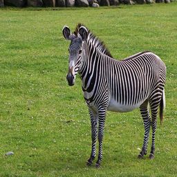
Published as a conference paper at ICLR 2021

Carbin, 2019) to find the matching subnetworks, and the channel pruning is also adopted in a recent
work (You et al., 2020). In order to scale up LTH to larger networks and datasets, the “late rewind-
ing” technique is proposed by Frankle et al. (2019); Renda et al. (2020). Mehta (2019); Morcos
et al. (2019); Desai et al. (2019) are the pioneers to study the transferability of found subnetworks.
However, all previous works focus on discriminative models. In this paper, we extend LTH to GANs
and reveal unique findings of GAN tickets.

3   P RELIMINARIES
In this section, we describe our pruning algorithms and list related experimental settings.

Backbone Networks We use two GANs in our experiments in Section 4: SNGAN (Miyato et al.,
2018) and CycleGAN (Zhu et al., 2017)). SNGAN with ResNet (He et al., 2016) is one of the most
popular noise-to-image GAN network and has strong performance on several datasets like CIFAR-
10. CycleGAN is a popular and well-studied image-to-image GAN network that also performs well
on several benchmarks. For SNGAN, let g(z; θg ) be the output of the generator network G with
parameters θg and a latent variable z ∈ Rkzk0 and d(x; θd ) be the output of the discriminator
network D with parameters θd and input example x. For CycleGAN which is composed of two
generator-discriminator pairs, we use g(x; θg ) and θg again to represent the output and the weights
of the two generators where x = (x1 , x2 ) indicates a pair of input examples. The same modification
can be done for the two discriminators in CycleGAN.

Datasets For image-to-image experiments, we use a widely-used benchmark horse2zebra (Zhu
et al., 2017) for model training. As for noise-to-image experiments, we use CIFAR-10 (Krizhevsky
et al., 2009) as the benchmark. For the transfer study, the experiments are conducted on CIFAR-10
and STL-10 (Coates et al., 2011). For better transferring, we resize the image in STL-10 to 32 × 32.

Subnetworks For a network f (·; θ) parameterized by θ, a subnetwork is defined as f (·;m θ),
where m ∈ {0, 1}kθk0 is a pruning mask for θ ∈ Rkθk0 and is the element-wise product. For
GANs, two separate masks, md and mg , are needed for both the generator and the discriminator.
Consequently, a subnetwork of GANs is consistent of: a sparse generator g(·; mg θg ) and a sparse
discriminator d(·; md θd ).
Let θ0 be the initialization weights of model f and θt be the weights at training step t. Follow-
ing Frankle et al. (2019), we define a matching network as a subnetwork f (·; m θ), where θ is
initialized with θt , that can reach the comparable performance to the full network within a similar
training iterations when trained in isolation; a winning ticket is defined as a matching subnetwork
where t = 0, i.e. θ initialized with θ0 .

Finding subnetworks Finding GAN subnetworks is to find two masks mg and md for the gen-
erator and the discriminator. We use both an unstructured magnitude method, i.e. the iterative
magnitude pruning (IMP), and a structured pruning method, i.e. the channel pruning (He et al.,
2017), to generate the masks.
For unstructured pruning, we follow the following steps. After we finish training the full GAN
model for N iterations, we prune the weights with the lowest magnitude globally (Han et al., 2016)
to obtain masks m = (mg , md ), where the position of a remaining weight in m is marked as one,
and the position of a pruned weight is marked as zero. The weights of the sparse generator and the
sparse discriminator are then reset to the initial weights of the full network. Previous works have
shown that the iterative magnitude pruning (IMP) method is better than the one-shot pruning method.
So rather than pruning the network only once to reach the desired sparsity, we prune a certain amount
of non-zero parameters and re-train the network several times to meet the requirement. Details of
this algorithm are in Appendix A1.1, Algorithm 1.
As for channel pruning, the first step is to train the full model as well. Besides using a normal loss
function LGAN , we follow Liu et al. (2017) to apply a `1 -norm on the trainable scale parameters
γ in the normalization layers to encourage channel-level sparsity: Lcp = ||γ||1 . To prevent the
compressed network behave severely differently with the original large network, we introduce a
distillation loss as Wang et al. (2020b) did: Ldist = Ez [dist(g(z; θg ), g(z; mg θg ))]. We train the

                                                  3
Published as a conference paper at ICLR 2021

GAN network with these two additional losses for N1 epochs and get the sparse networks g(·; mg
θg ) and d(·; md θg ). Details of this algorithm are in Appendix A1.1, Algorithm 2.

Evaluation of subnetworks After obtaining the subnetworks g(·; θg mg ) and d(·; θd md ),
we test whether the subnetworks are matching or not. We reset the weights to a specific step i,
and train the subnetworks for N iterations and evaluate them using two specific metrics, Inception
Score (Salimans et al., 2016) and Fréchet Inception Distance (Heusel et al., 2017).

Other Pruning Methods We compare the size and the performance of subnetworks found by IMP
with subnetworks found by other techniques that aim at compressing the network after training to
reduce computational costs at inference. We use a benchmark pruning approach named Standard
Pruning (Chen et al., 2020b; Han et al., 2016), which iteratively prune the 20% of lowest magnitude
weights, and train the network for another N iterations without any rewinding, and repeat until we
have reached the target sparsity.
In order to verify that the statement of iterative magnitude pruning is better than one-shot pruning,
we compare IMPG and IMPGD with their one-shot counterparts. Additionally, we compare IMP
with some randomly pruning techniques to prove the effectiveness of IMP. They are: 1) Randomly
Pruning: Randomly generate a sparsity mask m0 . 2) Random Tickets: Rewinding the weights to
another initialization θ00 .

4       T HE E XISTENCE OF W INNING T ICKETS IN GAN

In this section, we will validate the existence of winning tickets in GANs with initialization θ0 :=
(θg0 , θd0 ). Specifically, we will empirically prove several important properties of the tickets by
authenticating the following four claims:
Claim 1: Iterative Magnitude Pruning (IMP) finds winning tickets in GANs, g(·; mg            θg0 ) and
d(·; md θd0 ). Channel pruning is also able to find winning tickets as well.
Claim 2: Whether pruning the discriminator D does not change the existence of winning tickets. It
is the initialization used in D that matters. Moreover, pruning the discriminator has a slight boost of
matching networks in terms of extreme sparsity and performance.
Claim 3: IMP finds winning tickets at sparsity where some other pruning methods (randomly prun-
ing, one-shot magnitude pruning, and random tickets) are not matching.
Claim 4: The late rewinding technique (Frankle et al., 2019) helps. Matching subnetworks that are
initialized to θi , i.e., i steps from θ0 , can outperform those initialized to θ0 . Moreover, matching
subnetworks that are late rewound can be trained to match the performance of standard pruning.

Claim 1: Are there winning tickets in GANs? To answer this question, we first conduct ex-
periments on SNGAN by pruning the generator only in the following steps: 1) Run IMP to get
sequential sparsity masks (mdi , mgi ) of sparsity si % remaining weights; 2) Apply the masks to
the GAN and reset the weights of the subnetworks to the same random initialization θ0 ; 3) Train
models to evaluate whether they are winning tickets. 1 We set si % = (1 − 0.8i ) × 100%, which
we use for all the experiments that involve iteratively pruning hereinafter. The number of training
epochs for subnetworks is identical to that of training the full models.
Figure 1 verifies the existence of winning tickets in SNGAN and CycleGAN. We are able to find
winning tickets by iterative pruning the generators at the highest sparsity, around 74% in SNGAN,
and around 67% in CycleGAN, where the FID scores of these subnetworks successfully match the
FID scores of the full network respectively. The confidence interval also suggests that the winning
tickets at some sparsities are statistically significantly better than the full model.
To show that channel pruning can find winning tickets as well, we extract several subnetworks from
the trained full SNGAN and CycleGAN by varying ρ in Algorithm 2. We define the channel-pruned
model’s sparsity as the ratio of MFLOPs between the sparse model and the full model.
    1
        The detailed description of algorithms are listed in Appendix A1.1.

                                                         4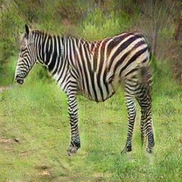
Published as a conference paper at ICLR 2021
150
20
125
FID 18
FID
100
CIFAR−10 horse2zebra
16
zebra2horse
75
14 50
.0
.0
.0
.2
.0
.8
.2
.0
13.8
10.4
.7
.0
.0
.0
.2
.0
.8
.2
.0
13.8
10.4
.7
0
80
64
51
41
32
26
21
16
0
80
64
51
41
32
26
21
16
10
10
Remaining Weights (%) Remaining Weights (%)
Figure 1: The Fréchet Inception Distance (FID) curve of subnetworks of SNGAN (left) and CycleGAN (right)
generated by iterative magnitude pruning (IMP) on CIFAR-10 and horse2zebra. The dashed line indicates the
FID score of the full model on CIFAR-10 and horse2zebra. The 95% confidence interval of 5 runs is reported.
We can confirm that winning tickets can also be found by channel pruning (CP). CP is able to find
winning tickets in SNGAN at sparsity around 34%. We will analyze it more carefully in Section 7.
Full Model (Sparsity: 0%) Best Winning Tickets (Sparsity: 48.80%) Matching Subnetworks (Sparsity: 73.79%)
Interpolation Generation
Figure 2: Visualization by sampling and interpolation of SNGAN Winning Tickets found by IMP. Sparsity of
best winning tickets : 48.80%. Extreme sparsity of matching subnetworks: 73.79%.
Source Image Full Model Best Winning Tickets Matching Subnetworks Source Image Full Model Best Winning Tickets Matching Subnetworks
(Sparsity: 0%) (Sparsity: 59.04%) (Sparsity: 67.24%) (Sparsity: 0%) (Sparsity: 59.04%) (Sparsity: 67.24%)
Figure 3: Visualization of CycleGAN Winning Tickets found by IMP. Sparsity of best winning tickets :
59.04%. Extreme sparsity of matching subnetworks: 67.24%. Left: visualization results on horse2zebra.
Right: visualization results on zebra2horse.
Claim 2: Does the treatment of the discriminator affect the existence of winning tickets? Pre-
vious works of GAN pruning did not analyze the effect of pruning the discriminator. To study the
effect, we compare two different iterative pruning settings: 1) Prune the generator only (IMPG ) and
2) Prune both the generator and the discriminator iteratively (IMPGD ). Both the generator and the
discriminator are reset to the same random initialization θ0 after the masks are obtained.
The FID scores of the two experiments are shown in Figure 4. The graph suggests that the two
settings share similar patterns: the minimal FID of IMPG is 14.19, and the minimal FID of IMPGD
is 14.59. The difference between these two best FID is only 0.4, showing a slight difference in
generative power. The FID curve of IMPG lies below that of IMPGD at low sparsity but lies above
at high sparsity, indicating that pruning the discriminator produces slightly better performance when
the percent of remaining weights is small. The extreme sparsity where IMPGD can match the
performance of the full model is 73.8%. In contrast, IMPG can only match no sparser than 67.2%,
demonstrating that pruning the discriminator can also push the frontier of extreme sparsity where
the pruned models are still able to match.
In addition, we study the effects of different initialization for the sparse discriminator. We compare
different weights loading methods when applying the iterative magnitude pruning process: 1) Reset
the weights of generator to θg0 and reset the weights of discriminator to θd0 , which is identical
to IMPG ; 2) Reset the weights of generator to θg0 and fine-tune the discriminator, which we will
call IMPF G . Figure 4 shows that resetting both the weights to θ0 produces a much better result than
5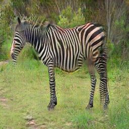
Published as a conference paper at ICLR 2021
only resetting the generator. The discriminator D without resetting its weights is too strong for the
generator G with initial weights θg0 that will lead to degraded performance. In summary, different
initialization of the discriminator will significantly influence the existence and quality of winning
tickets in GAN models.
75
18
IMPG
IMPGD
FID
FID
50
16 IMPG
IMPFG
25
14
.0
.0
.0
.2
.0
.8
.2
.0
13.8
10.4
.7
.0
.0
.0
.2
.0
.8
.2
.0
13.8
10.4
.7
0
80
64
51
41
32
26
21
16
0
80
64
51
41
32
26
21
16
10
10
Remaining Weights (%) Remaining Weights (%)
Figure 4: The FID score of Left: The FID score of best subnetworks generated by two different pruning
settings: IMPG and IMPGD . Right: The FID score of best subnetworks generated by two different pruning
settings: IMPG and IMPF G . IMPG : iteratively prune and reset the generator. IMPGD : iteratively prune and
reset the generator and the discriminator. IMPFG : iteratively prune and reset the generator, and iteratively prune
but not reset the discriminator.
A follow-up question arises from the previous observations: is there any way to use the weights of
the dense discriminator, as the direct usage of the dense weights yields inferior results? One possible
way is to use it as a “teacher” and transfer the knowledge to pruned discriminator using a consistency
loss. Formally speaking, an additional regularization term is used when training the whole network:
LKD (x; θd , md ) = Ex [KLDiv (d(x; md θd ), d(x; θd1 ))]
where KLDiv denotes the KL-Divergence. We name the iterative pruning method with this additional
regularization IMPKD
GD .
Figure 5 shows the result of pruning method IMPG
IMPKD GD compared to the previous two prun-
18 IMPGD
IMPKD
GD
ing methods we proposed, IMPG and IMPGD .
FID
IMPKD GD is capable of finding winning tickets
16
at sparsity around 70%, outperforming IMPG ,
and showing comparable results to IMPGD re- 14
garding the extreme sparsity. The FID curve of
.0
0
0
2
0
8
.2
.0
13.8
10.4
.7
.
.
.
.
.
0
80
64
51
41
32
26
21
16
setting IMPKD
10
GD is further mostly located below Remaining Weights (%)
the curve of IMPGD , demonstrating a stronger Figure 5: The FID curve of best subnetworks gen-
generative ability than IMPGD . It suggests erated by three different pruning methods: IMPG ,
transferring knowledge from the full discrimi- IMPGD and IMPKD KD
GD . IMPGD : iteratively prune and
nator benefits to find the winning tickets. reset both the generator and the discriminator, and train
them with the KD regularization.
Claim 3: Can IMP find matching subnetworks sparser than other pruning methods? Pre-
vious works claim that both a specific sparsity mask and a specific initialization are necessary for
finding winning tickets (Frankle & Carbin, 2019), and iterative magnitude pruning is better than
one-shot pruning. To extend such a statement in the context of GANs, we compare IMP with several
other benchmarks, randomly pruning (RP), one-shot magnitude pruning (OMP), and random tickets
(RT), to see if IMP can find matching networks at higher sparsity.
Method FIDBest (Sparsity) FIDExtreme (Sparsity)
IMPG
20 IMPGD No Pruning 15.69 (0.0%) -
OMPG
OMPGD IMPG 14.19 (20.0%) 15.58 (67.2%)
FID
18
IMPGD 14.59 (59.0%) 15.53 (73.8%)
OMPG 14.36 (36.0%) 15.33 (59.0%)
16
OMPGD 14.52 (20.0%) 15.69 (48.8%)
14 Table 1: The extreme sparsity of the matching net-
.0
.0
.0
.2
.0
.8
.2
.0
13.8
10.4
.7
0
80
64
51
41
32
26
21
16
works and the FID score of best subnetworks, found
10
Remaining Weights (%)
by iterative pruning and one-shot pruning. OMPG :
Figure 6: FID curves: OMPG , IMPG , OMPGD one-shot prune the generator. OMPGP : one-shot
and IMPGD . OMPG : one-shot prune the generator.
prune generator/discriminator.
OMPGP : one-shot prune generator/discriminator.
6
Published as a conference paper at ICLR 2021

Figure 6 and Table 1 show that iterative magnitude pruning outperforms one-shot magnitude pruning
no matter pruning the discriminator or not. IMP finds winning tickets at higher sparsity (67.23% and
73.79%, respectively) than one-shot pruning (59.00% and 48.80%, respectively). The minimal FID
score of subnetworks found by IMP is smaller than that of subnetworks found by OMP as well. This
observation defends the statement that pruning iteratively is superior compared to one-shot pruning.
We also list the minimal FID scores and extreme sparsity of matching networks for other pruning
methods in Figure 7 and Table 2. It can be seen that IMP finds winning tickets at sparsity where
some other pruning methods, randomly pruning and random initialization, cannot match. Since
IMPG shows the best overall result, we authenticate the previous statement that both the specific
sparsity mask and the specific initialization are essential for finding winning tickets.

                                                                           Method        FIDBest (Sparsity)   FIDExtreme (Sparsity)
                IMPG                                                      No Pruning       15.69 (0.0%)
      25          RT
                  RP                                                        IMPG           14.19 (20.0%)         15.58 (67.2%)
                                                                        Random Pruning     14.57 (20.0%)         15.60 (36.0%)
FID

      20                                                                Random Tickets     14.28 (36.0%)         15.33 (59.0%)

      15
                                                                       Table 2: The FID score of best subnetworks and the
                                                                       extreme sparsity of matching networks found by Ran-
           0

                       .0

                               .0

                                       .2

                                             .0

                                                     .8

                                                              .2
                                                              .0
                                                           13.8
                                                           10.4
                                                              .7
           0.

                   80

                              64

                                      51

                                            41

                                                    32

                                                          26
                                                           21
                                                           16
       10

                            Remaining Weights (%)                      dom Pruning, Random Rickets, and iterative magni-
Figure 7: The FID curve of best subnetworks gener-                     tude pruning.
ated by three different pruning settings: IMPG , RP,
and RT. RP: iteratively randomly prune the genera-
tor. RT: iteratively prune the generator but reset the
weights randomly.

Claim 4: Does rewinding improve performance? In previous paragraphs, we show that we are
able to find winning tickets in both SNGAN and CycleGAN. However, these subnetworks cannot
match the performance of the original network at extremely high sparsity, while the subnetworks
found by standard pruning can (Table 3). To find matching subnetworks at such high sparsity, we
adopt the rewinding paradigm: after the masks are obtained, the weights of the model are rewound to
θi , the weights after i steps of training, rather than reset to the same random initialization θ0 . It was
pointed out by Renda et al. (2020) that subnetworks found by IMP and rewound early in training can
be trained to achieve the same accuracy at the same sparsity as subnetworks found by the standard
pruning, providing a possibility that rewinding can also help GAN subnetworks.
We choose different rewinding settings: 5%, Table 3: Rewinding results. SExtreme : Extreme spar-
10%, and 20% of the whole training epochs. sity where matching subnetworks exist. FIDBest : The
The results are shown in Table 3. We observe minimal FID score of all subnetworks. FID89% : The
that rewinding can significantly increase the ex- FID score of subnetworks at 89% sparsity.
treme sparsity of matching networks. Rewind-        Setting of rewinding SExtreme FIDBest FID89%
ing to even only 5% of the training process         Rewind 0%            67.23%     14.20   19.60
can raise the extreme sparsity from 67.23% to       Rewind 5%            86.26%     13.96   15.82
86.26%, and rewinding to 20% can match the          Rewind 10%           86.26%     14.43   15.63
performance of standard pruning. We also com-       Rewind 20%           89.26%     14.82   15.29
pare the FID score of subnetworks found at          Standard Pruning     89.26%     14.18   15.22
89% sparsity. Rewind to 20% of the training
process can match the performance of standard pruning at 89% sparsity, and other late rewinding
settings can match the performance of the full model. This suggests that late rewinding techniques
can greatly contribute to matching subnetworks with higher sparsity.
Summary Extensive experiments are conducted to examine the existence of matching subnet-
works in generative adversarial models. We confirmed that there were matching subnetworks at
high sparsities, and both the sparsity mask and the initialization matter for finding winning tickets.
We also studied the effect of pruning the discriminator and demonstrate that pruning the discrimi-
nator can slightly boost the performance regarding the extreme sparsity and the minimal FID. We
proposed a method to utilize the weights of the dense discriminator model to boost the performance
further. We also compare IMP with different pruning methods, showing that IMP is superior to ran-
dom tickets and random pruning. In addition, late rewinding can match the performance of standard
pruning, which again shows consistency with previous works.

                                                                   7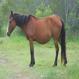
Published as a conference paper at ICLR 2021

5     T HE TRANSFER LEARNING OF GAN MATCHING NETWORKS
In the previous section, we confirm the presence of winning tickets in GANs. In this section, we will
study the transferability of winning tickets. Existing works (Mehta, 2019) show that the matching
networks in discriminative models can transfer across tasks. Here we evaluate this claim in GANs.
To investigate the transferability, we propose three transfer experiments from CIFAR-10 to STL-10
on SNGAN. We first identify matching subnetworks g(·, mg θ) and d(·, md θ) on CIFAR-
10, and then train and evaluate the subnetworks on STL-10. To assess whether the same random
initialization θ0 is needed for transferring, we test three different weights loading method: 1) reset
the weights to θ0 ; 2) reset the weights to another initialization θ00 ; 3) rewind the weights to θN . We
train the network on STL-10 using the same hyper-parameters as on CIFAR-10. It is noteworthy
that the hyper-parameters setting might not be optimal for the target task, yet it is fair to compare
different transferring settings.
Table 4: Results of late rewinding experiments. θ0 : train the target model from the same random initialization
as the source model; θr : train from random initialization; θBest : train from the weights of trained source
model. Baseline: full model trained on STL-10.
    Model     Baseline     IMPG (S = 67.23%)           IMPGD (S = 73.79%)          IMPKD
                                                                                      GD (S = 73.79%)
    Metrics   FIDBest      FIDBest     Matching?       FIDBest      Matching?      FIDBest       Matching?
      θ0                    116.7           X             121.8          ×           120.1           ×
      θr       115.3        119.2           ×             113.1          X           115.5           X
    θBest                   204.7           ×             163.0          ×           179.1           ×

The FID score of different settings is shown in Table 4. Subnetworks initialized by θ0 and using
masks generated by IMPG can be trained to achieve comparable results to the baseline model. Sur-
prisingly, random re-initialization θ00 shows better transferability than using the same initialization
θ0 in our transfer settings and outperforms the full model trained on STL-10, indicating that the
combination of θ0 and the mask generated by IMPGD is more focused on the source dataset and
consequently has lower transferability.

Summary In this section, we tested the transferability of IMP subnetworks. Transferring from θ0
and θr both produce matching results on the target dataset, STL-10. θ0 works better with masks
generated by IMPG while the masks generated by IMPGD prefer a different initialization θr . Given
that IMPGD performs better on CIFAR-10, it is reasonable that the same initialization θ0 has lower
transferability when using masks from IMPGD .

6     E XPERIMENTS ON OTHER GAN MODELS AND OTHER DATASETS

We conducted experiments on DCGAN (Radford et al., 2016), WGAN-GP (Gulrajani et al., 2017),
ACGAN (Odena et al., 2017), GGAN (Lim & Ye, 2017), DiffAugGAN (Zhao et al., 2020a), Pro-
jGAN (Miyato & Koyama, 2018), SAGAN (Zhang et al., 2019), as well as a NAS-based GAN,
AutoGAN (Gong et al., 2019). We use CIFAR-10 and Tiny ImageNet (Wu et al., 2017) as our
benchmark datasets.
Table 5 and 6 consistently verify that the existence of winning tickets in diverse GAN architectures in
spite of the different extreme sparsities, showing that the lottery ticket hypothesis can be generalized
to various GAN models.

7     E FFICIENCY OF GAN W INNING T ICKETS

Unlike the unstructured magnitude pruning method, channel pruning can reduce the number of pa-
rameters in GANs. Therefore, winning tickets found by channel pruning are more efficient than the
original model regarding computational cost. To fully exploit the advantage of subnetworks founded
by structural pruning, we further compare our prune-and-train pipeline with a state-of-the-art GAN
compression framework (Wang et al., 2020b). The pipeline is described as follows: after extracting
the sparse structure generated by channel pruning, we reset the model weights to the same random
initialization θ0 and then train for the same number of epochs as the dense model used.

                                                      8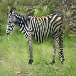
Published as a conference paper at ICLR 2021

Table 5: Results on other GAN models on CIFAR-10. FIDFull : FID score of the full model. FIDBest :
The minimal FID score of all subnetworks. FIDExtreme : The FID score of matching networks at
extreme sparsity level. AutoGAN-A/B/C are three representative GAN architectures represented in
the official repository (https://github.com/VITA-Group/AutoGAN)
                  Model                  Benchmark      FIDFull (Sparsity)                FIDBest (Sparsity)          SExtreme (Sparsity)
       DCGAN (Radford et al., 2016)       CIFAR-10         57.39 (0%)                          49.31 (20.0%)                54.48 (67.2%)
     WGAN-GP (Gulrajani et al., 2017)     CIFAR-10         19.23 (0%)                          16.77 (36.0%)                17.28 (73.8%)
       ACGAN (Odena et al., 2017)         CIFAR-10         39.26 (0%)                          31.45 (36.0%)                38.95 (79.0%)
         GGAN (Lim & Ye, 2017)            CIFAR-10         38.50 (0%)                          33.42 (20.0%)                36.67 (48.8%)
    ProjGAN (Miyato & Koyama, 2018)       CIFAR-10         31.47 (0%)                          28.19 (20.0%)                31.31 (67.2%)
        SAGAN (Zhang et al., 2019)        CIFAR-10         14.73 (0%)                          13.57 (20.0%)                14.68 (48.8%)
     AutoGAN(A) (Gong et al., 2019)       CIFAR-10         14.38 (0%)                          14.04 (36.0%)                14.04 (36.0%)
     AutoGAN(B) (Gong et al., 2019)       CIFAR-10         14.62 (0%)                          13.16 (20.0%)                14.20 (36.0%)
     AutoGAN(C) (Gong et al., 2019)       CIFAR-10         13.61 (0%)                          13.41 (48.8%)                13.41 (48.8%)
     DiffAugGAN (Zhao et al., 2020b)      CIFAR-10          8.23 (0%)                          8.05 (48.8%)                 8.05 (48.8%)

Table 6: Results on other GAN models on Tiny ImageNet. FIDFull : FID score of the full model.
FIDBest : The minimal FID score of all subnetworks. FIDExtreme : The FID score of matching
networks at extreme sparsity level.
                 Model                   Benchmark       FIDFull (Sparsity)               FIDBest (Sparsity)              SExtreme (Sparsity)
     DCGAN (Radford et al., 2016)       Tiny ImageNet      121.35 (0%)                         78.51 (36.0%)               114.00 (67.2%)
    WGAN-GP (Gulrajani et al., 2017)    Tiny ImageNet      211.77 (0%)                         194.72 (48.8%)              200.22 (67.2%)

We can see from Figure 8 that subnetworks are founded by the channel pruning method at about 67%
sparsity, which provides a new path for winning tickets other than magnitude pruning. The matching
networks at 67.7% outperform GS-32 regarding Inception Score by 0.25; the subnetworks at about
29% sparsity can outperform GS-32 by 0.20, setting up a new benchmark for GAN compressions.

8      C ONCLUSION

In this paper, the lottery ticket hypothesis has
been extended to GANs. We successfully iden-                                Full Model
tify winning tickets in GANs, which are sep-                    8.25
arately trainable to match the full dense GAN
performance. Pruning the discriminator, which                   8.00
                                                           IS

                                                                               CIFAR−10                GS−32
is rarely studied before, had only slight effects
on the ticket finding process, while the initial-               7.75
ization used in the discriminator is essential.
                                                                                                                                       GS−32
We also demonstrate that the winning tickets
                                                                            0
                                                                           .1

                                                                                     .8

                                                                                           .9

                                                                                                  .7

                                                                                                        .7

                                                                                                                .4

                                                                                                                      .2

                                                                                                                                            .5
                                                                         0.
                                                                        96

                                                                                    88

                                                                                          82

                                                                                                 76

                                                                                                       67

                                                                                                               59

                                                                                                                     54

                                                                                                                                         28

found can transfer across diverse tasks. More-
                                                                       10

                                                                                                  Remaining Weights (%)
over, we provide a new way of finding winning              Figure 8: Relationship between the best IS score of
tickets that alter the structure of models. Chan-          SNGAN subnetworks generated by channel pruning
nel pruning is able to extract matching subnet-            and the percent of remaining weights. GS-32: GAN
works from a dense model that can outperform               Slimming without quantization (Wang et al., 2020b).
the current state-of-the-art GAN compression               Full Model: Full model trained on CIFAR-10.
after resetting the weights and re-training.

ACKNOWLEDGEMENT

Zhenyu Zhang is supported by the National Natural Science Foundation of China under grand
No.U19B2044.

                                                          9
Published as a conference paper at ICLR 2021

R EFERENCES
Martin Arjovsky, Soumith Chintala, and Léon Bottou. Wasserstein generative adversarial networks.
 In Proceedings of the 34th International Conference on Machine Learning, 2017.
Tianlong Chen, Jonathan Frankle, Shiyu Chang, Sijia Liu, Yang Zhang, Michael Carbin, and
  Zhangyang Wang. The lottery tickets hypothesis for supervised and self-supervised pre-training
  in computer vision models. arXiv, abs/2012.06908, 2020a.
Tianlong Chen, Jonathan Frankle, Shiyu Chang, Sijia Liu, Yang Zhang, Zhangyang Wang,
  and Michael Carbin. The lottery ticket hypothesis for pre-trained bert networks. arXiv,
  abs/2007.12223, 2020b.
Tianlong Chen, Yongduo Sui, Xuxi Chen, Aston Zhang, and Zhangyang Wang. A unified lottery
  ticket hypothesis for graph neural networks, 2021a.
Tianlong Chen, Zhenyu Zhang, Sijia Liu, Shiyu Chang, and Zhangyang Wang. Long live the lottery:
  The existence of winning tickets in lifelong learning. In International Conference on Learning
  Representations, 2021b.
Adam Coates, Andrew Y. Ng, and Honglak Lee. An analysis of single-layer networks in unsuper-
  vised feature learning. In Proceedings of the 14th International Conference on Artificial Intelli-
  gence and Statistics, 2011.
Justin Cosentino, Federico Zaiter, Dan Pei, and Jun Zhu. The search for sparse, robust neural
  networks. arXiv, abs/1912.02386, 2019.
Shrey Desai, Hongyuan Zhan, and Ahmed Aly. Evaluating lottery tickets under distributional shifts.
  In Proceedings of the 2nd Workshop on Deep Learning Approaches for Low-Resource NLP, 2019.
Bryn Elesedy, Varun Kanade, and Y. Teh. Lottery tickets in linear models: An analysis of iterative
  magnitude pruning. arXiv, abs/2007.08243, 2020.
Utku Evci, Fabian Pedregosa, Aidan Gomez, and Erich Elsen. The difficulty of training sparse
  neural networks. arXiv, abs/1906.10732, 2019.
Jonathan Frankle and Michael Carbin. The lottery ticket hypothesis: Finding sparse, trainable neural
  networks. In 7th International Conference on Learning Representations, 2019.
Jonathan Frankle, Gintare Karolina Dziugaite, Daniel M. Roy, and Michael Carbin. Linear mode
  connectivity and the lottery ticket hypothesis. arXiv, abs/1912.05671, 2019.
Jonathan Frankle, David J. Schwab, and Ari S. Morcos. The early phase of neural network training.
  In 8th International Conference on Learning Representations, 2020.
Trevor Gale, Erich Elsen, and Sara Hooker. The state of sparsity in deep neural networks. arXiv,
  abs/1902.09574, 2019.
Xinyu Gong, Shiyu Chang, Yifan Jiang, and Zhangyang Wang. Autogan: Neural architecture search
  for generative adversarial networks. In Proceedings of the IEEE International Conference on
  Computer Vision, 2019.
Ishaan Gulrajani, Faruk Ahmed, Martin Arjovsky, Vincent Dumoulin, and Aaron Courville. Im-
   proved training of wasserstein gans. In Advances in Neural Information Processing Systems 30,
   2017.
Song Han, Huizi Mao, and William J. Dally. Deep compression: Compressing deep neural net-
  works with pruning, trained quantization and huffman coding. In 4th International Conference
  on Learning Representations, 2016.
Kaiming He, Xiangyu Zhang, Shaoqing Ren, and Jian Sun. Deep residual learning for image recog-
  nition. In Proceedings of the IEEE Conference on Computer Vision and Pattern Recognition,
  2016.

                                                10
Published as a conference paper at ICLR 2021
Yihui He, Xiangyu Zhang, and Jian Sun. Channel pruning for accelerating very deep neural net-
works. In Proceedings of the IEEE International Conference on Computer Vision, 2017.
Martin Heusel, Hubert Ramsauer, Thomas Unterthiner, Bernhard Nessler, and Sepp Hochreiter.
Gans trained by a two time-scale update rule converge to a local nash equilibrium, 2017.
Phillip Isola, Jun-Yan Zhu, Tinghui Zhou, and Alexei A. Efros. Image-to-image translation with
conditional adversarial networks. In Proceedings of the IEEE Conference on Computer Vision
and Pattern Recognition, 2017.
Yongcheng Jing, Yezhou Yang, Zunlei Feng, Jingwen Ye, Yizhou Yu, and Mingli Song. Neural style
transfer: A review. IEEE Transactions on Visualization and Computer Graphics, 2019.
Alex Krizhevsky et al. Learning multiple layers of features from tiny images. 2009.
Yann LeCun, John S. Denker, and Sara A. Solla. Optimal brain damage. In Advances in Neural
Information Processing Systems 2, 1990.
Muyang Li, Ji Lin, Yaoyao Ding, Zhijian Liu, Jun-Yan Zhu, and Song Han. Gan compression: Effi-
cient architectures for interactive conditional gans. In Proceedings of the IEEE/CVF Conference
on Computer Vision and Pattern Recognition, 2020.
Jae Hyun Lim and Jong Chul Ye. Geometric gan. abs/1705.02894, 2017.
Ming-Yu Liu and Oncel Tuzel. Coupled generative adversarial networks. In Advances in Neural
Information Processing Systems 29, 2016.
Zhuang Liu, Jianguo Li, Zhiqiang Shen, Gao Huang, Shoumeng Yan, and Changshui Zhang. Learn-
ing efficient convolutional networks through network slimming. In Proceedings of the IEEE
International Conference on Computer Vision, 2017.
Zhuang Liu, Mingjie Sun, Tinghui Zhou, Gao Huang, and Trevor Darrell. Rethinking the value of
network pruning. In 7th International Conference on Learning Representations, 2019.
Haoyu Ma, Tianlong Chen, Ting-Kuei Hu, Chenyu You, Xiaohui Xie, and Zhangyang Wang. Good
students play big lottery better. arXiv, abs/2101.03255, 2021.
Eran Malach, Gilad Yehudai, Shai Shalev-Shwartz, and Ohad Shamir. Proving the lottery ticket
hypothesis: Pruning is all you need. arXiv, abs/2002.00585, 2020.
Rahul Mehta. Sparse transfer learning via winning lottery tickets. arXiv, abs/1905.07785, 2019.
Takeru Miyato and Masanori Koyama. cgans with projection discriminator. In 6th International
Conference on Learning Representations, 2018.
Takeru Miyato, Toshiki Kataoka, Masanori Koyama, and Yuichi Yoshida. Spectral Normalization for
Generative Adversarial Networks. In 6th International Conference on Learning Representations,
2018.
Ari Morcos, Haonan Yu, Michela Paganini, and Yuandong Tian. One ticket to win them all: gener-
alizing lottery ticket initializations across datasets and optimizers. In Advances in Neural Infor-
mation Processing Systems 32, 2019.
Augustus Odena, Christopher Olah, and Jonathon Shlens. Conditional image synthesis with auxil-
iary classifier gans. In Proceedings of the 34th International Conference on Machine Learning,
2017.
Ankit Pensia, Shashank Rajput, Alliot Nagle, Harit Vishwakarma, and Dimitris Papailiopoulos. Op-
timal lottery tickets via subsetsum: Logarithmic over-parameterization is sufficient. In Advances
in Neural Information Processing Systems 33 pre-proceedings, 2020.
Alec Radford, Luke Metz, and Soumith Chintala. Unsupervised representation learning with deep
convolutional generative adversarial networks. In 4th International Conference on Learning Rep-
resentations, 2016.
11Published as a conference paper at ICLR 2021
Alex Renda, Jonathan Frankle, and Michael Carbin. Comparing rewinding and fine-tuning in neural
network pruning. In 8th International Conference on Learning Representations, 2020.
Mehdi SM Sajjadi, Olivier Bachem, Mario Lucic, Olivier Bousquet, and Sylvain Gelly. Assessing
generative models via precision and recall. In Advances in Neural Information Processing Systems
31, 2018.
Tim Salimans, Ian Goodfellow, Wojciech Zaremba, Vicki Cheung, Alec Radford, and Xi Chen.
Improved techniques for training gans. In Advances in Neural Information Processing Systems
29, 2016.
Pedro Savarese, Hugo Silva, and Michael Maire. Winning the lottery with continuous sparsification.
In Advances in Neural Information Processing Systems 33 pre-proceedings, 2020.
Ashish Shrivastava, Tomas Pfister, Oncel Tuzel, Josh Susskind, Wenda Wang, and Russ Webb.
Learning from simulated and unsupervised images through adversarial training. In Proceedings
of IEEE Conference on Computer Vision and Pattern Recognition, 2017.
Han Shu, Yunhe Wang, Xu Jia, Kai Han, Hanting Chen, Chunjing Xu, Qi Tian, and Chang Xu. Co-
evolutionary compression for unpaired image translation. In Proceedings of IEEE International
Conference on Computer Vision, 2019.
Chaoqi Wang, Guodong Zhang, and Roger Grosse. Picking winning tickets before training by
preserving gradient flow. In 8th International Conference on Learning Representations, 2020a.
Haotao Wang, Shupeng Gui, Haichuan Yang, Ji Liu, and Zhangyang Wang. Gan slimming: All-in-
one gan compression by a unified optimization framework. In Proceedings of the 16th European
Conference on Computer Vision, 2020b.
Peiqi Wang, Dongsheng Wang, Yu Ji, Xinfeng Xie, Haoxuan Song, XuXin Liu, Yongqiang Lyu, and
Yuan Xie. Qgan: Quantized generative adversarial networks. abs/1901.08263, 2019.
Jiayu Wu, Qixiang Zhang, and Guoxi Xu. Tiny imagenet challenge. Technical report, 2017.
Shihui Yin, Kyu-Hyoun Kim, Jinwook Oh, Naigang Wang, Mauricio Serrano, Jae-Sun Seo, and
Jungwook Choi. The sooner the better: Investigating structure of early winning lottery tickets,
2020.
Haoran You, Chaojian Li, Pengfei Xu, Yonggan Fu, Yue Wang, Xiaohan Chen, Richard G. Baraniuk,
Zhangyang Wang, and Yingyan Lin. Drawing early-bird tickets: Toward more efficient training
of deep networks. In 8th International Conference on Learning Representations, 2020.
Haonan Yu, Sergey Edunov, Yuandong Tian, and Ari S. Morcos. Playing the lottery with rewards
and multiple languages: lottery tickets in rl and nlp. In 8th International Conference on Learning
Representations, 2020.
Han Zhang, Ian J. Goodfellow, Dimitris N. Metaxas, and Augustus Odena. Self-attention generative
adversarial networks. In Proceedings of the 36th International Conference on Machine Learning,
2019.
Shengyu Zhao, Zhijian Liu, Ji Lin, Jun-Yan Zhu, and Song Han. Differentiable augmentation for
data-efficient gan training. In 34th Conference on Neural Information Processing Systems, 2020a.
Shengyu Zhao, Zhijian Liu, Ji Lin, Jun-Yan Zhu, and Song Han. Differentiable augmentation
for data-efficient gan training. In Advances in Neural Information Processing Systems 33 pre-
proceedings, 2020b.
Jun-Yan Zhu, Taesung Park, Phillip Isola, and Alexei A. Efros. Unpaired image-to-image translation
using cycle-consistent adversarial networks. In Proceedings of the IEEE International Conference
on Computer Vision, 2017.
A12Published as a conference paper at ICLR 2021
A1 M ORE T ECHNICAL D ETAILS
A1.1 A LGORITHMS
In this section, we describe the details of the algorithm we used in finding lottery tickets. Two
distinct pruning methods are used in Algorithm 1 and Algorithm 2.
Model F8 F1/8
Full Model 0.971 0.974
Best Winning Tickets 0.977 0.977
Extreme Winning Tickets 0.974 0.971
Table A7: The F8 and F1/8 score of the full net-
work, best subnetworks and the matching net-
Figure A9: The curve of precision and recall of works at extreme sparsity. We used the official
SNGANs under different sparsities. baseline: Full codes to calculate recall, precision, F8 and F1/8 .
model. best: Best winning tickets (Sparsity: 48.80%).
extreme: Extreme winning tickets (Sparsity: 73.79%).
A2 M ORE E XPERIMENTS R ESULTS AND A NALYSIS
We will provide extra experiments results and analysis in this section.
A2.1 M ORE VISUALIZATION OF IMP W INNING T ICKETS
We also conducted experiments to find winning tickets in CycleGAN on dataset win-
ter2summer (Zhu et al., 2017). We observed similar patterns and found matching networks at
79.02% sparsity. We randomly sample four images from the dataset and show the translated im-
ages in Figure A10, Figure A11, and Figure A12. The winning tickets of CycleGAN can generate
comparable visual quality to the full model under all cases.
Source Image Full Model Best Winning Tickets Matching Subnetworks Source Image Full Model Best Winning Tickets Matching Subnetworks
(Sparsity: 0%) (Sparsity: 59.04%) (Sparsity: 79.02%) (Sparsity: 0%) (Sparsity: 59.04%) (Sparsity: 79.02%)
Figure A10: Visualization of CycleGAN Winning Tickets found by IMP on summer2winter. Spar-
sity of best winning tickets: 59.04%. Extreme sparsity of matching subnetworks: 79.02%. Left:
visualization results of task summer2winter. Right: visualization results of task winter2summer.
A2.2 E XTRA M ETRICS FOR E VALUATING SNGAN
We also evaluate the quality of images generated by SNGAN using precision and recall Sajjadi et al.
(2018). The results are shown in Table A7 and Figure A9. The results show that the best winning
tickets have higher F8 and F1/8 compared to the full model, and the extreme winning tickets have
on-par performance.
A13Published as a conference paper at ICLR 2021
Figure A11: Extra visualization of CycleGAN Winning Tickets found by IMP on horse2zebra.
Sparsity of best winning tickets : 59.04%. Extreme sparsity of matching subnetworks: 67.24%.
Figure A12: Extra visualization of CycleGAN Winning Tickets found by IMP on summer2winter.
Sparsity of best winning tickets : 59.04%. Extreme sparsity of matching subnetworks: 79.02%.
Full Model
80 GS−32
8.25
70
FID
8.00
IS
CIFAR−10 GS−32
60
7.75
50 horse2zebra
GS−32
0
90
80
70
60
50
0
90
80
70
60
50
40
30
20
10
10
Remaining Model Size (%) Remaining Weights (%)
Figure A13: Relationship between the best IS Figure A14: Relationship between the best FID
score of SNGAN subnetworks generated by score of CycleGAN subnetworks generated by
channel pruning and the percent of remaining channel pruning and the percent of remaining
model size. GS-32: GAN Slimming without weights. GS-32: GAN Slimming without quan-
quantization (Wang et al., 2020b). Full Model: tization (Wang et al., 2020b). Full Model: Full
Full model trained on CIFAR-10. un-pruned CycleGAN trained on horse2zebra.
A2.3 C HANNEL P RUNING FOR SNGAN
We study the relationship between the Inception Score and the remaining model size, i.e. the ratio
between the size of a channel-pruned model and its original model. The results are plotted in Fig-
ure A13. A similar conclusion can be drawn from the graph that matching networks exist, and at the
same sparsity, the matching networks can be trained to outperform the current state-of-the-art GAN
compression framework.
A2.4 C HANNEL P RUNING FOR C YCLE GAN
We also conducted experiments on CycleGAN using channel pruning. The task we choose is horse-
to-zebra, i.e., we prune each of the two generators separately, which is aligned with SNGAN, which
has only one generator. We prove that channel pruning is also capable of finding winning tickets
in CycleGAN in Figure A14. Moreover, at extreme sparsity, the sparse subnetwork that we obtain
A14Published as a conference paper at ICLR 2021
can be trained to reach slightly better results than the current state-of-the-art GAN compression
framework without quantization.
Algorithm 1: Finding winning tickets by Algorithm 2: Finding winning tickets by
Iterative Magnitude Pruning Channel Pruning
Input: The desired sparsity s Input: A threshold ρ of importance score,
Output: A sparse GAN g(·; mg θg ) number of steps for training N
and d(·; md θd ) Output: A sparse GAN g(·; mg θg0 ) and
1 Set mg = 1 ∈ Rkθg0 k0 and d(·; md θd0 )
md = 1 ∈ Rkθd0 k0 . 1 Randomly initialize γg for every
2 Set θg0 := initial weights of the normalization layers in generator G and γd
generator model, θd0 := initial weights for discriminator D. γ = (γg , γd )
of the discriminator model. 2 Set θg0 := initial weights of the generator
3 Iteration i = 0 model, θd0 := initial weights of the
4 while the sparsity of mg < s do discriminator model.
5 Train the generator g(·; mg θg0 ) 3 i=0
and the discriminator 4 while i < N do
d(·; md θd0 ) for N epochs to get 5 Compute masks md from γd and mg
parameters θgi N and θdi N . from γg .
6 Compute Lcp , LGAN and Ldist .
6 if pruning the discriminator then
7 Update θg and θd by training the
7 Prune 20% of the parameters in
generator g(·; mg θg ) and the
θgi N and θdi N , creating two discriminator d(·; md θd ) for one
mask m0g and m0d . step.
8 else 8 Update γ: γ ← proxρη (γ − η∇γ Lcp ),
9 Prune 20% of the parameters in where
θgi N , creating a mask m0g . m0d proxλ (x) = sgn(x) max(|x| − λ · 1, 0)
remains 1 ∈ Rkθd0 k0 . 9 i←i+1
10 end 10 end
11 Update mg = m0g and md = m0d 11 Calculate the final masks mg from γg and
12 i=i+1 md from γd
13 end
A15You can also read