Electroweak symmetry breaking in the inverse seesaw mechanism - Inspire HEP
←
→
Page content transcription
If your browser does not render page correctly, please read the page content below
Published for SISSA by         Springer
                                                                  Received: September   28,   2020
                                                                    Revised: January    13,   2021
                                                                  Accepted: February    15,   2021
                                                                    Published: March    23,   2021

                                                                                                     JHEP03(2021)212
Electroweak symmetry breaking in the inverse seesaw
mechanism

Sanjoy Mandal,a Rahul Srivastavab and José W.F. Vallea
a
  AHEP Group, Institut de Física Corpuscular,
  CSIC/Universitat de València, Parc Científic de Paterna,
  C/ Catedrático José Beltrán, 2 E-46980 Paterna (Valencia), Spain
b
  Department of Physics, Indian Institute of Science Education and Research — Bhopal,
  Bhopal Bypass Road, Bhauri, Bhopal, India

    E-mail: smandal@ific.uv.es, rahul@iiserb.ac.in, valle@ific.uv.es

Abstract: We investigate the stability of Higgs potential in inverse seesaw models. We
derive the full two-loop RGEs of the relevant parameters, such as the quartic Higgs self-
coupling, taking thresholds into account. We find that for relatively large Yukawa couplings
the Higgs quartic self-coupling goes negative well below the Standard Model instability
scale ∼ 1010 GeV. We show, however, that the “dynamical” inverse seesaw with sponta-
neous lepton number violation can lead to a completely consistent and stable Higgs vacuum
up to the Planck scale.

Keywords: Beyond Standard Model, Neutrino Physics

ArXiv ePrint: 2009.10116

Open Access, c The Authors.
                                                    https://doi.org/10.1007/JHEP03(2021)212
Article funded by SCOAP3 .
Contents

1 Introduction                                                                           1

2 The inverse seesaw mechanism                                                           4

3 Higgs vacuum stability in inverse seesaw                                               5
  3.1 Effective theory                                                                   6
  3.2 Full theory                                                                        6

                                                                                              JHEP03(2021)212
4 The majoron completion of the inverse seesaw                                           9

5 Vacuum stability in inverse seesaw with majoron                                       11
  5.1 Case I: vσ  vΦ                                                                   12
  5.2 Case II: vσ = O(vΦ )                                                              13

6 Comparing sequential and missing partner inverse seesaw                               15
  6.1 Sequential versus missing partner seesaw: electroweak vacuum stability            15
  6.2 Sequential versus missing partner seesaw: brief phenomenological discussion       16

7 Impact of invisible Higgs decay on the vacuum stability                               17

8 Conclusions                                                                           20

A RGEs: inverse seesaw                                                                  21
  A.1 Higgs quartic scalar self coupling                                                21
  A.2 Yukawa couplings                                                                  21

B RGEs: inverse seesaw with majoron                                                     22
  B.1 Quartic scalar couplings                                                          22
  B.2 Yukawa couplings                                                                  23

1   Introduction

The historical discovery of the Higgs boson [1, 2] and the subsequent precise measurements
of its properties [3] can be used to shed light on the electroweak symmetry breaking mecha-
nism. In particular, we can now not only determine the value of the quartic coupling of the
Standard Model scalar potential at the electroweak scale, but also use it to shed light on
possible new physics all the way up to Planck scale. Given the present measured top quark
and Higgs boson masses, one can calculate the corresponding Yukawa yt and Higgs quartic
λSM couplings within the Standard Model. These, along with the SU(3)c ⊗ SU(2)L ⊗ U(1)Y

                                           –1–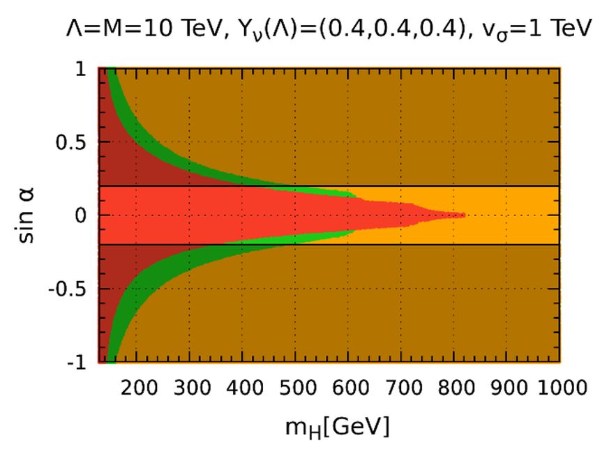
g1             g2          g3       yt          λSM
                          µ(mt )      0.462607         0.647737   1.16541    0.93519   0.126115

Table 1. MS values of the input parameters at the top quark mass scale, µ(mt ) = 173±0.4 GeV [3].

                          1.0
                                                                      SM
                          0.8                            g3
                                                 yt
                                g2

                                                                                                              JHEP03(2021)212
                          0.6
              Couplings

                                      g1
                          0.4

                          0.2
                                           λSM
                          0.0

                                103              106           109    1012          1015         1018
                                                                 μ [GeV]

Figure 1. The renormalization group evolution of the Standard Model gauge couplings g1 , g2 , g3 ,
the top quark Yukawa coupling yt and the quartic Higgs boson self-coupling λSM . Here we adopt
the MS scheme, taking the parameter values at low scale as input, see [5] for details.

gauge couplings g1 , g2 , g3 respectively, are the most important input parameters character-
izing the Standard Model renormalization group equations (RGEs). Given the values of
these input parameters,1 as shown in table 1, the Higgs quartic coupling tends to run
negative between the electroweak and Planck scales, as seen in figure 1.
     One sees that the Standard Model Higgs quartic coupling λSM becomes negative at
an energy scale ∼ 1010 GeV. This would imply that the Standard Model Higgs potential
is unbounded from below. Hence, the Standard Model vacuum is not absolutely stable [4,
6, 7]. Instead, these next-to-next-to-leading order analyses of the Standard Model Higgs
potential suggest that the vacuum is actually metastable.
     Moreover, despite its many successes, the Standard Model cannot be the final theory
of nature. One of its main shortcomings is its inability to account for neutrino mass gen-
eration, needed to describe neutrino oscillations [8]. The Higgs vacuum stability problem
in neutrino mass models can become worse than in the Standard Model [9–16]. Here we
follow ref. [5] and confine ourselves to the Standard-Model-based seesaw mechanism using
the simplest SU(3)c ⊗ SU(2)L ⊗ U(1)Y gauge group.
     The latter can be realized in “high-scale” schemes with explicit [17] or spontaneous vio-
   1
  The numbers given in table 1 are the central values. We use them as the input parameters for our
RGEs. The importance of errors has been studied in ref. [4], to which we refer the reader for more details.

                                                                –2–
Φ L Φ
Φ L Φ
Figure 2. Destabilizing effect of Weinberg’s effective operator on the Higgs quartic interaction.
lation of lepton number [18, 19]. These typicaly involve messenger masses much larger than
JHEP03(2021)212
the electroweak scale. Alternatively, neutrino mass may result from “low-scale” physics [20].
For example, the type-I seesaw mechanism can be mediated by “low-scale” messengers.
This happens in the inverse seesaw mechanism. Lepton number is broken by introducing
extra SU(3)c ⊗ SU(2)L ⊗ U(1)Y singlet fermions with small Majorana mass terms, in addi-
tion to the conventional “right-handed” neutrinos. Again, one can have either explicit [21]
or spontaneous lepton number violation [22].
Any theory with massive neutrinos has an intrinsic effect, illustrated in figure 2, that
may potentially destabilize the electroweak vacuum.2 This vacuum stability problem be-
comes severe in low-scale-seesaw schemes [5]. Indeed, if the heavy mediator neutrino lies in
the TeV scale, its Yukawa coupling will run for much longer than in the high-scale type-I
seesaw. As a consequence, the quartic coupling λ tends to become negative sooner, much
before the Standard Model instability sets in.
Here we examine the consistency of the electroweak symmetry breaking vacuum within
the inverse seesaw mechanism. Apart from the destabilizing effect illustrated in figure 2
there will in general be other, model-dependent, and possibly leading contributions that can
reverse this trend. We note that the spontaneous violation of lepton number, implying the
existence of a physical Nambu-Goldstone boson, dubbed majoron [18, 19], can substantially
improve the electroweak vacuum stability properties. Indeed, the extended scalar sector
of low-scale-majoron-seesaw schemes plays a key role in improving their vacuum stability.
This sharpens the results presented in ref. [11]. Indeed, we find that renormalization
group (RG) evolution can cure the vacuum stability problem in inverse seesaw models also
in the presence of threshold effects. These can be associated both with the scalar as well
as the fermion sector of the theory.3
The paper is organized as follows. In section 2, we describe neutrino mass generation
in the inverse-seesaw model. In section 3 we show that the vacuum stability problem
becomes worse within the simplest inverse-seesaw extensions with explicitly broken lepton
number. In section 4, we then focus on the majoron completion of the inverse seesaw. We
then show in section 5 how the majoron helps stabilize the Higgs vacuum, all the way up
to Planck scale. In section 6, we compare the vacuum stability properties of the various
missing-partner-inverse-seesaw variants with those of the sequential case. In section 7 we
2
In the presence of very specific symmetries this model-independent argument might be circumvented.
3
Notice that, while ref. [5] included threshold effects, in the high-scale seesaw framework such effects
appear only at high energies, and do not affect low-scale physics.
–3–briefly illustrate the interplay between vacuum stability and the restrictions on the Higgs
boson invisible decays [23] that follow from current LHC experiments. Finally, we conclude
and summarize our main results in section 8.
2 The inverse seesaw mechanism
The issue of vacuum stability must be studied on a model-by-model basis. In this work
we examine it in the context of inverse-seesaw extensions of the Standard Model. The
inverse seesaw mechanism is realized by adding two sets of electroweak singlet “left-handed”
fermions νic and Si [21, 22]. The relevant part of the Lagrangian is given by
JHEP03(2021)212
1
Yνij Li Φ̃νjc + M ij νic Sj + µij
X
−L = Si Sj + H.c. (2.1)
ij
2 S
T
where Li = ν ` ;i = 1, 2, 3 are the lepton doublets, Φ is the Standard Model Higgs
doublet, M is the Dirac mass term. The two sets of fields ν c and S transform under
the lepton number symmetry U(1)L as ν c ∼ −1 and S ∼ +1, respectively. The M and
µS terms are both gauge invariant mass matrices, but only M is invariant under lepton
number symmetry, since µS violates lepton number by two units. Light neutrino masses are
generated through the tiny lepton number violation. Indeed, after electroweak symmetry
breaking, the effective light neutrino mass matrix has the following form
0 mD 0
Mν = mTD 0 M , (2.2)
0 M T µS
with mD = √v Yν . Neutrino masses arise by block-diagonalizing eq. (2.2) as,
2
U T .Mν .U = MD (2.3)
through the unitary transformation matrix U , where MD has a block-diagonal form. Since
the lepton number is retored as µS → 0, the symmetry breaking entries of µS can be made
naturally small in the sense of t’Hooft. Apart from symmetry protection, the smallness
of µS may also result from having a radiative origin associated to new physics such as
supersymmetry, left-right symmetry or dark matter physics [24–26]. In contrast, being
gauge and lepton-number invariant, the elements of M are expected to be naturally large.
Thus we obtain the hierarchy M
mD
µS . Under this hierarchy assumption we
perform the standard seesaw diagonalization procedure [19], to obtain the effective light
neutrino mass matrix mν as
v2
mν ≈ mD M −1 µS (M T )−1 mTD = Yν M −1 µS (M T )−1 YνT (2.4)
2
Furthermore, in contrast to conventional type-I seesaw, the scale of lepton number vio-
lating parameter µS is much smaller than the characteristic mediators scale M . As a result,
–4–the heavy singlet neutrinos become quasi-Dirac-type fermions.4 Note that, the small lepton
number violating Majorana mass parameters in µS control the smallness of light neutrino
masses. As µS → 0, the global lepton number symmetry is restored, and as a result,
all the three light neutrinos are strictly massless. Small neutrino masses are “symmetry-
protected” by the tiny value of µS 6= 0. The smallness of µS allows the Yukawa couplings
Yν to be sizeable, even when the messenger mass scale M lies in the TeV scale, without
conflicting with the observed smallness of neutrino masses.
In contrast to the high-scale type-I seesaw, in inverse-seesaw schemes one can have
a very rich phenomenology that makes them potentially testable in current or upcoming
JHEP03(2021)212
experiments. For example, the mediators would be accessible to high-energy collider exper-
iments [28–31], with stringent bounds, e.g. from the Delphi and L3 collaborations [29, 30].
Moreover, they would induce lepton flavour and leptonic CP violating processes with po-
tentially large rates, unsuppressed by the small neutrino masses [32–36]. Finally, since the
mediators would not take part in low-energy weak processes, the light-neutrino mixing ma-
trix describing oscillations would be effectively non-unitary [37–41]. In short, in contrast
to the conventional high-scale seesaw, the inverse seesaw mechanism could harbor a rich
plethora of accessible new physics processes, that could be just around the corner.
As ν c and S’s are Standard Model gauge singlets, carrying no anomalies, there is
no theoretical limit on their multiplicity. Many possibilities can arise depending on the
number of ν c and S in a given model. In the sequential inverse seesaw model the number
of ν c matches that of S, and there are three “heavy” quasi-Dirac leptons in addition to
the three light neutrinos. For the case of different number of ν c and S, in addition to the
light and heavy neutrinos, the spectrum will also contain intermediate states with mass
proportional to µS . These could be warm dark matter candidate if their mass lies in KeV
scale [42].
For the sake of simplicity, here we consider only the case where ν c and S come with the
same multiplicity. Moroever, since adding more fermion species will only worsen the Higgs
vacuum stability problem, in section 3 we opt for the minimal (3,1,1) case, namely a single
pair of lepton mediators. In such minimal “missing-partner” seesaw [17] two of the light
neutrinos will be left massless. In section 6 we examine the quantitative differences between
the different multiplicity choices concerning the issue of vacuum stability. Moroever, we
briefly discuss the phenomenological viability of the various options.
3 Higgs vacuum stability in inverse seesaw
In the above preliminary considerations we have briefly summarized the main features of
the inverse seesaw model. We now examine the effect of the new fermions ν c and S upon
the stability of the electroweak Higgs vacuum. We take into account the effect of the
thresholds associated with the extra fermions ν c and S, as well as the scalars (in section 4
and 5) responsible for the spontaneous breaking of lepton number.
4
The concept of quasi-Dirac fermions was first suggested for the light neutrinos in [27]. It constitutes a
common feature of all low-scale seesaw models.
–5–3.1 Effective theory
To begin with, in the effective theory where the heavy singlet fermions ν c and S are
integrated out we have a natural threshold scale Λ ≈ M given by their mass, see eq. (2.1).
As as a result, below this scale the theory is the Standard Model plus an effective dimension
five Weinberg operator [43], given by
κ
−Ld=5
ν = L L Φ Φ + H.c. (3.1)
2
where κ = (Yν M −1 µS (M T )−1 YνT ) is the 3 × 3 effective coupling matrix. Unless they are
needed, in what follows we will suppress the generation indices. Note that κ has negative
JHEP03(2021)212
mass dimension. The above Lagrangian leads to a left-handed neutrino Majorana mass
matrix as
v2
mν ≡ κ (3.2)
2
As a result, below the scale Λ, only the Standard Model couplings and κ will run. Neglecting
lepton and light quark Yukawa couplings, the one-loop RGEs [44–46] are given by [5]
16π 2 βκ = 6yt2 κ − 3g22 κ + λκ κ (3.3)
Due to the large top Yukawa coupling, κ slowly increases with the threshold scale Λ.
We denote the Higgs quartic coupling in this case as λκ to distinguish it from the pure
Standard Model case. The above Weinberg operator also gives a correction to the Higgs
quartic coupling λκ below the scale Λ. The contribution of the coupling κ to the running
of λκ is of order v 2 κ2 and thus negligible, as shown in [5, 14, 46]. Hence, below the scale
Λ, the evolution of λκ will be almost the same as in the Standard Model.
3.2 Full theory
We now turn to the region above the threshold scale Λ. In this regime we have the full
Ultra-Violet (UV) complete theory. Hence one must take into account the RGEs of all the
new couplings present in the model, as they will affect the evolution of the Higgs quartic
coupling. In particular, we will see that the stability of the electroweak vacuum limits how
large the Yukawa coupling Yν can be. The Higgs quartic self-coupling in full UV-complete
theory will be denoted by λ, to distinguish it from the Standard Model coupling λSM and
from the effective theory quartic coupling λκ discussed above.
For simplicity we will first study the case of just one species of ν c and S, which we
call the (3, 1, 1) inverse seesaw. As mentioned, this of course is not — by itself — realistic,
as in this case only one of the light neutrinos obtains mass. However, the missing mass
parameter may arise from a different mechanism [26] associated, say, with dark matter.
Moreover, the (3, 1, 1) case provides the simplest reference scheme, that brings out all the
relevant features. In section 6 we will compare with the (3, 2, 2) and the (3, 3, 3) — the
sequential inverse seesaw mechanim — with two and three species of ν c and S, respectively.
The running of Yν above the threshold scale is governed by the RGEs given in ap-
pendix. A. Apart from the RG evolution, one must also take into account the threshold
–6–Λ=M=1 TeV, Yν (Λ)=0.6 Λ=M=100 TeV, Yν (Λ)=0.6
0.8 0.8
0.6 0.6
Yν Yν
Couplings
Couplings
0.4 0.4
0.2 0.2
λκ λκ
λSM λSM
0.0 0.0
λ λ
-0.2 3 6 9 12 15 18 -0.2 3 6 9
10 10 10 10 10 10 10 10 10 1012 1015 1018
JHEP03(2021)212
μ [GeV] μ [GeV]
Figure 3. Evolution of the Higgs quartic self-coupling λ (solid-red) and Yukawa coupling
Yν (dotted-green) within the minimal (3,1,1) inverse seesaw scheme. λκ is the quartic coupling
in the effective theory with the Weinberg operator. For comparison, we also plot the running of
λSM , the SM quartic coupling, indicated by the dashed-red line.
corrections, associated with integrating the heavy fermions in the effective theory. The
tree-level Higgs potential is given by
V = −µ2Φ (Φ† Φ) + λ(Φ† Φ)2 (3.4)
This will get corrections from higher loop diagrams of Standard Model particles as well
as from the extra fermions present in the inverse seesaw model. It introduces a threshold
correction to the Higgs quartic coupling λ at Λ = M . Here we follow ref. [5] in estimating
5 4
this threshold correction as ∆λTH = − 32π 2 |Yν | . We take into consideration this shift in λ
at Λ = M when solving the RGEs,
5
λ(Λ) → λ(Λ) − |Yν |4 . (3.5)
32π 2
Having set up our basic scheme, let us start by looking at the impact of the Yukawa
coupling Yν on the stability of the Higgs vacuum. As already discussed, in the Standard
Model, the running of the Higgs quartic coupling λSM is dominated by the top quark
Yukawa coupling and becomes negative around energy scale ∼ 1010 GeV. However, within
the inverse seesaw, the Yukawa coupling Yν in eq. (2.1) can dominate the evolution of λ
above the threshold scale Λ = M , as seen in figure 3.
In figure 3 we have shown the RG evolution of the relevant coupling parameters assum-
ing the Yukawa coupling Yν = 0.6 at the threshold scale, taken to be Λ = M = 103 GeV
(left panel) and 105 GeV (right panel). We see that λ becomes negative at around energy
scales 3.27 × 10⁷ GeV and 3.16 × 10⁸ GeV for the threshold scale Λ = 103 GeV and 105 GeV,
respectively. By comparing this with the running of the Standard Model Higgs quartic
coupling λSM (red dashed), one sees how the Higgs vacuum stability problem becomes
more acute in the inverse seesaw model. This was expected, since the new fermions tend to
destabilize the Higgs vacuum, as illustrated in figure 4. It should also be noted that in the
effective theory regime the evolution of the quartic coupling λκ almost coincides with that
–7–Φ νc Φ
L L
Φ νc Φ
JHEP03(2021)212
Figure 4. The destabilizing effect of right-handed neutrinos on the evolution of the Higgs quartic
coupling.
of λSM , due to the negligible effect of the Weinberg operator on its running. Finally, note
that all couplings in figure 3 remain within the perturbative region up to Planck scale.
Consistency restrictions. We now turn to the issue of the general self-consistency of the
inverse seesaw mechanism. In order to ensure a perturbative and mathematically consistent
model, the tree-level couplings must satisfy certain conditions, e.g. all of them should have
a perturbative value, and the potential should be bounded from below. However, once
we take into account the quantum corrections, these conditions also get corrected. In this
section we analyze these modified conditions in more detail.
We start by examining the restrictions coming from perturbativity at tree-level, which
√
require |Yν | < 4π. The RG evolution of Yν increases its value with increasing scale.
Figure 5 shows the evolution of Yν and λ. From the left panel of figure 5 one sees that
√
demanding that |Yν | < 4π up to the Planck scale implies that |Yν | . 0.8 at the threshold
scale Λ = 103 GeV. However, as one can see from figure 5, the Higgs quartic coupling
λ becomes negative much before the Planck scale. Therefore, demanding pertubativity
of Yν all the way up to the Planck scale does not ensure full consistency of the scalar
potential. If one demands perturbativity only till, say, 100 TeV, as shown in right panel of
figure 5, one finds that the pertubativity limit on Yν is relaxed to |Yν | . 2 at the threshold
scale Λ = 103 GeV. Such large Yν values lead to large threshold corrections for λ — the
negative jump shown in the right panel — making it negative even before turning on its
RG evolution.
This highlights the importance of taking into account the threshold corrections for λ.
From figure 5 one sees that a large Yν value can lead to an unbounded potential already at
the threshold scale, even before RG evolution. Taking the Yukawa coupling Yν (Λ) = 1.58
at Λ = 103 GeV makes λ(Λ) = 0 due to threshold corrections. RG running will further
decrease λ above the threshold scale, making the vacuum unstable. It is clear that threshold
corrections are crucial when considering large Yukawa couplings and that a true limit on
Yν requires one to take into account both RG evolution as well as the threshold corrections
it induces on the quartic coupling λ.
As an example, in figure 6 we show the result of demanding that neither Yν goes
non-perturbative, nor λ goes negative up to 100 TeV. To quantify the implications of this
–8–Λ=M=1 TeV, Yν (Λ)=0.84 Λ=M=1 TeV, Yν (Λ)=2
3 3
Yν
2 Yν
2
1
Couplings
Couplings
1
λκ
0 λκ
λ
0
-1
-1 λ
-2
-2
-3
-3
103 106 109 1012 1015 1018 103 104 105
JHEP03(2021)212
μ [GeV] μ [GeV]
√
Figure 5. Perturbativity limits on the Yukawa coupling Yν . The left panel requires Yν < 4π up
√
to the Planck scale, so that only RG evolution is relevant. The right panel demands Yν < 4π only
up to 100 TeV. In this case Yν is large enough that threshold effects make λ negative even before
running. In both cases the vacuum is unstable, i.e. λ < 0, before Yν reaches the perturbative limit,
see text for details.
Λ=M=1 TeV, Yν (Λ)=0.87
Λ=M=10 TeV, Yν (Λ)=1.02
1.0
Yν 1.0 Yν
0.8
0.8
Couplings
Couplings
0.6
0.6
0.4
0.4
0.2 λκ 0.2 λκ
λ λ
0.0 0.0
103 104 105 103 104 105
μ [GeV] μ [GeV]
Figure 6. Limiting Yν by demanding Yν to remain perturbative and λ to remain positive up to
100 TeV. Left (right) panel correspond to threshold scales Λ = 1 TeV (Λ = 10 TeV). See text for
details.
demand, we have taken two threshold scales, Λ = 103 GeV (left panel), and Λ = 104 GeV
(right panel), respectively. With this combined requirement we obtain the limit Yν . 0.87
(left panel) and Yν . 1.02 (right panel). This illustrates that the limit on Yν also depends
on the choices of threshold scale, for higher threshold scales the limit on Yν gets relaxed.
4 The majoron completion of the inverse seesaw
In the previous section we saw that the addition of new fermions to the Standard Model
in order to mediate neutrino mass generation via the inverse seesaw mechanism [21] has a
destabilizing effect on the Higgs vacuum. This problem can be potentially cured if there
are other particles in the theory providing a “positive” contribution to the RGEs governing
–9–the evolution of the Higgs quartic coupling. A well-motivated way to do this is to assume
the dynamical version of the inverse seesaw mechanism [22].
Building up on the work of ref. [11] here we focus on low-scale generation of neutrino
mass through the inverse seesaw mechanism with spontaneous lepton number violation.
Lepton number is promoted to a spontaneously broken symmetry within the minimal
SU(3)c ⊗ SU(2)L ⊗ U(1)Y gauge framework. To achieve this, in addition to the Stan-
dard Model singlets ν c and S, we now add a complex scalar singlet σ carrying two units
of lepton number. Lepton number symmetry is then spontaneously broken by the vacuum
expectation value of σ. The relevant Lagrangian is given by
JHEP03(2021)212
3
Yνij Li Φ̃νjc + M ij νic Sj + YSij σSi Sj + H.c.
X
−L = (4.1)
i,j
After the electroweak and lepton number symmetry breaking the neutrino mass matrix has
the following form
0 mD 0
T
Mν = mD 0 M (4.2)
0 M T µS
where mD = Y√ ν vΦ
2
, µS = 2 Y√
S vσ
2
vΦ
with hΦi = √ 2
vσ
and hσi = √ 2
being the vacuum expecta-
tion values (vevs) of the Φ and σ fields respectively. Again, within the standard seesaw
approximation, the effective neutrino mass is obtained as
v2
mν ' √Φ Yν M −1 YS vσ (M T )−1 YνT (4.3)
2
Light neutrino masses of O(0.1) eV, are generated for reasonable choices of vσ and M ,
small Yukawa couplings YS , and sizeable Yν ∼ O(1).
Turning to the scalar sector, in the presence of the complex scalar singlet σ and dou-
blet Φ, the most general potential driving electroweak and lepton number symmetry break-
ing is given by
V = −µ2Φ Φ† Φ − µ2σ σ † σ + λΦ (Φ† Φ)2 + λσ (σ † σ)2 + λΦσ (Φ† Φ)(σ † σ). (4.4)
As already noted, in addition to the SU(3)c ⊗ SU(2)L ⊗ U(1)Y gauge invariance, V (Φ, σ)
also has a global U(1) lepton number symmetry.
√
This potential is bounded from below if λσ , λΦ and λΦσ + 2 λσ λΦ are all positive,
and has a minimum for non-zero vacuum expectation values of both Φ and σ provided λΦ ,
λσ and 4λΦ λσ − λ2Φσ are all positive. After the breaking of electroweak and lepton number
symmetries, we end up with a physical Goldstone boson, the Majoron J [18, 19], which is
a pure gauge singlet. After symmetry breaking one has, in the unitary gauge,
!
1 0 vσ + σ 0 + iJ
Φ→ √ , σ→ √ . (4.5)
2 v Φ + h0 2
– 10 –The CP even fields h0 and σ 0 will mix, so the mass matrix for neutral scalar Mns is given by
!
2 λ v v
2λΦ vΦ
2 Φσ Φ σ
Mns = (4.6)
λΦσ vΦ vσ 2λσ vσ2
We can diagonalise the above mass matrix to obtain the mass eigenstates (h H)T through
the rotation matrix OR as
! ! ! !
h h0 cos α sin α h0
= OR ≡ , (4.7)
H σ0 −sin α cos α σ0
JHEP03(2021)212
Here α is the CP-even scalar mixing angle, and its range of allowed values is constrained
by LHC data [47, 48]. The rotation matrix satisfies
2 T
OR Mns OR = diag(m2h , m2H ) (4.8)
where the masses mh , mH of the scalars h, H respectively, are given by
q
m2h = λΦ vΦ
2
+ λσ vσ2 − 2 − λ v 2 )2 + (λ vv )2
(λΦ vΦ σ σ Φσ σ (4.9)
q
m2H = λΦ vΦ
2
+ λσ vσ2 + 2 − λ v 2 )2 + (λ vv )2
(λΦ vΦ σ σ Φσ σ (4.10)
The lighter of these two mass eigenstates h is identified with the 125 GeV scalar discovered
at the LHC [1, 2].
We can use eqs. (4.9) and (4.10) along with (4.6)–(4.7) to solve for the parameters λΦ ,
λσ and λΦσ in terms of physical quantitites i.e. masses m2h , m2H and the mixing angle α as
m2h cos2 α + m2H sin2 α
λΦ = 2 , (4.11)
2vΦ
m2h sin2 α + m2H cos2 α
λσ = , (4.12)
2vσ2
(m2h − m2H ) sin α cos α
λΦσ = . (4.13)
vΦ vσ
5 Vacuum stability in inverse seesaw with majoron
In this section we will explore the consequences of spontaneous breaking of the lepton
number symmetry on the stability of the electroweak vacuum. Due to the presence of the
scalar σ, the RGE of the Φ quartic coupling receives a new 1-loop contribution through the
diagram shown in figure 7. This “positive” contribution plays a crucial role in counteracting
the “negative” contribution coming from the extra fermions of the inverse seesaw model,
see figure 4.
Vacuum stability in this model can be studied in two different regimes namely
(i) vσ
vΦ and (ii) vσ ≈ O(vΦ ). We start with the first possibility. As before, we fo-
cus on the missing partner (3, 1, 1) inverse seesaw, other possibilities will be taken up in
section 6.
– 11 –Φ Φ
σ σ
Φ Φ
Figure 7. One-loop correction to the Φ quartic coupling due to its interaction with the singlet σ
JHEP03(2021)212
that drives spontaneous lepton number violation in inverse seesaw models. This diagram leads to
a “positive” term in the RGE of the Φ quartic coupling, that can overcome the destabilizing effect
of the fermions in figure 4.
5.1 Case I: vσ
vΦ
In the limit vσ
vΦ the heavy CP-even Higgs boson H almost decouples, with its mass
√
mH given as mH ≡ MH ≈ 2λσ vσ . Moreover, in this limit small neutrino masses require
small YS , so the two heavy singlet fermions ν c and S form a quasi-Dirac pair with nearly
degenerate mass M . We assume, for simplicity of the analysis, that MH and M , have a
common value, so that we deal with just one threshold scale Λ = M = MH . Below this
scale we have an effective theory with the Standard Model structure, suplemented by the
Weinberg operator for neutrino mass generation.5 Thus, below the threshold scale, we need
√
to integrate out 2Re(σ) at tree-level [49]. As a result, at the scale Λ, there is a tree-level
λ2Φσ
threshold correction which induces a shift in the Higgs quartic coupling, δλ = 4λσ . This
will lead to the following effective Higgs potential below the threshold scale Λ
!2
v2
Veff = λ0Φ Φ† Φ − , (5.1)
2
where the effective Higgs quartic coupling λ0Φ below the threshold scale is defined as
λ2Φσ
λ0Φ ≡ λκ = λΦ − . (5.2)
4λσ
Here λκ is the effective quartic coupling for the case of explicit lepton number breaking,
see section 3. The evolution of the Higgs quartic coupling λ0Φ in the effective theory is
shown in figure 8. One can appreciate the jump in the value of the Higgs quartic coupling
due to threshold corrections. Since only the dimension-five Weinberg operator runs below
the scale Λ, the RG evolution of λSM is essentially the same as that of λ0Φ . Both are very
close to the RG running of λκ of the effective theory with explicit lepton number breaking.
Moreover, at tree-level the numerical value of λκ (MZ ) and λSM (MZ ) is the same, since in
both cases one must reproduce the 125 GeV Higgs mass.
Moving on to the full theory at the threshold scale Λ = M , the first thing to note is
the impact of threshold corrections, eq. (5.2). They lead to a positive shift in value of the
5
Note that the majoron J will also be present in this effective theory. Even though massless or fairly
light, it will pratically decouple from the Higgs boson, and will not affect vacuum stability.
– 12 –Λ=M=mH =10 TeV, Yν (Λ)=0.45, λσ (Λ)=λΦσ (Λ)=0.1 Λ=M=mH =100 TeV, Yν (Λ)=0.45, λσ (Λ)=λΦσ (Λ)=0.1
0.6 0.6
0.5 0.5
Yν Yν
0.4 0.4
Couplings
Couplings
0.3 0.3
0.2 λΦσ 0.2
λΦσ
λΦ' λσ λΦ' λσ
0.1 0.1
λΦ λΦ
0.0 0.0
λSM λSM
- 0.1 3 6 9 12 15 18 - 0.1 3 6 9 12 15
10 10 10 10 10 10 10 10 10 10 10 1018
JHEP03(2021)212
μ [GeV] μ [GeV]
Figure 8. The RG evolution of the quartic couplings and right-handed neutrino Yukawa couplings
within the Majoron extension of (3,1,1) inverse seesaw scheme. For comparison, we also show the
evolution of λSM (red-dashed). Here λ0Φ ≡ λκ is the effective Higgs quartic coupling below threshold,
see eq. (5.2).
Higgs quartic coupling above the threshold scale Λ = M , enhancing the chances of keeping
λΦ positive [5]. Furthermore, to understand the evolution of λΦ in the full theory above
the scale Λ = M one must perform the RG evolution of all parameters. Above the scale
Λ one needs to include βλΦσ , βλσ and evolve the quartic coupling λΦ using the full RGEs
with the matching condition eq. (5.2) at Λ. In appendix. B, we give the two-loop RGEs of
the full theory.
In figure 8 we show the evolution of various couplings in the majoron inverse seesaw
model for given benchmark points. We have taken the threshold scale as M = MH = 10 TeV
and M = MH = 100 TeV for the left and right panels, respectively. For the sake of
comparison, the initial values of other parameters have been kept the same in both panels.
The Yukawa coupling has been fixed at Yν = 0.45. We have taken λσ , λΦσ = 0.1 at the
scale Λ. The positive shift in the evolution of λ at the threshold scale is coming from the
matching condition given in eq. (5.2). Notice that below threshold the running of λ0Φ and
λSM almost coincide with each other, due to the tiny effective Weinberg operator. Finally,
since YS has been taken to be very small, it has no direct impact on vacuum stability.
In summary, it is clear from figure 8 that the dynamical variant of the inverse seesaw
mechanism can be free from the Higgs vaccum instability problem. This is possible thanks
to the positive contribution of the scalar σ both to the threshold corrections, as well as to
the RG evolution of the Higgs quartic coupling. These effects are enough to counteract the
negative contribution of the new fermions present in inverse seesaw model, even for sizeable
Yukawa couplings Yν ∼ O(1). These could lead to a plethora of new phenomena [28–41].
Thus, in contrast to the case of inverse seesaw with explicitly broken lepton number, the
dynamical variants can have a completely stable Higgs vacuum.
5.2 Case II: vσ = O(vΦ )
In this case, the mass of the heavy scalar mH is of the order of the electroweak scale. Hence
we can neglect the small range between MZ and mH , starting instead with eq. (4.13), which
– 13 –Λ=M=10 TeV, Yν (Λ)=0.5, mH =400 GeV, α=0.2, vσ =1 TeV Λ=M=100 TeV, Yν (Λ)=0.6, mH =400 GeV, α=0.2, vσ =1 TeV
0.8 0.8
0.6 Yν
0.6 Yν
Couplings
Couplings
0.4 0.4
0.2 λΦ λΦσ 0.2 λΦ λΦσ
λσ λσ
0.0 0.0
λSM λSM
103 106 109 1012 1015 1018 103 106 109 1012 1015 1018
JHEP03(2021)212
μ [GeV] μ [GeV]
Λ=M=10 TeV, Yν (Λ)=0.5, mH =800 GeV, α=0.1, vσ =3 TeV Λ=M=100 TeV, Yν (Λ)=0.6, mH =800 GeV, α=0.1, vσ =3 TeV
0.8 0.8
0.6 Yν
0.6 Yν
Couplings
Couplings
0.4 0.4
0.2 λΦ λΦσ 0.2 λΦ λΦσ
λσ λσ
0.0 0.0
λSM λSM
103 106 109 1012 1015 1018 103 106 109 1012 1015 1018
μ [GeV] μ [GeV]
Figure 9. Evolution of the quartic couplings and right-handed neutrino Yukawas within the
Majoron extension of the missing partner (3,1,1) inverse seesaw scheme. For comparison, the
evolution of λSM is shown in the red dashed curve. Here only the fermion singlets are integrated
out at the threshold scale Λ = M , all scalars are part of the effective theory below threshold, taken
as the weak scale.
already includes the threshold effect of eq. (5.2). Thus in this case only the fermions are
integrated out at the threshold scale Λ = M , while all the scalars remain in the resulting
theory below threshold. Thus the scalar couplings evolve over a larger range, and have
better chance of curing the Higgs vacuum instability problem. Needless to say that, as
before, the Higgs vaccum instability can be avoided if the mixed quartic λΦσ is sufficiently
large, O(0.1). This in turn implies a sizeable mixing α ∼ O(0.1) between the two CP-even
Higgs bosons.
The evolution of the couplings in this case is shown in figure 9. In these plots, we
have fixed the singlet neutrino scale Λ = 10 TeV in the left panel, and 100 TeV in the
right panel. In contrast to the scalar couplings, the Yukawa coupling Yν starts running
only above threshold. Notice that for relatively large mediator scale, the allowed value
of Yν will also be large as there is not enough range, in terms of RGEs evolution, to
sizeably alter the Yν . We found that for large Yukawa couplings, Yν ≥ 0.7 (0.8) for
threshold scale Λ = 10 TeV (100 TeV), respectively, we get either unstable vacuum or non-
perturbative dynamics.
– 14 –Moreover, as shown in figure 9, we can have positive λΦ , λσ and λΦσ all the way up
to the Planck scale, even for sizeable Yukawa couplings. We found that for small mH the
required mixing angle is relatively large, in contrast to the large mH case. For small α
or mH the potential becomes unbounded from below at high energies. In other words,
experimental limits on α, e.g. coming from the LHC [47, 48], can be used to place a lower
limit on the mass mH . In section 7 we illustrate the interplay between the vacuum stability
restrictions and the constraints on the invisible width of the Higgs boson that follow from
current LHC experiments. There we also note that in order to prevent the existence of
Landau poles in the running parameters, the lepton number breaking scale vσ should not
be too small.
JHEP03(2021)212
6 Comparing sequential and missing partner inverse seesaw
For simplicity we have so far only analyzed the explicit and dynamical lepton number
breaking within the simplest (3,1,1) missing partner inverse seesaw mechanism. We now
compare the stability properties of this minimal construction with those of (3,2,2) and
(3,3,3) inverse seesaw mechanisms.
6.1 Sequential versus missing partner seesaw: electroweak vacuum stability
As already mentioned, the problem of Higgs vacuum stability only gets worse with the
addition of extra fermions. This fact is clearly illustrated in figure 10 where we compare
the RG evolution of the Higgs quartic coupling λ within the Standard Model (dashed, red)
with the (3, n, n) inverse seesaw completions, with n = 1 (solid, blue), n = 2 (dot-dash,
magenta) and n = 3 (dot, green).
In figure 10 we have taken the initial Yukawa coupling values in such a way as to
facilitate a proper comparison of the different cases. To do this for (3,1,1) case, we have
fixed the Yukawa coupling |Yν | = 0.4. For (3,2,2) and (3,3,3) case, we have taken the
diagonal entries of the Yν matrix to be Yνii = 0.4, while all off-diagonal ones, Yνij for i 6= j,
were neglected in the RGEs. Clearly one sees how (3, n, n) inverse seesaw scenarios with
n > 1 have worse Higgs vacuum stability properties than the n = 1 case.
In figure 11, we display our vacuum stability results for the majoron inverse seesaw
models. One can compare the Standard Model case (dashed, red) with the (3,1,1) (solid,
blue), (3,2,2) (dot-dash, magenta) and (3,3,3) (dot, green) majoron inverse seesaw schemes.
As before, to ensure a consistent comparison, we have taken the Yukawa coupling |Yν | = 0.4
for (3,1,1) case, while for the (3,2,2) and (3,3,3) cases, we have taken Yνii = 0.4 and neglected
off-diagonal Yνij . In the left panel we have taken the case of Λ = M = mH = 10 TeV. Below
√
threshold we have integrated out the fields 2Re(σ), ν c and S and included the threshold
effects. This leads to the jump in the quartic coupling seen in the figure. In contrast, for
the right panel, we have fixed vσ = 1 TeV and mH = 500 GeV. In this case the scalars
are not integrated out and the quartic coupling runs smoothly from electroweak scale till
Planck scale.
Figure 11 clearly illustrates that even for n ≥ 2, we can have a stable electroweak
vacuum for adequate choices of α and mH . Indeed, even in the higher (3,2,2) and (3,3,3)
– 15 –0.15
(3, 3, 3)
(3, 2, 2)
0.10 (3, 1, 1)
SM
0.05
λ
0.00
- 0.05
- 0.10
JHEP03(2021)212
103 106 109 1012 1015 1018
μ [GeV]
Figure 10. Comparing the evolution of the quartic Higgs self-coupling λ in the Standard Model
(dashed, red) with various inverse-seesaw extensions with explicit lepton number violation: (3,1,1)
denoted in solid (blue), (3,2,2) dot-dashed (magenta) and (3,3,3) dotted (green), see text for details.
Λ=M=mH =10 TeV, λσ (Λ)=0.1, λΦσ (Λ)=0.12 Λ=M=10 TeV, mH =500 GeV, α=0.12, vσ =1 TeV
0.15 0.20
(3, 3, 3) (3, 3, 3)
(3, 2, 2) 0.15 (3, 2, 2)
0.10 (3, 1, 1) (3, 1, 1)
SM 0.10 SM
λΦ
λΦ
0.05 0.05
0.00
0.00
- 0.05
- 0.05 - 0.10
103 106 109 1012 1015 1018 103 106 109 1012 1015 1018
μ [GeV] μ [GeV]
Figure 11. Comparing the evolution of the quartic Higgs self-coupling λ in the Standard Model
(red dashed) with the majoron inverse seesaw mechanism: the minimal (3,1,1) is denoted in solid
(blue), (3,2,2) is dot-dashed (magenta) and (3,3,3) is dotted (green). See text for details.
majoron inverse seesaw, the positive contribution from the new scalar is enough to overcome
the negative contribution from the new fermions of the inverse seesaw. In short, the Higgs
vacuum can be kept stable all the way up to the Planck scale even for appreciable Yukawa
coupling Yν .
6.2 Sequential versus missing partner seesaw: brief phenomenological discus-
sion
Here we note that neither the explicit nor the dynamical variant of the minimal (3,1,1)
inverse seesaw mechanism is phenomenologically realistic. The reason is that (3,1,1) leads
to only one massive neutrino (lying say, at the atmospheric scale), hence inconsistent with
oscillation data [8]. This minimal scheme is simply the inverse seesaw embedding of the
minimum “missing partner” (3,1) see saw mechanism of section III in ref. [17]. This lack
of the solar neutrino mass splitting can be avoided by the presence of a complementary
– 16 –radiative mechanism. To implement such “radiative completion” of the minimal scheme one
would need to invoke new physics. The latter could be associated, say, to the presence of a
dark matter sector [50]. This would provide an elegant theory with a tree-level atmospheric
scale, and a radiatively-induced solar neutrino mass scale, very much analogous to the case
of the bilinear breaking of R-parity in supersymmetry [51–53].
Alternatively, one can generate non-zero tree-level masses for two neutrinos by going
directly to the (3,2,2) “missing partner” seesaw scheme. Again, this would be the inverse-
seesaw-analogue of the (3,2) seesaw mechanism in ref. [17]. Finally, the sequential (3,3,3)
inverse seesaw mechanism will generate tree-level masses for all three light neutrinos. Any
of these would be totally consistent with neutrino oscillations.6
JHEP03(2021)212
Concerning neutrinoless double beta decay, here lies an important phenomenological
difference between the “missing partner” and the “sequential” seesaw mechanism. In the
missing partner seesaw there can be no cancellation amongst the individual light-neutrino
amplitudes leading to the decay [54].7 As a result, there is a lower bound on the neutrinoless
double beta decay rates that could be testable in the upcoming generation of searches.
There are other implications of low-scale seesaw schemes, such as our inverse-seesaw,
that could be potentially testable in current or upcoming experiments. For example, the
associated heavy neutrino mediators could be accessible at high energy experiments such as
e+ e− collider [28–31], with stringent bounds, e.g. from the Delphi and L3 collaborations [29,
30]. Likewise, they could produce interesting signatures at the LHC [58, 59]. Moreover,
these mediators would also induce lepton flavour and leptonic CP violation effects with
potentially detectable rates, unsuppressed by the small neutrino masses [32–36]. Finally,
since the heavy singlet neutrinos would not take part in oscillations, these could reveal new
features associated to unitarity violation in the lepton mixing matrix [37–41]. A dedicated
study would be required to scrutinize whether these signatures could be used to distinguish
missing partner from sequential seesaw.
7 Impact of invisible Higgs decay on the vacuum stability
As we saw above, vacuum stability is often threatened by the violation of the condition
λΦ > 0. From the RGE running of λΦ in eq. (B.1) one sees that in order to overcome
the destabilizing effect coming from fermions (−6yt4 and −2Tr(Yν Yν† Yν Yν† )), one needs a
relatively large mixed quartic coupling λΦσ . This in turn translates into a large mixing
angle α between the CP -even neutral Higgs bosons h and H. We see from eq. (4.13) that
large λΦσ implies smaller mixing angle | sin α| for larger mH and vice-versa. Within dy-
namical low-scale seesaw schemes with vσ ∼ O(TeV), relatively large mixing angle | sin α| is
expected. This is in potential conflict with the invisible Higgs decay constraints from LHC.
Indeed, it has long been noted that models with spontaneous violation of global sym-
metries such as lepton number at low scales vσ ∼ O(TeV) lead to sizeable invisible Higgs
decays, i.e. h → JJ [23] where J is the Majoron. The existence of such invisible decays
6
Modulo, of course, explaining the detailed pattern of mixing angles indicated by the oscillation data [8].
Such a challenging task would require a family symmetry, whose detailed nature is not yet fully understood.
7
This feature may also be implemented in some radiative schemes of scotogenic type, see e.g. [55–57].
– 17 –JHEP03(2021)212
Figure 12. Values of mH and mixing angle α leading to a stable potential (green), an unstable
potential (red) and non-perturbative dynamics (orange). Here we take the (3,1,1) missing partner
majoron inverse seesaw as the reference, with the heavy fermion threshold scale fixed as Λ = 10 TeV,
Yukawa coupling Yν = 0.4 and vσ = 1 TeV. Within the green region all couplings are perturbative
and the vacuum is stable up to the Planck scale. In the red region the potential becomes unbounded
from below before the Planck scale. The orange region has nonperturbative couplings (including
Landau poles) at energy scales below the Planck scale. The region outside the horizontal band
delimited by the black lines is ruled out by the LHC constraints on invisible Higgs decays. More
details in text.
can be probed by the LHC experiments [47, 60, 61]. The tightest bound on invisible Higgs
boson decays comes from the CMS experiment at the LHC, BR(h → Invisible) ≤ 19% [62].
This upper limit on the invisible Higgs decay sets a tight constraint on λΦσ or | sin α| for
mH > 130 GeV. For example with vσ = 1 TeV one gets | sin α| < 0.2 for mH > 130 GeV.
So far in all of our discussions we have chosen the mixing angle | sin α| for fixed vσ and
mH in such a way that one has consistency with the CMS constraint on invisible Higgs
decay. However, the full parameter space of the model contains regions consistent with
vacuum stability but disallowed by the invisible Higgs decay constraints. We illustrate this
in figure 12 for the (3,1,1) missing partner seesaw with relatively large Yukawa coupling
Yν = 0.4. Figure 12 shows the values of mH and α for vσ = 1 TeV which lead to either
stable/unstable potential or non-perturbative dynamics, as follows:
• Green Region: in this region we have a stable vacuum all the way up to the Planck
scale, with all the couplings within the perturbative regime. In our numerical scan
these conditions are implemented in following ways: 0 < λΦ (µ) < 4π, 0 < λσ (µ) < 4π,
p
λΦσ (µ) + 2 λΦ (µ)λσ (µ) > 0, |λΦσ (µ)| < 4π and |Yν (µ)| < 4π where µ is the running
mass scale.
• Red Region: in this region the potential becomes unbounded from below at some
high energy scale before the Planck scale. The potential is unbounded from below
if any (or more) of the following conditions is realised: λΦ (µ) ≤ 0, λσ (µ) ≤ 0 or
p
λΦσ (µ) + 2 λΦ (µ)λσ (µ) ≤ 0.
– 18 –• Orange Region: here one or more couplings become non-perturbative below the
Planck scale. This happens if any one of the following conditions holds: |λΦ (µ)| ≥ 4π,
|λσ (µ)| ≥ 4π, |λΦσ (µ)| ≥ 4π, |Yν (µ)| ≥ 4π. Note that the possibility of Landau poles
is also included inside the non-perturbative regions.
• Collider constraint: this is the region disallowed due to the LHC restriction on
the Higgs invisible decay branching fraction which requires BR(h → Invisible) ≤
19% [62].
From figure 12 one sees that for small mH , the required mixing angle is large, in order to
JHEP03(2021)212
ensure a stable electroweak vacuum. This is in turn in conflict with the invisible Higgs
decay constraints. As a result, one sees that these constraints are complementary to the
vacuum consistency requirements of pertubativity and stability. Altogether, these can rule
out a large part of the model parameter space.
The above discussion refers to our (3,1,1) majoron inverse seesaw reference case, tem-
plate for the scoto-seesaw mechanism [50]. One may now wonder how this discussion will
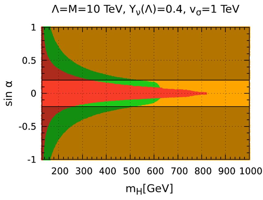
change in the higher (3, n, n); n ≥ 2 inverse seesaw schemes which do not require a “com-
pletion” so as to generate the atmospheric scale. In figure 13 we display the results for
the (3,2,2) (left panel) and (3,3,3) (right panel) scenarios. As expected, the undesired
effect of additional fermions on the stability of the vacuum is clearly visible. Indeed, the
unstable red regions in figure 13 are larger than in figure 12. Likewise, the same effect
is seen by comparing the left and right panels of figure 13. It is clear from figure 12 and
figure 13 that the allowed parameter space consistent with stability and LHC constraints
in the (3, n, n) seesaw with n ≥ 2 is more tightly restricted than in our reference n = 1
case. However we note that, for moderate values of the Yukawa coupling, we still have
parameter regions where electroweak breaking is consistent with the LHC measurements.
Although in the above we discussed (3,1,1), (3,2,2) and (3,3,3) cases separately, one should
note that, in terms of RGE evolution, there is not much difference between them. The
corresponding RGEs (see appendix) are the same by replacing |Yν |2 by Tr(Yν† Yν ). Hence
as long as one takes |Yν |2 ≈ Tr(Yν† Yν ), the (3,1,1) and (3, n, n) with n ≥ 2 schemes are
effectively the same.
Note that the restriction on the mixing angle gets stronger for lower values of vσ and
weakens for higher values of vσ , disappearing for high enough vσ . Therefore, the LHC
measurements constitute a probe of the lepton number violation scale vσ associated to
neutrino mass generation. Moreover, note that here we have only considered the case when
the lighter of the two CP even scalars is identified as the 125 GeV Higgs boson. A priori,
the possibility that the heavier CP even scalar is the 125 GeV Higgs boson should also be
discussed. Finally, in the discussions of figure 12 and figure 13 we have required vacuum
stability and perturbativity all the way up to the Planck scale. This will be an over-
requirement, if there is other new physics at play. In that case one should require vacuum
stability and perturbativity only up to a lower energy scale, say only up to 100 TeV, thus
relaxing the resulting restrictions. All of these issues require a dedicated study, that lies
beyond the scope of the present work.
– 19 –JHEP03(2021)212
Figure 13. Vacuum consistency constraints of figure 12 for the case of (3,2,2) (left) and
(3,3,3) (right) inverse majoron seesaw mechanism. The diagonal entries of the Yν matrix are fixed
as Yνii = 0.4. See text.
8 Conclusions
We have examined the consistency of electroweak symmetry breaking within the inverse
seesaw mechanism. We have derived the full two-loop renormalization group equations
of the relevant parameters within inverse seesaw schemes, examining both the simplest
inverse seesaw with explicit violation of lepton number, as well as the majoron extension
of inverse seesaw. The addition of fermion singlets (ν c and S) has a destabilizing effect
on the running of the Higgs quartic coupling λ. We found that for the inverse seesaw
mechanism with sizeable Yukawa coupling Yν the quartic coupling λ becomes negative
much before the Standard Model instability scale ∼ 1010 GeV. We have taken as our
simplest benchmark neutrino model the “incomplete” (3,1,1) inverse seesaw scheme, as
it has the “best” stability properties within this class of seesaw schemes. We compared
this reference case, in which only one oscillation scale is generated at tree-level, with the
“higher” inverse seesaw constructions (3, n, n) with n = 2, 3, in which other mass scales,
such as the atmospheric scale, also arise from the tree-level seesaw mechanism. Our main
results on the stability of the electroweak vacuum are summarized in figures 3, 8, 9, 10
and 11. We showed how, in contrast to simplest inverse seesaw with explicit lepton number
violation, the stability properties improve when this violation is spontaneous, and there is
a physical Nambu-Goldstone boson, the majoron. The comparison with LHC restrictions
is given in figures 12 and 13. We found that the LHC measurements constitute a probe of
the lepton number violation scale vσ associated to neutrino mass generation. Its detailed
study, however, needs further investigation. For example, we have assumed the lighter
of the two CP even scalars to be the 125 GeV Higgs boson. The alternative intriguing
possibility should a priori also be considered. We have also required vacuum stability and
perturbativity all the way up to the Planck scale. This is clearly an over-requirement, in the
presence of additional new physics. The latter could be associated say, to dark matter or to
the strong CP problem. In such case one should require vacuum stability and perturbativity
only up to a lower intermediate energy scale, thus relaxing the restrictions we have obtained.
All of these issues require a dedicated study, that lies beyond the scope of the present work.
– 20 –You can also read