Model of Anisotropic Reverse cardiac Growth in Mechanical Dyssynchrony
←
→
Page content transcription
If your browser does not render page correctly, please read the page content below
www.nature.com/scientificreports

                        OPEN       Model of Anisotropic Reverse
                                   Cardiac Growth in Mechanical
                                   Dyssynchrony
Received: 21 February 2019         Jayavel Arumugam1, Joy Mojumder1, Ghassan Kassab2 & Lik Chuan Lee1
Accepted: 9 August 2019
Published: xx xx xxxx              Based on recent single-cell experiments showing that longitudinal myocyte stretch produces both
                                   parallel and serial addition of sarcomeres, we developed an anisotropic growth constitutive model with
                                   elastic myofiber stretch as the growth stimuli to simulate long-term changes in biventricular geometry
                                   associated with alterations in cardiac electromechanics. The constitutive model is developed based on
                                   the volumetric growth framework. In the model, local growth evolutions of the myocyte’s longitudinal
                                   and transverse directions are driven by the deviations of maximum elastic myofiber stretch over a
                                   cardiac cycle from its corresponding local homeostatic set point, but with different sensitivities. Local
                                   homeostatic set point is determined from a simulation with normal activation pattern. The growth
                                   constitutive model is coupled to an electromechanics model and calibrated based on both global and
                                   local ventricular geometrical changes associated with chronic left ventricular free wall pacing found
                                   in previous animal experiments. We show that the coupled electromechanics-growth model can
                                   quantitatively reproduce the following: (1) Thinning and thickening of the ventricular wall respectively
                                   at early and late activated regions and (2) Global left ventricular dilation as measured in experiments.
                                   These findings reinforce the role of elastic myofiber stretch as a growth stimulant at both cellular level
                                   and tissue-level.

                                   Mechanical dyssynchrony of the heart such as left bundle branch block (LBBB) is caused by the asynchronous
                                   electrical activity of the left ventricle (LV) through slow conduction across the myocytes instead of through the
                                   fast conduction Purkinje system. Besides acute changes like QRS prolongation, reduction in wall motion and
                                   changes in blood flow1, abnormal contraction of the dyssynchronous heart can lead to long-term ventricular
                                   remodeling if left untreated. Patients with LBBB not only have an increased risk of developing cardiac disease2,
                                   such as hypertension, congestive heart failure, but also have a higher mortality rate2–4. Experimental studies using
                                   animal models have shown that ventricular pacing, which induces an asynchronous electrical activation and
                                   contraction pattern, produces both global and local LV remodeling in the form of ventricular dilation and asym-
                                   metrical hypertrophy, respectively5.
                                       Computational modeling is increasingly used to simulate long-term changes associated with cardiac growth.
                                   Formulated based on the volumetric growth framework in which the deformation gradient tensor is multiplica-
                                   tively decomposed into an elastic and a growth component6,7, cardiac growth constitutive models are developed
                                   to phenomenologically describe local changes in shape and size of the myocytes in response to local alterations of
                                   cardiac mechanics (i.e., stresses) and/or kinematics (i.e., strains). These constitutive models are usually coupled
                                   with a computational cardiac mechanics model to simulate the collective geometrical changes of the myocytes
                                   associated with alterations in loading conditions8–11 in a realistic ventricular geometry. Existing computational
                                   cardiac growth models have largely focused on describing pathologies associated with global alterations in
                                   loading conditions, such as pressure and volume overload that produce concentric and eccentric hypertrophy,
                                   respectively9,10,12,13. Except for one computational model14, little has been done to simulate long-term changes
                                   associated with alterations of the electrical conduction pattern in the heart. In that model, longitudinal and trans-
                                   verse growth of the myocyte are controlled by the normal strains in those respective directions. Recent experi-
                                   ment data15, however, has shown that stretching the myocyte longitudinally can produce both series and parallel
                                   addition of the sarcomeres that result in longitudinal and transverse growth, respectively.

                                   1
                                    Department of Mechanical Engineering, Michigan State University, East Lansing, USA. 2California Medical
                                   Innovations Institute, San Diego, CA, USA. Correspondence and requests for materials should be addressed to J.A.
                                   (email: ajyavel@gmail.com)

        Scientific Reports |   (2019) 9:12670 | https://doi.org/10.1038/s41598-019-48670-8                                                            1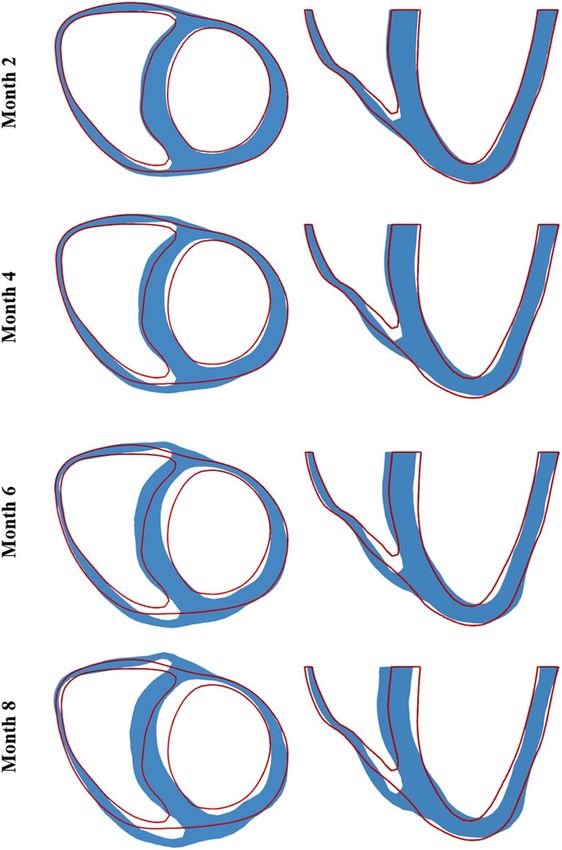
www.nature.com/scientificreports/                                                               www.nature.com/scientificreports

                           Figure 1. (a) Propagation of the depolarization isochrones in the Normal (top) and Pacing (bottom) cases. (b)
                           Long term changes in RV (left) and LV (right) PV loops in the Pacing case; M0–8 denote results at 0–8 month.
                           Refer to (c) for line color. (c) Fiber stretch λf as a function of time over a cardiac cycle at 0–8 month. Normal
                           case is in black.

                               Motivated by these experimental observations, we seek here to investigate if prescribing myofiber stretch as
                           a single stimulus that controls growth in the myofiber and transverse directions (with different sensitivity) can
                           quantitatively reproduce long term changes in ventricular geometry associated with mechanical dyssynchrony.
                           Based on a recently developed modeling framework8,16, we simulate anisotropic growth that is driven solely by
                           the local maximum elastic myofiber stretch. We seek to determine if it is possible to find different forward and
                           reverse growth rates in the longitudinal and transverse directions that can simultaneously and quantitatively
                           reproduce global and local asymmetrical changes in biventricular geometry associated with those found in pre-
                           vious chronic pacing experiments5,17. We show that with appropriate calibration of the growth rates, the coupled
                           electromechanics-growth model can reproduce changes in the biventricular geometry that are qualitatively com-
                           parable with previous experimental measurements and clinical observations5,17, suggesting that it is possible for
                           myofiber stretch to be the sole growth stimulant in mechanical dyssynchrony.

                           Results
                           We present short-term and long-term results of anisotropic growth and remodeling (G&R) constitutive model.
                           Details of the model and simulation cases are given in the Method section.

                           Activation patterns. Figure 1a shows the activation patterns for the Normal and Pacing cases. In the Normal
                           case, the depolarization isochrones propagated towards the left ventricular free wall (LVFW) and right ventricular
                           free wall (RVFW) upon septal initiation. The entire biventricular unit was activated at about 80 ms (approximately
                           the QRS duration). Conversely in the Pacing case, depolarization isochrones propagated from the LVFW towards
                           the septum and then the RVFW, resulting in a longer activation time of ∼120 ms for the entire biventricular unit.

                           Regional variation of myofiber stretch. Figure 1b shows the spatially-averaged elastic myofiber stretches
                           λf in the RVFW, septum, and LVFW for the Pacing and Normal cases taken with respect to the end-diastolic
                           configuration. In the Pacing case, pre-systolic myofiber stretch (i.e., λf > 1) was present only in the late-activated

Scientific Reports |   (2019) 9:12670 | https://doi.org/10.1038/s41598-019-48670-8                                                             2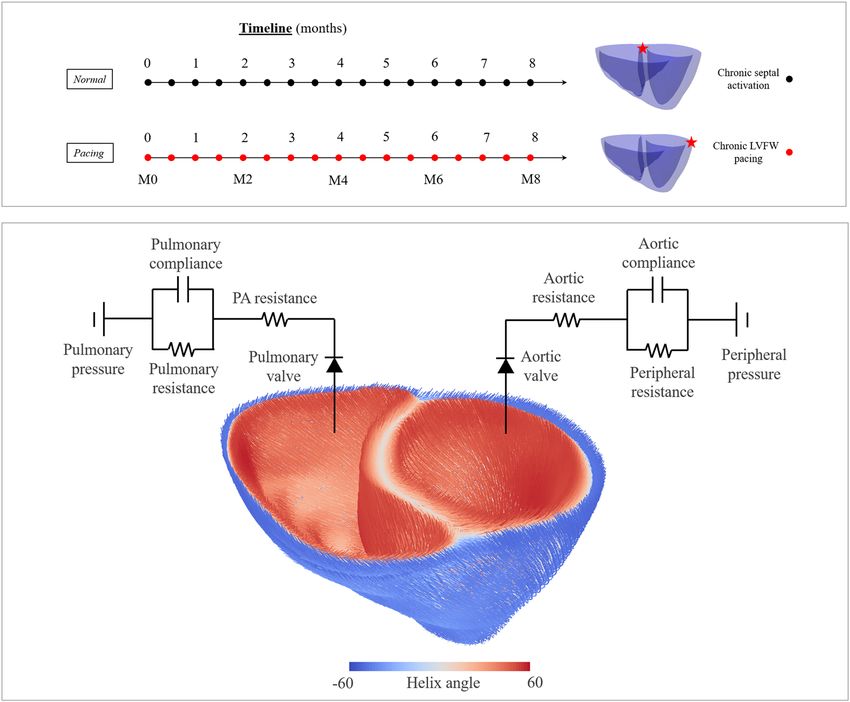
www.nature.com/scientificreports/                                                               www.nature.com/scientificreports

                           Figure 2. Long-term changes in biventricular geometry (blue) are superimposed on the original (red outline).
                           Left: short-axis view; Right: long-axis view.

                           RVFW and septum, with a higher value found in the latter. By contrast, only a small pre-systolic myofiber stretch
                           was found at the LVFW in the Normal case compared to that in the septum of the Pacing case. Consequently,
                           myofiber stretch in the septum + RVFW and LVFW of the Pacing case deviated positively and negatively from
                           the homeostatic value in the Normal case. This heterogeneity in myofiber stretch λf resulted in the evolution of
                           growth scalars θi’s towards θi,max in the late activated septum/RV, and θi,max in the early-activated LVFW, leading to
                           long-term asymmetrical geometrical changes.

                           Pressure-volume relationship. Figure 1c shows the long-term changes in the LV and right ventricle (RV)
                           pressure-volume (PV) loops for the Pacing case. There was no immediate substantial reduction in pump function
                           in the Pacing case (0 month). Changes were, however, noticeable at 2 months in the form of a progressive LV dila-
                           tion. Specifically, in the span of 8 months, LV end-diastolic volume (EDV) increased from 104.3 ml to 118.6 ml
                           whereas end-systolic volume (ESV) increased from 55.65 ml to 70.3 ml. This led to a rightward shift in the LV
                           PV loop that was accompanied by a slight change in ejection fraction (EF) from 48.7% to 48.3% in 8 months. On
                           the other hand, the simulations also show long-term changes of the RV PV loops due largely to thickening of the
                           septum. RV EDV slightly decreased from 104.9 ml to 103.7 ml whereas RV ESV increased from 53.6 ml to 57.1 ml
                           at 8 months.

                           Long-term local geometrical changes. Figure 2 shows the long-term changes in geometry of a short-axis
                           section taken at the mid-ventricular level and a long-axis section that are typically assessed in experimental
                           and clinical studies. As shown in the figure, long-term changes in the geometry is highly asymmetrical in the
                           biventricular unit in the Pacing case with radial wall thickening occurring at the late-activated septum and wall
                           thinning occurring at the early-activated LVFW. Shown quantitatively in Fig. 3, the model predicted a monotonic
                           increase in LV EDV (13.7%), septum wall volume (60.7%) and septum wall thickness (27.5%) over an 8 months
                           period. Conversely, RVFW and LVFW thickness decreased by (12.3%) and (20.4%) over the same period, respec-
                           tively. Wall volume of the LVFW and RVFW as well as RV EDV behaves non-monotonically and were roughly
                           unchanged after 8 months.

Scientific Reports |   (2019) 9:12670 | https://doi.org/10.1038/s41598-019-48670-8                                                             3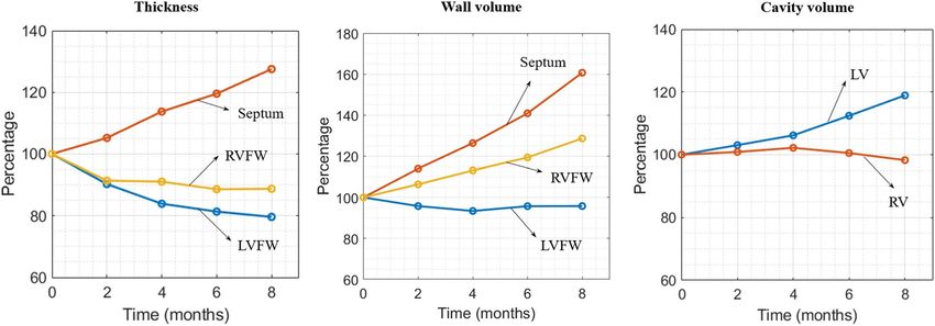
www.nature.com/scientificreports/                                                              www.nature.com/scientificreports

                           Figure 3. Long-term local geometrical changes. Left: wall thickness; Middle: wall volume; Right: Cavity
                           volume.

                           Discussion
                           Motivated by a recent experiment showing that longitudinal stretching of myocyte produces both longitudinal
                           and transverse growth via parallel and serial sarcomeric addition15, we have presented an anisotropic G&R consti-
                           tutive model in which the changes in lengths of the tissue in 3 orthogonal material directions are driven locally by
                           the deviation of maximum elastic myofiber stretch (over a cardiac cycle) from its corresponding homeostatic set
                           point value. This model is coupled to an electromechanics modeling framework to simulate the long-term effects
                           of asynchronous activation associated with LVFW pacing. We find that the application of elastic myofiber stretch
                           as the sole mechanical driver of G&R in the constitutive model can reproduce quantitatively both local and global
                           features of asymmetrical remodeling found in experiments of mechanical dyssynchrony as presented below.
                               In terms of acute behavior, our simulations show that in the presence of electromechanics alterations induced
                           by LVFW pacing, a pre-stretch occurs at the late activated regions (Septum + RVFW) in the beginning of systole
                           (Fig. 1) that resulted in a higher maximum elastic myofiber stretch compared to the homeostatic set point value
                           (during normal activation) found in those regions. The early activated region (LVFW), on the other hand, has
                           a lower maximum elastic myofiber stretch when compared to its corresponding homeostatic set point value.
                           These results are consistent with observations made in animal models of asynchronous activation18,19 and LBBB
                           patients20, where abnormal stretching of the tissue at the beginning of systole (i.e., pre-systolic stretching) were
                           found at the late activated regions.
                               Using the alteration of elastic myofiber stretch as a stimulant for G&R in all 3 material directions, the model
                           predictions, after appropriate calibration of parameters, are compared favorably to local and global measure-
                           ments in canine experiments with similar chronic LVFW pacing protocol5,17. A quantitative comparison of the
                           experimental results with model predictions are given in Table 1. In terms of local geometrical changes, the model
                           predicted an increase in septum wall thickness by 18.5% (cf. 23 ± 12% in the experiments5) and a decrease in
                           LVFW thickness by 19.7% (cf. 17 ± 17% in the experiments5) after 6 months of pacing. In terms of global geomet-
                           rical changes, the model predicts an increase in LV EDV by 9% (cf. 7.4 ± 29% in the experiments) and LVFW +
                           Septum wall volume by 9.5% (cf. 15 ± 17% in the experiments) for the same duration. As detailed in Table 1, the
                           chronic features of LVFW pacing predicted by the model are also found in LBBB21, which produces mechanical
                           dyssynchrony via an opposite activation pattern (i.e., septum is activated first followed by the LVFW).
                               Interestingly, our model also predicted that the RV wall thickness is changed in LVFW pacing in response
                           to the presence of a pre-systolic stretch (Fig. 1). Unfortunately, measurements of RVFW geometrical changes in
                           response to LVFW pacing are, to the best of our understanding, not available for comparison. While there are a
                           small number of studies on right branch bundle block (RBBB) which has similar (left to right) activation pattern
                           as in LVFW pacing, the presence of RBBB is either superimposed on tachypacing-induced heart failure22 or is
                           confounded by other diseases such as Tetralogy of Fallot23.
                               Our study shows that it is necessary to impose different forward growth rate τg and reverse growth rate τrg
                           in order to reproduce asymmetrical hypertrophy. Additional simulations using the same forward and reverse
                           growth rates produce excessive thickening in the septum compared to LVFW case and are not able to predict
                           the observed asymmetrical hypertrophy (See Appendix). While direct measurements of reverse growth rates on
                           isolated cardiomyocytes are, to the best of our knowledge, not available, large animal and clinical studies have
                           suggested that the reverse growth rates are likely to be different from the forward growth rates. For example, the
                           study by Vernooy et al.24 found that regional LV mass does not return to normal values (100%) during biventricu-
                           lar pacing. Similarly, the study by Gerdes et al.25 also suggests that cardiac hypertrophy induced by aortocaval
                           fistula in rats may not be completely reversible upon reversal of fistula.
                               As with most constitutive models describing cardiac G&R, the model described here is developed based on
                           the volumetric growth framework6 that largely focuses on changes in the morphology of the myocytes as they
                           undergo hypertrophy or atrophy (as opposed to turnover of extracellular matrix constituents) during G&R11.
                           One of the key differences between these G&R constitutive models is in the prescription of G&R stimuli in their
                           formulation. Goktepe9 et al. proposed using two different types of G&R stimuli, namely, elastic myofiber stretch

Scientific Reports |   (2019) 9:12670 | https://doi.org/10.1038/s41598-019-48670-8                                                           4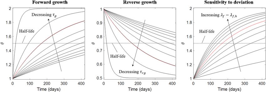
www.nature.com/scientificreports/                                                                     www.nature.com/scientificreports

                                                           LVFW pacing LVFW Pacing Experiment        LBBB Experiment          LVFW Pacing Experiment
                          Parameter                Month   Simulation  (Van Oosterhout et al., 1998) (Vernooy et al., 2004)   (Prinzen et al., 1995)
                                                   0       100           100 ± 27.8                   100 ± 29.8              100
                                                   2       102.3         —                            117.5 ± 12.8            —
                          LVEDV (% of Normal”)     4       104.6         —                            129.8 ± 50.9R           —
                                                   6       109           107.4 ± 29.9M                —                       —
                                                   8       113.7         —                            —                       —
                                                   0       48.7          35.3 ± 7.0                   43 ± 4                  100
                                                   2       48.3          —                            —                       —
                          LVEF (%)                 4       48.6          —                            33 ± 6R                 —
                                                   6       47.8          39.6 ± 8.9M                  —                       —
                                                   8       48.3          —                            —                       —
                                                   0       100           100                          —                       100
                                                   2       104.9         —                            —                       —
                          LVESV (% Change)         4       108.7         —                            —                       —
                                                   6       118.5         —                            —                       —
                                                   8       126.4         —                            —                       —
                                                   0       100L          100L                         100C                    100L
                                                   2       90.3L         90.7 ± 8.7L                  —                       88.9 ± 6.8L,R
                          Early activated region
                                                   4       83.9L         87.0 ± 7.2L                  —                       79.7 ± 8.0L,R,*
                          thickness (% change)
                                                   6       81.3L         86.5 ± 16.7L,R               —                       —
                                                   8       79.6L         —                            —                       —
                                                   0       100C          100C                         100L                    100C
                                                   2       105.2C        108.4 ± 11.3C                —                       96.8C,M
                          Late activated region
                                                   4       113.7   C
                                                                         110.5 ± 16.8  C
                                                                                                      —                       103.0 ± 7.5C,M,*
                          thickness (% Change)
                                                   6       119.6   C
                                                                         122.5 ± 11.3  C,R
                                                                                                      —                       —
                                                   8       127.5C        —                            —                       —
                                                   0       100           100                          100                     100
                                                   2       91.4          —                            —                       —
                          RV thickness (% Change) 4        91.1          —                            —                       —
                                                   6       88.6          —                            —                       —
                                                   8       88.7          —                            —                       —

                           Table 1. Comparison with experimental data5,17,21. Mdenotes no significant change over time; Rdenotes
                           significant change over time (p < 0.05). LDenotes LVFW Thickness; Cdenotes septum thickness. *Denotes 3
                           months; —denotes not reported or measured.

                           for driving growth in the myofiber direction and Mandel stress for driving growth in directions transverse to
                           the myofiber. They show that this formulation can reproduce features that are qualitatively in agreement with
                           eccentric and concentric hypertrophy (i.e., volume and pressure overload). It is not clear, however, if it can predict
                           asymmetrical remodeling features found in mechanical dyssynchrony. Subsequently, Kerckhoffs et al.10 proposed
                           using a single type of G&R stimuli, namely, strain in their model. While the G&R stimuli in the myofiber direc-
                           tion is similar to Goktepe et al.9 in their model, they proposed using normal strain components transverse to the
                           myofiber direction as stimuli for growth in the transverse directions. They showed that this formulation is able to
                           reproduce features associated with global remodeling in pressure and volume overload as well as local remodeling
                           associated with LBBB14. A detailed comparison of existing cardiac G&R constitutive models based on equibiax-
                           ial loading can be found in Witzenburg and Holmes26. In contrast to the G&R models described above, elastic
                           myofiber stretch is prescribed here as the driver for growth in both the myofiber and transverse directions, but
                           with different sensitivity (or rates). This assumption is consistent with a recent study that observed in real time
                           both longitudinal elongation and lateral extension occurring in the myocyte in response to longitudinal stretch-
                           ing15. With appropriate calibration, we show that the prescription of a single growth stimuli based only on elastic
                           myofiber stretch can quantitatively reproduce the largely local G&R features that are associated with mechanical
                           dyssynchrony, which reinforce the theory that transverse growth maybe controlled, at least to some extent, by
                           elastic myofiber stretch that previous models have not considered.
                               Although the anisotropic growth model predictions are generally consistent with experimental and clini-
                           cal measurements, the model presented here, nonetheless, could be further improved with time. First, we have
                           not considered sarcomeric parallel addition under lateral stretch as found in the experiment15 because changes
                           in myofiber (longitudinal) stretch is the most prominent asymmetrical feature of asynchronous activation.
                           Moreover, without any direct measurements of forward and reverse growth rates associated individually with
                           lateral and longitudinal stretch, it is difficult to separate parallel addition of sarcomere due to changes in lateral
                           stretch from that due to longitudinal stretch to reproduce clinically observed features of asynchronous activation.
                           Inclusion of lateral stretch as a growth stimuli in the model can be incorporated in future studies with the availa-
                           bility of more experimental data. Second, we did not consider any myocardial material property changes that may

Scientific Reports |   (2019) 9:12670 | https://doi.org/10.1038/s41598-019-48670-8                                                                     5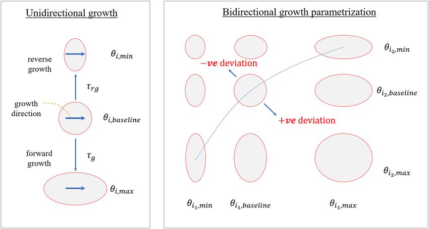
www.nature.com/scientificreports/ www.nature.com/scientificreports
occur during the remodeling process. This limitation is shared by growth models developed based purely on the
volumetric growth framework, which cannot directly accommodate for any changes in the mechanical properties.
Structural changes in the tissue such as the reorientation of the collagen fibers were also not considered in our
simulations. Nonetheless, the experiments did not report any change in the myocardial collagen fraction5, sug-
gesting that extracelluar matrix remodeling is limited in mechanical dyssynchrony. Third, we have also assumed
a constant preload and afterload in the entire simulation. Besides ventricular G&R, the circulatory system may
also adapt during the long-term27. Specifically, models reflecting improvements in ventricular-arterial coupling
during reverse remodeling28 are expected to better capture long-term changes in CRT. We also did not account
for any electrophysiological remodeling that may occur during electromechanics alterations. Besides changes in
geometry, the myocyte’s electrophysiological properties such as action potential duration29 may be altered during
the remodeling process. Last, our simulations did not consider the fact that asynchronous contraction can induce
mitral regurgitation (MR), which may in turn confound the G&R process by inducing volume overload. Evidence
that asynchronous contraction produces MR is supported by the observation that the severity of baseline MR
is decreased in CRT patients30,31 when their mechanical dyssynchrony is corrected. The model, which we have
shown is able to reproduce features associated with volume (and pressure) overload (See Appendix) using fiber
stretch as the growth stimuli, can be used in future studies to evaluate such possibilities.
In summary, we have presented an anisotropic growth model that simulates asymmetric growth in mechan-
ical dyssynchrony. We show that by using the maximum elastic fiber stretch as the sole growth stimulant, the
model can reproduce long-term features that agree quantitatively with the experimental and clinical findings. The
growth model may be useful for optimizing the long-term pacing effects of cardiac resynchronization therapy in
future studies.
Methods
Growth constitutive model. Here we let χκ (X , t ) describe the mapping from an unloaded (stress-free)
0
reference configuration κ0 with material point position X to a current configuration κ with the corresponding
material point position x = χκ (X , t ). The displacement field is given by u(X) = x − X and the deformation
0
∂χ
gradient tensor corresponding to the mapping is defined as F = κ0 . Under the volumetric growth framework6,
∂X
we multiplicatively decomposed the deformation gradient tensor, i.e.
F = FeFg , (1)
into an elastic component Fe and an incompatible growth component Fg. The growth deformation gradient Fg was
parameterized by the scalar growth multipliers θf, θs and θn in the following tensorial form
Fg = θf f0 ⊗ f0 + θs s 0 ⊗ s 0 + θn n 0 ⊗ n 0 , (2)
where f0, s0 and n0 are local myofiber, sheet, and sheet-normal directions in the reference configuration. The
evolution of the growth multipliers was described based on deviations of a prescribed stimulant sj from its home-
ostatic value si,h. Specifically, the evolution of growth multipliers was described by the following ordinary differ-
ential equation16.
θi = k i (θi , si )gi (si − si , h) for i = f , s, n, (3)
where ( ) is the derivative with respect to time t and ki (θi, si) are rate limiting functions that restrict forward and
.
reverse growth rates. The function gi (si− si,h) depends on local stimulus and we prescribed a simple linear form,
i.e., gi (si − si,h) = si − si,h. The rate limiting function was defined as follows
γg , i
1 θmax , i − θi
if gi (si − si , h) ≥ 0
τg , i θmax , i − θmin , i
k i (θi , si ) = ,
γrg , i
1 θi − θmin , i
if gi (si − si , h) < 0
τ θ − θmin , i
rg , i max , i
(4)
where the subscript i = f, s, n denote the association with the myofiber, sheet, and sheet-normal directions. The
growth constitutive model parameters τg,i, τrg,i, γg,i and γrg,i control the rates of growth and reverse growth, which
may be different. The main purpose of the rate-limiting function is to restrict the evolution of the growth multi-
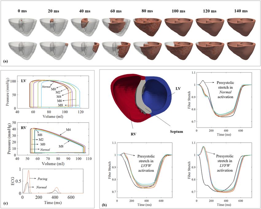
pliers θi to lie within some prescribed limits7 (Fig. 4). Allowing the rate limiting function ki (θI, s) to be prescribed
individually in each i direction enables a broad spectrum of anisotropic growth deformation to be produced.
Based on previous experimental findings15, maximum elastic myofiber stretch was prescribed as the growth
stimuli in all 3 material directions (i.e., si = λf for i = f, s, n). The myofiber stretch was defined by
λf = f0 . CEDf0 , (5)
where CED denotes the right Cauchy-Green deformation tensor with respect to the end-diastolic configuration
T
that was, in turn, defined by CED = FED FED with FED = Fe(Fr,ED)−1 and Fr,ED representing the map from the
unloaded configuration to the end-diastolic configuration. As depicted in Fig. 4, positive deviations from home-
ostatic stretch in the growth constitutive model will result in the growth multiplier θi evolving towards θmax,i,
Scientific Reports | (2019) 9:12670 | https://doi.org/10.1038/s41598-019-48670-8 6www.nature.com/scientificreports/ www.nature.com/scientificreports
Figure 4. Schematic of the anisotropic growth evolution in response to local stimulus.
which is typically an expanded configuration. Conversely, negative deviations from homeostatic stretch will result
in the growth multiplier θi evolving towards θmin,i, which is typically a shrunk configuration.
Electromechanics model. Cardiac electrophysiology. Cardiac electrical activity and its propagation was
modeled using the modified Fitzhugh-Nagumo and monodomain equations32. Specifically, the spatio-temporal
evolution of cardiac action potential φ was described in the reference configurations by
φ = div(D grad φ) + fφ (φ, r ) + Is , (6a)
r = fr (φ, r ), (6b)
where D = d isoI + danif0 ⊗ f0 is the anisotropic electrical conductivity tensor (with faster conduction along
myofiber direction), Is is the constant electrical stimulus for prescribing local excitation initiation and pacing or
both. Variables φ and r are dimensionless and r is a recovery variable. The excitation properties of cardiac tissue
were defined using:
fφ = cφ(φ − α)(1 − φ) − rφ, (7a)
fr = (γ + rγ (φ))( − r cφ(φ − b − 1)), (7b)
which is a modification of the Fitzhugh-Nagumo equations following Aliev and Panfilov with model param-
33,34 32
eters c, α, b, and γ. The function γ (φ) = μ1/(μ2 + φ) in Eq. (7b) allows for the tuning of cardiac restitution with
parameters μ1 andμ2.
Cardiac mechanics. An active stress formulation was used to describe the mechanical behavior of the cardiac
tissue. In this formulation, the cardiac tissue constitutive relation was prescribed separately for passive and active
mechanical behavior. Specifically, the second Piola-Kirchkoff or PK2 stress tensor S was additively decomposed
into a passive component Sp and an active componentSa, i.e.:
S = Sp + Sa. (8)
The tissue passive mechanical behavior was described using the following Fung-type strain energy function 35
based on the Green-Lagrange elastic strain tensor Ee:
C
W (Ee ) = (exp(Q) − 1),
2 (9)
where Q = bf E 2ff
+ (
bfs E 2fs
+ Esf2
+ + 2
E fn + Enf2 + ) + bxx (Ess2
+ 2
Ens2 Esn2 ) with
material parameters C, bf, bfs,
Enn
b xx, and E ij with (i,j) ∈ (f, s, n) denoting the components of the elastic Green-Lagrange strain tensor
1
Ee = 2 (FeTFe − 1) corresponding to the material coordinates. Incompressibility of the tissue was enforced by an
augmented strain energy function
Scientific Reports | (2019) 9:12670 | https://doi.org/10.1038/s41598-019-48670-8 7www.nature.com/scientificreports/ www.nature.com/scientificreports
ˆ (E , p) = W (E ) − p(J − 1),
W (10)
e e
where p is a Lagrange multiplier for enforcing the kinematic constraint J = det Fe = 1. The stress tensor was
derived from the augmented strain energy function by
ˆ (E , p)
∂W e
Sp = .
∂Ee (11)
A phenomenological active contraction model was used to describe contraction of the tissue upon excitation.
In this model, the active (fiber-directed) stress tensor was defined by:
Sa = T (t , tinit(X ), Ca0, E ff , Tmax )f0 ⊗ f0 . (12)
Magnitude of active force T was defined by a sarcomere length-dependent contractile force generation
model36,37:
Ca20 ((
1 − cos ω t , tinit , E ff ))
(
T t , tinit(X ), Ca0, E ff , Tmax = Tmax ) ( )
1 + ECa250 E ff 2 (13)
where Ca0 is the peak intracellular calcium concentration, Tmax is a scaling factor for the tissue contractility, and
ECa50 is the length-dependent calcium sensitivity given by:
(Ca0)max
ECa50 =
exp(B(l − l 0)) − 1 (14)
with material constant B, prescribed maximum peak intracellular calcium concentration (Ca0)max, instantane-
ous sarcomere length l, and sarcomere length at which no active tension develops l0. The instantaneous sarcomere
length was defined based on the prescribed initial length of sarcomerel s0, and was calculated using
l = ls 0 f0 . Cef0 .
Coupling electrophysiology and mechanics. The active contraction model was modified to incorporate
a spatially heterogeneous activation initiation time tinit(X) that accounts for asynchronous depolarization based
on the action potential φ. The function ω in Eq. (13) is given by:
t
π sa if 0 ≤ tsa < t0
t0
ω=
π tsa − t0 + tr if t ≤ t < t + t
0 sa 0 r
tr
0
if t0 ≤ tsa < t0 + tr (15)
that explicitly defines active contraction based on time since activation tsa (X) = tcurrent− tinit (X), with tcurrent
denoting the current time in the cardiac cycle as:
tinit(X ) = inf{ t(X )|φ(X , t ) ≥ 0.9} (16)
defining the local initiation time that couples cardiac electrophysiology and mechanics. In Eq. (15), t0 is the pre-
scribed time to maximum active tension and tr is the sarcomere length-dependent active tension relaxation time
that is given by tr = ml + b with parameters m and b.
Computational approximation. Discretizing time using an implicit backward Euler scheme, approximate
solutions of the weak formulation for the acute electromechanics problem were obtained using the finite element
(FE) method, where we seek to find u ∈ H1(Ω), p ∈ L2(Ω), PLV ∈ , PRV ∈ , c1 ∈ 3, c2 ∈ 3, ϕ ∈ H1(Ω), r ∈ H0(Ω),
such that the below equations:
−T
δ = ∫Ω (FS − JF ): grad δu dV − ∫Ω δp(J − 1)dV
−PLV ∫ JF −T : grad δu dV − PRV ∫ JF −T : grad δu dV
Ω LV , cav Ω RV , cav
−δPLV (VLV , cav(u ) − VLV , p) − δPRV (VRV , cav(u )VRV , p)
−δc1. ∫ udV − δc2. ∫ X × u dV − c1. ∫ δudV − c2. ∫ X × δudV
Ω Ω Ω Ω
−∫ kspring 1u . δudS − ∫ kspring 2u . δudS = 0
∂Ω epi ∂Ω b (17a)
−1
∫Ω (φ − φn)Δt δφ = ∫Ω D grad φ. grad δφ + ∫Ω (fφ + Is ) δφ (17b)
Scientific Reports | (2019) 9:12670 | https://doi.org/10.1038/s41598-019-48670-8 8www.nature.com/scientificreports/ www.nature.com/scientificreports
∫Ω (r − rn)Δt−1δr = ∫Ω fr δφ (17c)
3 3
are satisfied for all test functions δu ∈ H (Ω), δp ∈ L (Ω), δPLV ∈ , δPRV ∈ , δc1 ∈ , δc2 ∈ , δϕ ∈ H1(Ω),
1 2
δr ∈ H0(Ω). Domains ΩLV,cav and ΩRV,cav denote LV and RV cavities, respectively. Spring constants kspring1 and kspring2
model are associated with the robin-type boundary conditions imposed at the epicardial surface ∂Ωepi and basal
surface ∂Ωb, respectively. Variables c1 and c2 are Lagrange multipliers38 to constrain rigid body translation and
rotation, respectively. Variables PLV and PRV are Lagrange multipliers39 constraining the LV and RV cavity volumes
to their corresponding prescribed values VLV,p and VRV,p, respectively. Cavity volumes VLV,cav (u) and VRV,cav (u) were
estimated using the divergence theorem39. It can be shown that the computed Lagrange multipliers PLV and PRV
are equivalent to the LV and RV cavity pressures, respectively. Note that PLV and PRV are different from the
Lagrange multiplier p which is a scalar field, i.e., p = p(C, t) to enforce local incompressibility and depends on the
spatial location of the myocardium.
We used a Galerkin FE discretization with piecewise quadratic element for the spatial approximation of dis-
placements u(X), continuous piecewise linear elements for hydrostatic pressure p and action potential φ. We
used discontinuous Galerkin elements to approximate the recovery state variable r and fiber stretch λf. A realistic
human biventricular geometry, that was reconstructed from magnetic resonance images from a previous study40,
was used for the computational study. Helix angle defining the myofiber direction f0 was prescribed to vary line-
arly across the myocardial wall from 60° at the endocardium to −60° at the epicardium using a Laplace-Dirichlet
rule-based algorithm41. Fiber directions f0 as well as the orthogonal sheet direction s0 and sheet-normal direction
n0 were prescribed at the quadrature points. A FE mesh with 11988 tetrahedral elements was used to discretize the
biventricular geometry and FEniCS42 was used for computational implementation. The time interval (0, T) was
discretized into subintervals[tn, tn + 1], n = 0, 1, …, with tn = nΔt and Δt denoting a fixed time step.
Simulating the full cardiac cycle. Complete cardiac cycles with each having a duration of 750 ms were simulated
using the electromechanics model. Specifically, passive filling was simulated by incrementally applying pressure
to the LV and RV endocardial surfaces until their prescribed EDV was reached. Thereafter, systole was simulated
by applying a current to different locations in the biventricular unit depending on the pacing protocol. The LV
and RV cavity volumes were constrained to remain constant during the isovolumic contraction phase, which
terminated when the LV and RV cavity pressures exceeded the prescribed aortic and pulmonary artery pressures,
respectively. The subsequent ejection phase was simulated by coupling the LV and RV cavity volumes each to
a 3-element Windkessel model (Fig. 5). Ejection phase in each cavity was terminated when the cavity outflow
rate became less than 0.005 ml/min. The cavity volumes were then prescribed to remain constant to describe the
isovolumic relaxation phase. The isovolumic relaxation phase was terminated based on prescribed pressures for
initiation of diastolic filling, which was then passively prescribed until end of diastole.
Separation of time scale between growth and elastic deformation. To integrate growth with the
electromechanics model, we adopted a similar approach to separate the time scale as described in Lee et al.8.
Specifically, since appreciable G&R can only be observed after large number of heartbeats, the growth tensor
Fg was treated as a constant that is independent of time in the electromechanics model and updated after each
cardiac cycle. Approximate solutions of the weak formulation for the G&R problem were obtained using the FE
method where we seek to find u ∈ H1(Ω), p ∈ L2(Ω), such that the below equation
−T
δ G = ∫Ω (FS − JF ): grad δu dV − ∫Ω δp(J − 1)dV
−∫ kspring1u . δudS = 0,
∂Ω epi (18)
is satisfied for all test functions for all δu ∈ H (Ω) and δp ∈ L (Ω). The above equation describing the
1 2
long-term evolution differs from the Eq. (17) describing short-term evolution in the following ways: there is no
active stress in the long-term model; and the short-term model was solved for cavity pressures with prescribed
volumes while the long-term model is solved for cavity volumes at prescribed (zero) cavity pressures. We used a
Galerkin FE discretization with piecewise quadratic FE for the spatial approximation of displacements u(X). We
used discontinuous Galerkin elements to approximate the growth parameters θis. The algorithm used to update
the geometry (long-term problem) is described follows:
• Obtain maximum elastic stretch λf by solving the short time-scale problem over a cardiac cycle using Eq. (17)
• Initialize θi1s from the latest geometry
• Use λf,h from baseline model to estimate (λf − λf,h)
• For j = 1 to ngrowthSteps
• ( )
Explicitly update growth parameters: θi j +1 = θi j + k i θi j , λ f (λ f − λ f , h)
• Update Fg using θi j +1
• Solve for new geometry using Eq. (18).
Similar to our previous approach8, residual stresses induced by the incompatible growth tensor were removed
after each growth cycle. As a consequence of this F = Fe in Eq. (17a).
Scientific Reports | (2019) 9:12670 | https://doi.org/10.1038/s41598-019-48670-8 9www.nature.com/scientificreports/ www.nature.com/scientificreports
Figure 5. Top: Simulated chronic pacing timelines are shown. Pacing locations are indicated in the geometry
using a red star. Bottom: Myofiber architecture and lumped circulation model.
Growth parameters
τg τg γ θmin θ0 θmax
(no (no (no
Direction Days Days Days units) units) units)
θf 3.8 9.6 1.0 0.5 1.0 2.0
θs 9.6 3.8 1.0 0.5 1.0 2.0
θn 9.6 3.8 1.0 0.5 1.0 2.0
Table 2. Model parameters.
Simulation cases. Two cases differing in terms of the prescribed activation initiation location were simu-
lated. These cases are, namely,
• Normal: activation was initiated at the septum near the base,
• Pacing: activation was initiated at the LVFW near the base.
A schematic of the simulation timeline and pacing location is shown in Fig. 5. The homeostatic set point for
the maximum elastic myofiber stretch si,h = λf,h in the growth constitutive model in Eq. (3) was prescribed using
the local values obtained from the “Normal” case with septal activation. Deviations of the maximum elastic fiber
stretch in the “Pacing” case from the homeostatic values were used as growth stimuli.
Calibration of G&R simulations. Growth parameters used in the simulations are shown in Table 2. All
other model parameters are given in the Appendix. Based on Eqs (3) and (4), half-life is given by
θmax − θmin
t 1 , j = τj ln(2) ,
2 λ f − λ f ,h (19)
with subscript j = g,rg and γg,i = γrg,i = 1.0. Using a deviation of λf − λf,h = ±0.06, τg and τrg were initialized with
a half-life of 170 days for θs and θn. Given the exponential decay, this will produce an increase in θs and θn by 53%
Scientific Reports | (2019) 9:12670 | https://doi.org/10.1038/s41598-019-48670-8 10www.nature.com/scientificreports/ www.nature.com/scientificreports
Figure 6. Effect of varying G&R parameters. Changes in Left: τg from 40.0 to 1.0 for λf − λf,h = 0.06; Middle:
τg from 40.0 to 1.0 for λf − λf,h = −0.06; Right: λf − λf,h from 0.01 to 0.1 for τg = 9.6. Red: Parameter values in
Table 2.
in 6 months. The net change in thickness also depends on the material properties of the body prescribed during
growth deformations8 and hence, the simulated changes in wall thickness were expected to be lesser. Forward
growth rates for θf and reverse growth rates for θs and θn were adjusted together to match LV dilation and early
activated region thinning, respectively. The sensitivity of growth rates to λf − λf,h = ±0.06 is shown in Fig. 6. In
six months, a change in λf − λf,h from 0.06 to 0.08 would result in corresponding changes in θs and θn from 53%
to 63%.
References
1. Prinzen, F. W., Augustijn, C. H., Arts, T., Allessie, M. A. & Reneman, R. S. Redistribution of myocardial fiber strain and blood flow
by asynchronous activation. Am. J. Physiol. Circ. Physiol. 259, H300–H308 (1990).
2. Fahy, G. J. et al. Natural history of isolated bundle branch block. Am. J. Cardiol. 77, 1185–1190 (1996).
3. Eriksson, P., Wilhelmsen, L. & Rosengren, A. Bundle-branch block in middle-aged men: risk of complications and death over 28
yearsThe Primary Prevention Study in Göteborg, Sweden. Eur. Heart J. 26, 2300–2306 (2005).
4. Schneider, J. F. et al. Comparative features of newly acquired left and right bundle branch block in the general population: the
Framingham study. Am. J. Cardiol. 47, 931–40 (1981).
5. van Oosterhout, M. F. M. et al. Asynchronous Electrical Activation Induces Asymmetrical Hypertrophy of the Left Ventricular Wall.
Circulation 98, 588–595 (1998).
6. Rodriguez, E. K., Hoger, A. & McCulloch, A. D. Stress-dependent finite growth in soft elastic tissues. J. Biomech. 27, 455–467 (1994).
7. Lubarda, V. A. & Hoger, A. On the mechanics of solids with a growing mass. Int. J. Solids Struct. 39, 4627–4664 (2002).
8. Lee, L. C., Sundnes, J., Genet, M., Wenk, J. F. & Wall, S. T. An integrated electromechanical-growth heart model for simulating
cardiac therapies. Biomech. Model. Mechanobiol. 15, 791–803 (2016).
9. Göktepe, S., Abilez, O. J., Parker, K. K. & Kuhl, E. A multiscale model for eccentric and concentric cardiac growth through
sarcomerogenesis. J. Theor. Biol. 265, 433–442 (2010).
10. Kerckhoffs, R. C. P., Omens, J. H. & McCulloch, A. D. A single strain-based growth law predicts concentric and eccentric cardiac
growth during pressure and volume overload. Mech. Res. Commun. 42, 40–50 (2012).
11. Lee, L. C., Kassab, G. S. & Guccione, J. M. Mathematical modeling of cardiac growth and remodeling. Wiley Interdiscip. Rev. Syst.
Biol. Med. 8, 211–226 (2016).
12. Kroon, W., Delhaas, T., Arts, T. & Bovendeerd, P. Computational modeling of volumetric soft tissue growth: application to the
cardiac left ventricle. Biomech. Model. Mechanobiol. 8, 301–309 (2009).
13. Klepach, D. et al. Growth and remodeling of the left ventricle: A case study of myocardial infarction and surgical ventricular
restoration. Mech. Res. Commun. 42, 134–141 (2012).
14. Kerckhoffs, R. C. P., Omens, J. H. & McCulloch, A. D. Mechanical discoordination increases continuously after the onset of left
bundle branch block despite constant electrical dyssynchrony in a computational model of cardiac electromechanics and growth. EP
Eur. 14, v65–v72 (2012).
15. Yang, H. et al. Dynamic Myofibrillar Remodeling in Live Cardiomyocytes under Static Stretch. Sci. Rep. 6, 20674 (2016).
16. Lee, L. C. et al. A computational model that predicts reverse growth in response to mechanical unloading. Biomech. Model.
Mechanobiol. 14, 217–229 (2015).
17. Prinzen, F. W. et al. Asymmetric thickness of the left ventricular wall resulting from asynchronous electric activation: A study in
dogs with ventricular pacing and in patients with left bundle branch block. Am. Heart J. 130, 1045–1053 (1995).
18. McVeigh, E. R. et al. Imaging asynchronous mechanical activation of the paced heart with tagged MRI. Magn. Reson. Med. 39,
507–513 (1998).
19. Prinzen, F. W., Hunter, W. C., Wyman, B. T. & McVeigh, E. R. Mapping of regional myocardial strain and work during ventricular
pacing: Experimental study using magnetic resonance imaging tagging. J. Am. Coll. Cardiol. 33, 1735–1742 (1999).
20. Breithardt, O.-A. et al. Cardiac resynchronization therapy can reverse abnormal myocardial strain distribution in patients with heart
failure and left bundle branch block. J. Am. Coll. Cardiol. 42, 486 LP–494 (2003).
21. Vernooy, K. et al. Left bundle branch block induces ventricular remodelling and functional septal hypoperfusion. Eur. Heart J. 26,
91–98 (2005).
22. Byrne, M. J. et al. Diminished Left Ventricular Dyssynchrony and Impact of Resynchronization in Failing Hearts With Right Versus
Left Bundle Branch Block. J. Am. Coll. Cardiol. 50, 1484 LP–1490 (2007).
23. Marterer, R., Hongchun, Z., Tschauner, S., Koestenberger, M. & Sorantin, E. Cardiac MRI assessment of right ventricular function:
impact of right bundle branch block on the evaluation of cardiac performance parameters. Eur. Radiol. 25, 3528–3535 (2015).
24. Vernooy, K. et al. Cardiac resynchronization therapy cures dyssynchronopathy in canine left bundle-branch block hearts. Eur. Heart
J. 28, 2148–2155 (2007).
Scientific Reports | (2019) 9:12670 | https://doi.org/10.1038/s41598-019-48670-8 11www.nature.com/scientificreports/ www.nature.com/scientificreports
25. Gerdes, A. M., Clark, L. C. & Capasso, J. M. Regression of cardiac hypertrophy after closing an aortocaval fistula in rats. Am. J.
Physiol. 268, H2345–51 (1995).
26. Witzenburg, C. M. & Holmes, J. W. A Comparison of Phenomenologic Growth Laws for Myocardial Hypertrophy. J. Elast, https://
doi.org/10.1007/s10659-017-9631-8 (2017).
27. Arts, T., Delhaas, T., Bovendeerd, P., Verbeek, X. & Prinzen, F. W. Adaptation to mechanical load determines shape and properties
of heart and circulation: the CircAdapt model. Am. J. Physiol. Circ. Physiol. 288, H1943–H1954 (2005).
28. Paul, S. et al. Hemodynamic Effects of Long-Term Cardiac Resynchronization Therapy. Circulation 113, 1295–1304 (2006).
29. Spragg, D. D. et al. Abnormal conduction and repolarization in late-activated myocardium of dyssynchronously contracting hearts.
Cardiovasc. Res. 67, 77–86 (2005).
30. Breithardt, O. A. et al. Acute effects of cardiac resynchronization therapy on functional mitral regurgitation in advanced systolic
heart failure. J. Am. Coll. Cardiol. 41, 765 LP–770 (2003).
31. Ypenburg, C. et al. Acute Effects of Initiation and Withdrawal of Cardiac Resynchronization Therapy on Papillary Muscle
Dyssynchrony and Mitral Regurgitation. J. Am. Coll. Cardiol. 50, 2071 LP–2077 (2007).
32. Aliev, R. R. & Panfilov, A. V. A simple two-variable model of cardiac excitation. Chaos, Solitons & Fractals 7, 293–301 (1996).
33. FitzHugh, R. Impulses and physiological states in theoretical models of nerve membrane. Biophys. J. 1, 445–466 (1961).
34. Nagumo, J., Arimoto, S. & Yoshizawa, S. An active pulse transmission line simulating nerve axon. Proc. IRE 50, 2061–2070 (1962).
35. Guccione, J. M., McCulloch, A. D. & Waldman, L. K. Passive Material Properties of Intact Ventricular Myocardium Determined
From a Cylindrical Model. J. Biomech. Eng. 113, 42–55 (1991).
36. Guccione, J. M. & McCulloch, A. D. Mechanics of Active Contraction in Cardiac Muscle: Part I—Constitutive Relations for Fiber
Stress That Describe Deactivation. J. Biomech. Eng. 115, 72–81 (1993).
37. Guccione, J. M., Waldman, L. K. & McCulloch, A. D. Mechanics of Active Contraction in Cardiac Muscle: Part II—Cylindrical
Models of the Systolic Left Ventricle. J. Biomech. Eng. 115, 82–90 (1993).
38. Pezzuto, S., Ambrosi, D. & Quarteroni, A. An orthotropic active–strain model for the myocardium mechanics and its numerical
approximation. Eur. J. Mech. 48, 83–96 (2014).
39. Pezzuto, S. & Ambrosi, D. Active contraction of the cardiac ventricle and distortion of the microstructural architecture. Int. j. numer.
method. biomed. eng. 30, 1578–1596 (2014).
40. Henrik, F. et al. Efficient estimation of personalized biventricular mechanical function employing gradient‐based optimization. Int.
j. numer. method. biomed. eng. 0, e2982 (2018).
41. Bayer, J. D., Blake, R. C., Plank, G. & Trayanova, N. A. A Novel Rule-Based Algorithm for Assigning Myocardial Fiber Orientation
to Computational Heart Models. Ann. Biomed. Eng. 40, 2243–2254 (2012).
42. Logg, A., Mardal, K.-A. & Wells, G. Automated solution of differential equations by the finite element method: The FEniCS book. 84,
(Springer Science & Business Media, 2012).
Acknowledgements
This work was supported by NIH (R01 HL134841, U01 HL133359-01A1), NSF 1702987, AHA 17SDG33370110,
Burroughs Wellcome Fund.
Author Contributions
J.A. contributed to conception and design of the study; acquisition/analysis/interpretation of data; drafting/
revising the manuscript. J.M. contributed to acquisition/analysis/interpretation of data; drafting/revising the
manuscript. G.K. contributed to drafting/critical revision of the manuscript. L.C. contributed to conception and
design of the study; acquisition/analysis/interpretation of data; drafting/revising the manuscript.
Additional Information
Supplementary information accompanies this paper at https://doi.org/10.1038/s41598-019-48670-8.
Competing Interests: The authors declare no competing interests.
Publisher’s note: Springer Nature remains neutral with regard to jurisdictional claims in published maps and
institutional affiliations.
Open Access This article is licensed under a Creative Commons Attribution 4.0 International
License, which permits use, sharing, adaptation, distribution and reproduction in any medium or
format, as long as you give appropriate credit to the original author(s) and the source, provide a link to the Cre-
ative Commons license, and indicate if changes were made. The images or other third party material in this
article are included in the article’s Creative Commons license, unless indicated otherwise in a credit line to the
material. If material is not included in the article’s Creative Commons license and your intended use is not per-
mitted by statutory regulation or exceeds the permitted use, you will need to obtain permission directly from the
copyright holder. To view a copy of this license, visit http://creativecommons.org/licenses/by/4.0/.
© The Author(s) 2019
Scientific Reports | (2019) 9:12670 | https://doi.org/10.1038/s41598-019-48670-8 12You can also read