Human influence on growing period frosts like the early april 2021 in Central France
←
→
Page content transcription
If your browser does not render page correctly, please read the page content below
Human influence on growing period frosts like the
early april 2021 in Central France
Authors: R. Vautard (1), G. J. van Oldenborgh (2), R. Bonnet (1), S. Li (3), Y. Robin (4), S.
Kew (2), S. Philip (2), J.-M. Soubeyroux (4), B. Dubuisson (4), N. Viovy (5), M. Reichstein (6),
F. Otto (3)

(1) Institut Pierre-Simon Laplace, CNRS, Sorbonne Université, Université de Versailles - Saint
Quentin en Yvelines; (2) Koninklijk Nederlands Meteorologisch Instituut (3); University of
Oxford; (4) Météo-France; (5) Institut Pierre-Simon Laplace, CNRS, Commissariat à l’Energie
Atomique et aux énergies alternatives; (6) Max-Planck Institute für Biogeochemistry

Key results:

   ●   In early April 2021 several days of severe frost affected central Europe following an
       anomalously warm March. This led to very severe damages in grapevine and fruit
       trees, particularly in France, where young leaves had already unfolded in the warm
       early spring;

   ●   We analysed how human-induced climate change affected the temperatures as
       extreme as observed in spring 2021 over central France, where many vineyards are
       located. Analysing observations and 132 climate model simulations we found that
       without human-caused climate change, such temperatures in April would have been
       even lower by 1.2°C [0.7°C;1.6°C], compared to preindustrial conditions;

   ●   However, observed human-caused warming also affected the earlier occurrence of
       bud burst, characterized here by a growing-degree-day index value. This observed
       effect is stronger than the decrease in spring cold spells, thus exposing young leaves
       to more winter-like conditions with lower minimum temperatures and longer nights.
       The intensity of extreme frosts occurring after the start of the growing season such as
       those of April 2021 has increased by about -2°C, with a large range of uncertainty [-
       3.3°C to -0.6°C];

   ●   This observed intensification of growing-period frosts is attributable, at least in part, to
       human-caused climate change with each of the 4 large climate model ensembles
       (including a total of 132 model simulations) used here simulate a cooling of growing-
       period annual temperature minima of 0.5°C [0°C to 1°C] since pre-industrial, making
       the 2021 event 60% more likely [20%-120%];

   ●   Models accurately simulate the observed decreasing intensity in the lowest spring
       temperatures, but underestimate the observed trends in growing-period frost
       intensities;

   ●   Models all simulate a further intensification of frosts occurring in the growing period for
       future decades. The probability of an exceptional growing-period frost event such as
       that of 2021 (with a return period of 9 years in the current climate) is found to increase
       significantly by about 40% [20%-60%] in a climate with global warming of 2°C relative
       to pre-industrial.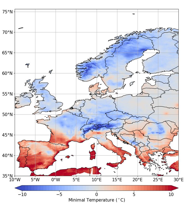
1. Introduction
Frost days and cold spells are decreasing in frequency in the northern latitudes (IPCC, 2014;
van Oldenborgh et al., 2019). Yet, severe cold spells continue to pound many mid-latitude
areas, due to the occasional occurrence of polar air being transported well into lower latitudes
as a consequence of the chaotic motion of Rossby waves. When occurring in spring, the
invasion of polar air into central and Southern Europe can create devastating frosts such as
happened in early April 2021. In such cases, when young leaves and flowers have started to
develop in fruit trees or grapevines, frost leads to massive damage in agriculture.
The 2021 frost event which took place from 6 to 8 April was exceptional with daily minimum
temperatures below -5°C were recorded in several places, leaving no chance to save
grapevines and fruit trees by frost management strategies (e.g as local heating from
braseros) in many places. The cold temperatures led to broken records at many weather
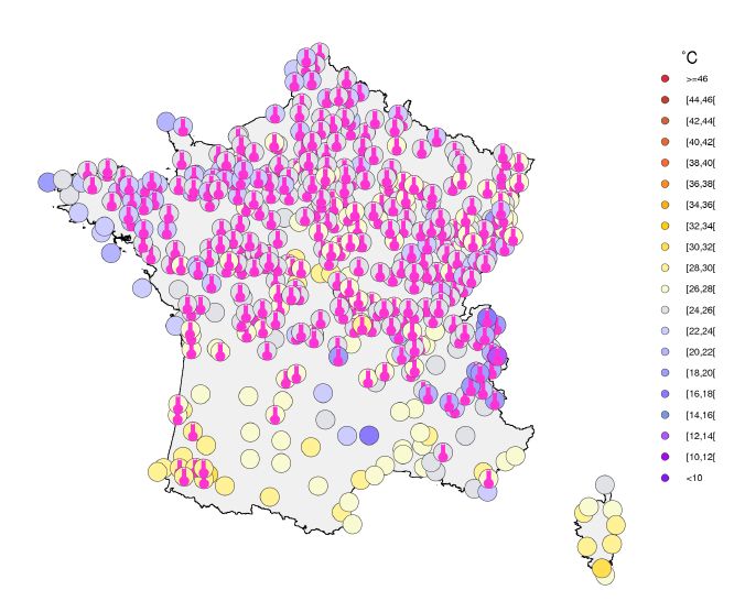
stations (see Figure 1, right-hand-side). Unfortunately, this cold event happened a week after
an episode of record-breaking high March temperatures also in many places in France and
Western Europe (Figure 1, left-hand-side). This sequence led the growing season to start
early, with bud burst occurring in March and the new leaves and flowers left exposed to the
deep frost episode that followed.
Figure 1: Stations with March (left) high records broken and April (right) low
records broken in 2021 (since at least 20 years) in France.
The frost impacts were widely covered by the French national media. According to the French
Ministry of Agriculture, “several hundreds of thousands of hectares were affected” and it was
assumed to be “probably the biggest agricultural disaster in the beginning of the 21st century”1.
According to the National Federation of Farmers' Unions (FNSEA), a third of the country’s
wine production could be lost and the combined losses in wine production and the
arboriculture sectors would amount to more than 4 billion euros2. In the Rhône region, farmers
estimated that the cold spell may have destroyed more than 80% of their harvests, affecting
1
https://www.lexpress.fr/actualites/1/societe/gel-la-plus-grande-catastrophe-agronomique-
du-siecle_2148731.html
2
https://www.reuters.com/article/us-france-wine-frost-idUSKBN2C915L ,
https://www.leparisien.fr/economie/gel-plus-de-4-milliards-deuros-de-pertes-estimees-dans-la-
viticulture-et-larboriculture-15-04-2021-24ZD6LV3V5A4LAH2UBCJ6RSVUA.php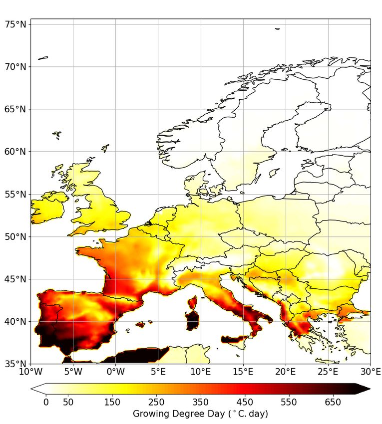
wines such as Côte-Rôtie, Côtes du Rhône and Condrieu. In Burgundy, “at least 50%” of the
harvests were reportedly lost, with the prestigious Chablis AOC especially hard hit3 .

The occurrence of such an event called for investigating the role of climate change. The cold
outbreak occurred with a specific weather pattern called the “Greenland Blocking”, identified
as one of the 4 main flow patterns that occur most frequently or are most stationary (Vautard
et al., 1990; Michelangeli et al., 1995). The combination of polar air advection, cloud-free sky
and still long nights led to hours of intense frost. Such dynamical events are not observed to
have become more frequent (Screen et al., 2013) despite the ongoing debate on the role of
narrower sea ice extent favoring the occurrence of blocking anticyclones (Barnes and Screen,
2015). The trend in circulation in April is the same as in winter, an intensification of westerly
flows that is not related to the weather observed in 2021 (not shown). However, the influence
of climate change on the evolution of daily minimum and maximum temperatures in a transition
month such as April could be significant, especially for agriculture when it comes to threshold
crossings.

The exceptional nature of the warm period preceding the 2021 event led to advancing
phenology. Recent studies show that despite the regression of frost days, the advance in the
start of the growing season has increased the number of frost days occurring in the growing
season in several places worldwide, including in Europe (Liu et al., 2018). Using several
indices for grapevine exposure, it has been found that the date of the latest frost day has not
regressed as fast as the date of growing season start (Sgubin et al., 2018). So far however no
formal attribution study of a “growing period frost” has been carried out quantifying the role of
anthropogenic climate change in these observed trends.. This article is devoted to an
attribution study of the “growing period frost” event witnessed in April 2021. It uses several
indices characterizing cold temperatures in the growing season. It also uses the well-
established attribution methodology described in Philip et al. (2020) and van Oldenborgh et
al. (2021).

In section 2, the indices chosen for the event definition are introduced. In Section 3, trends in
observations are analysed, and in section 4, trends in 5 model ensembles are analysed. In
Section 5 a conclusion and discussion are proposed.

2. Event definition and indices used
Despite the extent of the frost event that occurred between 6 and 8 April and the subsequent
damages, we focus here on central/northern France in order to investigate a relatively
homogeneous, mostly plain or low-elevation area. The area of concern, represented in Figure
2b encompasses [-1°- 5°E; 46°-49°N]. It covers most of the grapevine agriculture areas of
Champagne, Loire Valley and Burgundy which were identified as specifically vulnerable
regions under climate change (Sgubin et al., 2018). The area also covers regions with high
crop and fruit production. The area is represented in Figure 2b.

3
  https://www.liberation.fr/environnement/agriculture/pertes-liees-au-gel-les-agriculteurs-commencent-
a-sortir-leur-ardoise-20210416_HTV23WV4ABH4NGSDI5HN7NAKI4/
a) b) c)
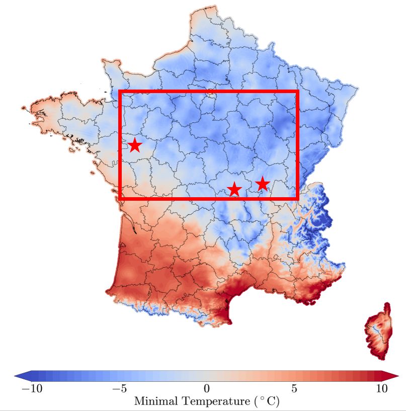
Figure 2. a) Minimum temperatures on 6 April 2021 in Europe from the E-OBS
database (see Section 3); b) focus on France with a higher resolution dataset,
using the Anastasia data (Météo-France, Besson et al, 2019). The study area is
shown in this panel by the bounded box in red; stars indicate the location of the 3
stations used to assess local trends; c) Spatial distribution of the Growing Degree
Day index in Europe on 5 April 2021 as calculated from E-OBS.
In order to examine the robustness of the assessment to the event definition several event
definitions are used, accounting for some phenological aspects. In each case, the “event” is
defined as the yearly minimum temperature (TNn) obtained under specific conditions, and
then averaged over the area, or taken at station locations. A basic reference conditioning is
the fixed-season minimum temperature: the TNn is calculated over the April-July months
(TNnApr-Jul). The second index accounts for phenology. The TNn is calculated conditioned
to the Growing Degree Day above 5°C (GDD) being larger than thresholds characterizing bud
burst conditions, which depend on species. In this study, our aim is not to tie thresholds to
specific plants' phenology but to provide a general overview for different thresholds. GDD is
calculated with a starting date of the previous winter solstice as in Garcia de Cortazar-Atauri
et al. (2009), which gives the formula for the GDD at day t during year y as:
with TM the daily mean temperature. In 2021, the values of GDD obtained on the day before
the frost events in the concerned area vary in the range 150°C.day to 350°C.day, with an
average value on 5 April of 259°C.day. This value is high for this calendar day (rank=14th
since 1921) but the record value was obtained in 2020, with a mean GDD of 320°C.day. Given
the range of values taken in the domain, we considered 3 thresholds for GDD: 250°C.day as
a central value, and 150°C.day and 350°C.day as sensitivity experiments. This range of values
also helps to capture different types of species that could be impacted (early to late bud-burst
plants). The GDD range studied also corresponds to the bud burst values of grapevine species
as found in Garcia de Cortazar-Atauri et al. (2009). For each GDD threshold, the yearly
minimum TN value (TNnGDD250, TNnGDD150 and TNnGDD350) is calculated over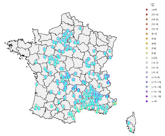
subsequent days and until the end of July at each grid point and then averaged over the
domain. Despite the fact that the average characterizes the mean lowest temperature that can
occur after GDD threshold crossing, the average can mix several dates as the GDD threshold
crossing and the yearly minimum does not necessarily occur on the same date over the whole
domain. In 2021, for instance, the TNnGDD250 was already reached during the 6-8 Apr
episode for most of the area, but not in the easternmost part and in some other parts, because
GDD did not exceed 250°C.day during the April frosts.

In order to focus more on specific phenological periods when young leaves and flowers are
sensitive to frost after bud burst and flowering, we also defined indices over ranges of GDD
values. The number of possibilities are large, in most cases providing similar results. The
analysis is reported here for the range 250-350°C.day. This index is again calculated by grid
points before being averaged spatially, or is taken at stations.

Event attribution methods used in this study are well documented in previous studies. The
general approach follows the classical event attribution probabilistic methodology (Philip et al.,
2020; van Oldenborgh et al., 2021), and has been used in many case studies now for heat
waves (eg. Kew et al., 2019, Vautard et al., 2020), extreme precipitation (eg. Philip et al.,
2018), or more complex events such as wildfire weather (van Oldenborgh et al., 2020). It uses
a stepwise approach analyzing observations with a Generalized Extreme Value (GEV) with
covariate (generally smoothed Global Mean Surface Temperature - GMST or CO2
concentrations as proxies for global warming), using ensembles of models validated on the
event indices and their extreme value statistics by comparison with observations, and then
using the GEV with the covariate fit to build a statistical model of the data under some
assumptions.

For all indices and models, as well as for observations, we used data in the 1951-2021 period
for the GEV fit. For observations, the covariate is the smoothed observed GMST, while for
models the mean surface air temperature of the models is used. In order to study cold
extremes we fit the negative of the indices and transform back. For models we generally used
the mean GSAT of the model itself. The only exception is the High Resolution Model
Intercomparison Project (HighResMIP) SST-forced ensemble, for which the observed GMST
was used.

3. Observations and past trends
The observations used here are the E-OBS v23e dataset of daily minimum temperatures
extended in near real time for 2021. In Figure 3 we show the annual time series of the indices,
together with trend statistics for the 1951-2020 period. We do not take into account 2021 to
avoid selection bias in trend calculation. The Apr-Jul TNn has a slightly upward linear trend of
+0.13°C/Decade, which is however not significant at the 90% (two-sided) level. By contrast,
both TNnGDD250 and TNnGDD250-350 have a significant cooling trend of -0.21 and -
0.25°C/Decade respectively. The warming trend in TNnApr-Jul is partly due to larger values
since 2000, but these higher values are not reflected in the other indices because GDD also
has increased during this period, allowing lower daily minimum temperatures to be counted
earlier in the season. We conclude that, on average, since 1950, extreme yearly minimum
temperatures for GDD>250 have cooled by about 1.5-2.0°C. Very low growing-period frosts
were also found in 1957 and1991, with lower values than in 2021.
For different thresholds we also find cooling trends, however with lower significance. The
significance of the signal remains weak and interannual variability is large. Interestingly, over
the last 50 years (1971-2020) the trends have increased and become more significant (for
instance +0.29°C/Decade, p
E-OBS statistics             TNnApr-Jul          TNnGDD250           TNnGDD250-350           TNnGDD150       TNnGDD350
 0 to 1.2° global warming
 level

 Observed 2021 (°C)           -3.68°C             -2.26°C             -2.24°C                 -3.76°C         1.43°C

 Return Period 2021 (Yr)      160 [25;Inf]        9 [4;28]            16 [6.1;130]            12 [6-110]      2.2 [1.4-3.9]

 Return Period -1.2C (Yr)     10 [5.3;33]         110 [26;inf]        2100 [>65]              39 [>13]        10.0 [4.6;42]

 Probability Ratio            0.06 [0;0.2]        12 [2.0;inf]        130 [>2.4]              3 [>0.6]        4.6 [1.4;23]

 Intensity Change (°C)        +1.4 [0.1;2.6]      -2.0 [-3.2; -       -2.0 [-3.4,-0.45]       -0.80 [-        -1.9 [-3.5,-
                                                  0.7]                                        2.1,0.37]       0.41]

      Table 1: Extreme value statistics and observations for the various indices and
      using the 1951-2020 period and a GEV fit with GMST covariate. Bold font denotes
      statistical significance.

In addition to a domain-average analysis, we calculated trends for 3 specific stations in the
domain (stars in Figure 2). We selected a subset of the Météo-France reference stations,
yielding about 12 stations. To restrict the analysis, we selected 3 stations in grapevine regions
(Beaucouzé: downstream Loire valley; Charnay-les-Mâcon: Burgundy; Charmeil: Saint-
Pourçain grapevine), with several characteristics: for Beaucouzé, light frost and non-
exceptional event (-1.3°C) but high GDD (321°C.day on 5 April); for Charnay-les-Mâcon:
record frost (-4.4°C, with 266°C.day on 5 April), and for Charmeil: the most severe frost among
the 12 regional stations (-6.6°C with 244°C.day on 5 April). Detection results are shown in
Table 2, for these stations. We also restricted the analysis to the three main indices: TNnApr-
Jul, TNnGDD250 and TNnGDD250-350. In almost all cases, the trends are positive for the
fixed season index and negative for the growing season period. However, almost no result is
statistically significant, as variability is dominating the signal (Table 2).

                              Beaucouzé                      Charnay-les-Mâcon                            Charmeil

                     Value              PR                Value              PR                Value           PR
                     Ret. Per.          ∆I
                                                          Ret. Per.          ∆I                Ret. Per.       ∆I

 TNnAprJul           -1.3°C             0.3 [0.02;1.2]    -4.4°C             0.03 [0;0.9]      -6.6°C          0.2 [0.01;7.2]
                     11 yr              1.4 [-0.3;3.0]    >100 yr            1.5 [0.1;2.8]     85 yr           1.2 [-0.7;3.0]

 TNnGDD250           -1.3°C             1.4 [0.2;9.0]     -4.4°C             >1e-4             -5.3°C          3.0 [>0.2]
                     5 yr               -0.4 [-2.2;1.8]   >50 yr             0.2 [-2;2]        18 yr           -1.0 [-3;1]

 TNnGDD250-          -1.3°C             1.1 [0.14;7.2]    -4.4°C             Infinite          -6.6°C          >0.7
                     7 yr               -0.2 [-2.5;2.3]   >90 yr             0.3 [-2.0;2.6]    83 yr           -1.5 [-4;1]
 350

      Table 2: Return periods, probability ratios and changes in intensities obtained from
      the observations at three stations located as in Figure 2b. Red color indicates a
      warming change and blue color a cooling change.
4. Models 4.1 Model ensembles For the attribution of the frost event, we use five model ensembles. The first model ensemble is the Euro-CORDEX (0.11° resolution, EUR-11) multi-model ensemble, composed of 75 combinations (as of May 2021) of Global Climate Models (GCMs) and Regional Climate Models (RCMs) for downscaling (see Vautard et al., 2020 and Coppola et al., 2020 for the description of the ensemble which has increased since these publications). Each simulation consists of a historical period simulation and a RCP8.5 scenario simulation with fixed aerosol concentrations. For the attribution of past evolutions historical and scenario are concatenated until 2020. Some simulations start in 1971, whereas most simulations start from 1951. Given that we need to use data from the previous year for starting GDD accumulation, and that some simulations were terminated in 2099, all yearly indices are calculated from their second simulation year (i.e. for some models in 1972) until 2098. The ensemble was bias-adjusted using the CDFt method (Vrac et al., 2016) using the daily minimum and the daily average temperatures from E-OBS. This method was assessed for use in climate services in Bartok et al. (2019), and showed good performance. We used statistics of the pooled ensemble, using data until 2021 for the GEV fit of the distributions. The second model ensemble used to study the influence of internal variability was the IPSL- CM6A-LR model (see Boucher et al., 2020 for a description of the model). It is composed of 32 extended historical simulations, following the CMIP6 protocol (Eyring et al., 2016) over the historical period (1850-2014) and extended until 2059 using all forcings from the SSP2-4.5 scenario, with the exception of the ozone concentration which has been kept constant at its 2014 climatology (as it was not available at the time of performing the extensions). Then, two other model ensembles were used. The first one is a selection of the CMIP6 historical and SSP3-7.0 simulations. In this case, bias correction was not applied, and we selected the least biased simulations (see Appendix A for details). The second one used is a set of 10 SST-forced HighResMIP simulations (Haarsma et al. 2016). For the historical time period (1950-2014), the SST and sea ice forcings used are based on observed dataset, and for the future time period (2015-2050) the SST and sea ice are derived from CMIP5 RCP8.5 simulations and a scenario as close to RCP8.5 as possible within CMIP6. This ensemble was bias-corrected, as detailed in the Appendix along with the details of each model used here. 4.2 Model evaluation We compared the model GEV fit parameters over the overlapping model periods (1951-2020) in order to check the ability of models to simulate such extremes. Such ability was not confirmed for heat waves (eg. Vautard et al., 2020). In the current case, we found that model ensembles are compatible with the observations accounting for uncertainties (see Table 2) in most cases. We restrict the comparison to 2 indices for simplicity. For TNnGDD250 the fitted model scale parameter is compatible with the observed one except for HiResMip where the variability is too large. The shape parameter is very uncertain in observations, leaving all model fits compatible with them. The same occurs for the TNnApr-Jul, but in this case all models have an overestimated scale parameter (in terms of amplitude). Only Euro-Cordex appears to have a parameter compatible with observations. Given this evaluation, for the final model “weighted average” (see Philip et al., 2020), and to have a homogeneous set of
ensembles only Euro-Cordex will be considered for the statistical evaluation of probability ratio
and intensity change, while for the TNnGDD250 index, all ensembles but the HiResMIP
ensemble will be considered.

 Model ensemble /        Index                    Scale parameter          Shape parameter
 Observation

 Observation             TNnApr-Jul               1.21 [0.93;1.44]         -0.23 [-0.41;-0.03]

 Euro-Cordex                                      1.41 [1.34;1.45]         -0.22 [-0.25;-0.19]

 IPSL-CM6A-LR                                     1.55 [1.50;1.60]         -0.16 [-0.18;-0.13]

 CMIP6                                            1.63 [1.55;1.69]         -0.19 [-0.23;-0.15]

 HiResMIP-SST                                     1.53 [1.46;1.64]         -0.30 [-0.36;-0.27]

 Observation             TNnGDD250                1.43 [1.13;1.65]         -0.19 [-0.54;+0.06]

 Euro-Cordex                                      1.52 [1.45;1.57]         -0.24 [-0.26;-0.23]

 IPSL-CM6A-LR                                     1.19 [1.14;1.22]         -0.18 [-0.22;-0.17]

 CMIP6                                            1.68 [1.59;1.74]         -0.17 [-0.21;-0.14]

 HiResMIP-SST                                     1.96 [1.84;2.08]         -0.11 [-0.18;-0.09]

      Table 2: Model evaluation, using 2 main indices (TNnApr-Jul and TNnGDD250).
      Results for TNnGDD250-350 are qualitatively similar to those for TNnGDD250.

4.3 Simulated mean trends
We analysed the trends in the various indices for growing period frosts for the IPSL ensemble
and the Euro Cordex model ensemble in the form of histograms, in order to examine the
variability across ensemble members. For the other ensembles the number of models is not
large enough hence not shown in the histogram figures. For both ensembles, there is a large
range of minimum temperature trends from April to May, which are almost all positive. The
observed trend in the minimum temperature from April to May is close to the middle of the
distribution for both ensembles. A large range of possibilities is also found for the trends of
minimum temperature based on different GDD thresholds, with a large part of the simulations
showing lower trends than the trends of the minimum temperature from April to May. The
observed strong negative trend in minimum temperature after the GDD>250 threshold over
the period 1971-2020 appears to be a fairly rare case, as it is at the tail end of the distribution
for both ensembles. We conclude from these figures that, despite the general trend towards
cooling of the growing period frosts, the expected trend, for a given singular member, can also
be toward a warming, albeit with a lower chance than for a cooling. This large uncertainty also
has to be taken into account in any adaptation strategy.
Figure 4. Histogram of the daily minimum temperature trend calculated from (a)
the IPSL ensemble, (b) the Euro-Cordex ensemble. The observations are
represented with the vertical lines. The trends are calculated over the 1971-2020
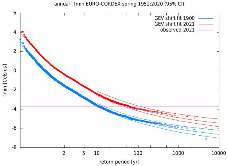
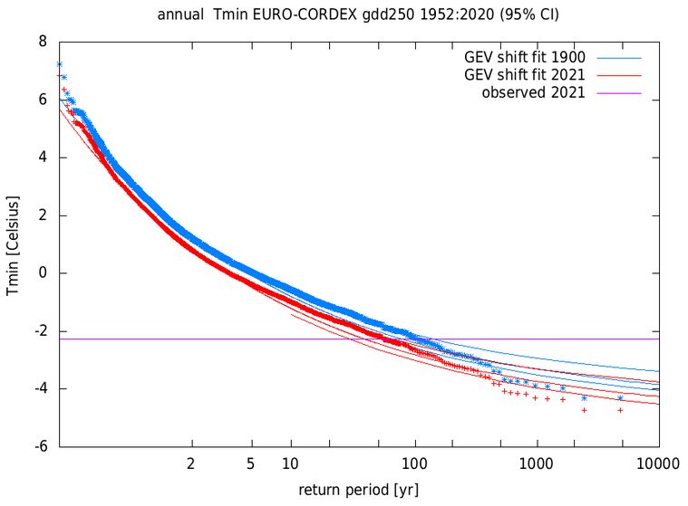
period for (green) GDD>250, (brown) 250Figure 5. Return value vs. return period for EuroCORDEX and the indices
TNnApr-Jul and TNnGDD250.
Model ensemble / Index Probability Intensity
Observation Ratio change (°C)
2021 vs 2021 2021 vs 2021
-1.2°C -1.2°C
Observation TNnApr-Jul RP=160 [>25] 0.06 [8e-5;0.77] +1.4 [0.1;2.6]
Euro-Cordex [75] 2021 vs p.i. 0.20 [0.10;0.30] +1.0 [0.7;1.2]
2C changes relative to 2021 (+0.8°C) 2C vs 2021 0.45 [0.23;0.63] +0.36 [0.2;0.6]
IPSL-CM6A-LR [32] 2021 vs p.i. 0.17 [0.11;0.23] +1.4 [1.2;1.6]
CMIP6 [15] 2021 vs p.i. 0.26 [0.14;0.41] +1.0 [0.7;1.2]
2C changes relative to 2021 (+0.8°C) 2C vs 2021 0.06 [2.0] -2.0 [-3.3, -0.6]
Euro-Cordex 2021 vs p.i. 1.4 [1.0;1.8] -0.30 [-0.56;-0.0]
2C changes relative to 2021 (+0.8°C) 2C vs 1.2C 1.4 [1.1 1.7] -0.34 [-0.50;-0.1]
IPSL-CM6A-LR 2021 vs p.i. 1.5 [1.3;1.9] -0.32 [-0.50;-0.14]
CMIP6 2021 vs p.i. 2.0 [1.6;2.5] -0.78 [-1.0;-0.50]
2C changes relative to 2021 (+0.8°C) 2C vs 1.2C 1.4 [1.1;1.6] -0.33 [-0.5;-0.1]
HiResMip 2021 vs p.i. 1.6 [1.2; 2.5] -0.71 [-1.42;-0.28]
Model average 2021 vs p.i. 1.6 [1.2;2.2] -0.46 [-0.95;+0.04]
2C vs 1.2C 1.4 [1.2;1.6] -0.34 [-0.45;-0.17]Observation TNnGDD150 12 [5;73] 3 [>0.6] -0.80 [-2.2;0.37]
Euro-Cordex 2021 vs p.i. 3.7 [1.2;39] -0.30 [-0.55;-0.03]
IPSL-CM6A-LR 2021 vs p.i. 1.16 [0.91;1.7] -0.09 [-0.30;+0.06]
CMIP6 2021 vs p.i. 0.94 [0.62;1.1] +0.07 [-0.11;0.53]
HiResMip 2021 vs p.i. 1.3 [1.0;1.9] -0.39 [-1.1;0.0]
Observation TNnGDD350 2.2 [1.4;3.9] 4.6 [1.4;23] -1.9 [-3.5;-0.41]
Euro-Cordex 2021 vs p.i. 1.1 [1.0;1.3] -0.30 [-0.59;+0.00]
IPSL-CM6A-LR 2021 vs p.i. 1.9 [1.6;6.7] -0.28 [-0.50;-0.19]
CMIP6 2021 vs p.i. 1.9 [1.6;2.4] -0.99 [-1.4;0.77]
HiResMip 2021 vs p.i. 1.4 [1.0;1.6] -0.71 [-1.2;-0.0]
Observation TNnGDD250- 16 [6.3;120] 130 [>2.4] -2.0 [-3.4;-0.60]
350
Euro-Cordex 2021 vs p.i. 1.6 [1.2;3.0] -0.40 [-0.75;-0.10]
2C changes relative to 2021 (+0.8°C) 2C vs 2021 1.2 [1.0;1.9] -0.14 [-0.49;-0.03]
IPSL-CM6A-LR 1.8 [1.3;2.3] -0.36 [-0.48;-0.15]
CMIP6 2021 vs p.i. 1.3 [0.9;1.6] -0.25 [-0.54;0.06]
2C changes relative to 2021 (+0.8°C) 2C vs 2021 1.5 [1.2;1.9] -0.40 [-0.59;-0.19]
HiResMip 2021 vs p.i. 2.2 [1.1;4.8] -0.74 [-1.3;-0.05]
Model average 1.6 [1.2; 2.0] -0.35 [-0.46; -0.19]
2C changes relative to 2021 (+0.8°C 1.3 [1.2; 1.7] -0.27 [-0.47; -0.15]
Table 3: Extreme value statistics for all model ensembles and observations, with the GEV model fitted from data
over the 1951-2021 period (removing the 2021 value only for the observation) for the past trends estimates, and
over the 2000-2050 period for future trends (when estimating the changes for a 2°C warming above pre-industrial
levels); We assume here that pre-industrial (p.i.) global warming level is -1.2°C cooler than the 2021 one, and
therefore the 2°C is reached 0.8°C above the current level. In each cell, the first line corresponds to the values of
the probability ratio and the intensity change obtained by using the same return period threshold as in the
observation. This is done only in case of large discrepancy with observation return period. Numbers in blue indicate
a decrease of TN, and in red an increase of TN. The last row indicates changes for a 2C warming level. Boldface
numbers indicate statistical significance against a “no change” assumption.
Despite a qualitative agreement between models and observations on trends, models
generally simulate weaker trends for the GDD-conditioned indices than observed, a fact thatremains as of today unexplained, just as the underestimation in extreme temperatures in
summer heat waves (see eg. Vautard et al., 2020; van Oldenborgh et al., in preparation).
4.5 Future trends
Minimum temperatures in spring or in the growing season are projected to have similar trends
as in the past decades in the ensembles and scenarios considered here. Figure 6 shows
evolutions of the ensemble-median and 10th and 90th percentiles for the ensembles having
future trends in different scenarios (Euro-Cordex RCP8.5; CMIP6n SSP3-7.0). In both cases,
the median of yearly minimum temperatures over the region continue to increase with mean
values around 2°C while they are below frost level in 2021. By the end of the century, frost
such as in 2021 will become a very rare occurrence in April or after in these scenarios.
However, frost can be expected earlier in the year, while at the same time the e growing
season starts earlier. This can be seen in the development of the TNnGDD250 index
throughout the 21st century which shows a weak decreasing trend. It is noteworthy that in the
second half of the century, the 90th percentile often nears or exceeds the 2021 value. More
frequent events like the 2021 are therefore expected.
Figure 6. Time evolution of the median (thick line), and the 10th and 90th
percentiles (dashed lines) of the ensembles Euro-Cordex (75 members) and
CMIP6 (15 members) for the indices TNnApr-Jul (Red) and TNnGDD250 (blue).
The thick dashed lines represent the values reached in 2021 for each of the
indices.
In order to quantify these future trends using the global-warming level conditioned GEV fit, we
restrict the analysis to the 2°C warming level above the preindustrial conditions, which is
assumed to be 0.8°C above current level. This restriction is made to be on the safe side with
potential nonlinearity of response of the extreme indices to global warming. Such nonlinearity
is suggested in Figure 6 (left) for the Euro-Cordex model, with a steeper decrease of
TNnGDD250 after the year 2000. The analysis is also restricted to Euro-Cordex and CMIP6
as these ensemble are homogeneous across time (HiResMIP here is forced by observed
SSTs until 2014 and GCM SSTs beyond) and have enough future data (IPSL-CM6A-LR only
has data until 2030). In this future case the GEV fit is carried out over the 2000-2050 period,
and probability ratios and intensity changes are given for events with a similar return period
as the 2021 event.Results are shown along with attribution results in Table 3 . Extreme frosts beyond April 1st will continue to become less extreme. Euro-Cordex simulations project that the 2021 event, considered as a fixed-season minimum, will become about twice less frequent [factor between 1.5 and 3] in a 2°C warmer climate, while the CMIP6 selection projects a reduction by a larger factor (between 3 and 50). In contrast, the growing-period extreme frost intensity is increasing, and the 2021 event with a GDD>250 is projected to have an increasing frequency by about 30% [10% - 60%] for a 2°C warmer climate than preindustrial, in Euro-Cordex, and 40% [10%- 60%] for CMIP6 selections. The early growing season minimum temperatures frequency follow a similar evolution as the growing period extreme frost (see Table 3 and Figure 8).
5. Synthesis, summary and discussion
In Figure 7 we summarise the results of all the individual assessments described above for
probability ratio and intensity change in the historical period. Given the large differences
between models and observations for the growing-period indices TNnGDD250 and
TNnGDD250-350, we do not combine the observational and model results to form a
"synthesis" but instead we present the model weighted average for comparison with the
observations. In the case of the first index, TNnApr-Jul, we also do not form a synthesis
because only one model (ensemble), Euro-Cordex, passes the validation criteria. However,
the two additional models (IPSL-CM6A-LR and CMIP6) that validate well for TNnGDD250 and
TNnGDD250-350, give similar results to Euro-Cordex. Incorporating them in the weighted
average allows a term for model spread to be included which, whilst having little impact on the
best estimate, should improve the uncertainty assessment.

While uncertainties are comparably large for the quantitative assessment of probability ratios
there is a significant decrease in the likelihood of cold waves as defined above for TNnApr-
Jul. The event that has occurred in 2021, taken as a fixed-season extreme, has become
extremely rare, with a return period of at least 25 years, and with a best estimate of 160 years.
The intensity of a cold wave as observed in April is also decreasing, by a well-constrained
best estimate of 1.2°C. For the GDD-based indices models and observations quantitatively
disagree with respect to probability ratio and intensity, the qualitative results are however clear
and show an increase in the likelihood of damaging frost as well as an increase in the intensity
across all indices. A result that is corroborated by the fact that these trends continue under
future warming (see below). This allows for a clear qualitative attribution of these trends to
anthropogenic climate change with the model results serving as lower bounds.

In Figure 8 we summarise the projected changes in probability and intensity between the
present and +2°C climate, showing an unweighted average for the two model ensembles
Euro-Cordex and CMIP6. Note that the CMIP6 selected ensemble did not pass the validation
over the historical period for the first index, TNnApr-Jul, but it is included here as (i) it is
included for the other two indices and we do not know how well it validates for the future, (ii)
no synthesis is formed so the unweighted average shown is only of qualitative use. Probability
ratios are less than unity for TNnApr-Jul, indicating that the current trend for decreasing
frequency of cold snaps is likely to continue in the future. Projections indicate a decrease by
a factor of about 5 in the type of event witnessed in 2021. Likewise, the projections for change
in intensity indicate that Apr-Jul cold snaps will continue to warm, by a best-estimated increase
of about 0.6°C. Growing-period minimum temperatures continue to decrease with a best
estimate of about 0.3°C and an increase in frequency of about 40% with some variations
among indices.
Figure 7. Changes between the past and present: summary of observational
(blue) and model (red) results for probability ratio (left) and change in intensity [°C]
(right) in the three indices TNnApr-Jul (top), TNnGDD250 (middle) and
TNnGDD250-350 (bottom). Extent of the bars gives 95% confidence intervals
accounting for variability within the data sets and model spread (white) where
appropriate, with the black marker indicating the best estimate. A weighted
average of model results is shown in bright red. Note that, for the index TNnApr-
Jul, only Euro-Cordex passed the validation step but other models are included in
the weighted average for reasons described in the text.

Figure 8. Projected changes between the present and +2degC climate: summary
of results for probability ratio (left) and change in intensity [°C] (right) in the three
indices TNnApr-Jul (top), TNnGDD250 (middle) and TNnGDD250-350 (bottom).
Extent of the bars gives 95% confidence intervals accounting for variability within
the data sets, with the black marker indicating the best estimate. An unweighted
average of the results is shown in bright red.
While the growing season is starting earlier, necessary plant dormancy characteristics also
change and the lack of chilling winter days may delay the bud burst in many species (Chuine
et al., 2016). This effect is not taken into account here and could alter our results concerning
changes in bud burst dates. Such dates are also dependent on species. We have tested the
dependence on thresholds of a simple GDD index, which provide similar results than the
central thresholds discussed in the synthesis. Dormancy effects, as well as other specific plant
effects can only be studied through impact models, which was not the goal in this study.

The applicability of our results at local scale is limited in quantitative terms. The local station
analysis, and the trends histograms show that given locations are more likely to exhibit cooling
of extreme growing-period temperatures than warming, but a warming cannot be excluded at
these scales and at present day warming levels.

The discrepancy between trends in models and in observations in the historical periods
currently remains unexplained. It shows that either large variability inhibits an accurate
estimation of trends of cold extremes or that other factors come into play which may not be
well simulated such as trends in radiation or cloudiness as a response to either warming or
aerosols. These factors should be investigated in future studies.

Above all, the finding that trends identified up until now continue under future warming
indicates that anthropogenic climate change is an important driver of the observed trends and
suggests that the models indeed underestimate the effect of change due to forcing factors and
that the discrepancy between observed and simulated trends is not entirely explainable by
unmodelled factors other than human-induced climate change.

In conclusion, we identify two key attributable effects, the decrease in likelihood and intensity
of minimum temperatures and the increase of likelihood and intensity of minimum
temperatures when conditioned on growing degree indices. These findings are consistent
across the different lines of evidence pursued despite the quantitative differences. The GDD-
indices are however a crude representation of the vulnerability of different species to frost.
Thus, our findings highlight that growing season frost damage is a potentially extremely costly
impact of climate change already damaging the agricultural industry but to inform adaptation
strategies for specific species impact-based modelling will need to complement our
assessment.
Annex I. Model ensembles description
This annex provides more details about the model ensembles used in this study.

1. EURO-CORDEX
The Euro-Cordex ensemble is made of 75 simulations of 12 Regional climate models
downscaling 8 Global Climate Models. The description of the ensemble is detailed in Vautard
et al. (2021) and Coppola et al. (2020), but since this article publication the ensemble size
passed from 55 models to 75 models. The reader is referred to this publication for a description
and an assessment of this ensemble in the historical period. Daily mean and minimum
temperatures were corrected at grid point level using the E-OBS observation dataset from
1981 to 2020. Bias correction follows the method described in Vrac et al. (2016) refined in
Bartok et a. (2019) and applied on daily data instead of hourly data.

2. CMIP6 selected ensemble
The CMIP6 multi-model ensemble is a set of global climate models, developed by several
institutes around the world (Eyring et al., 2016). Here a subset of CMIP6 models are used,
with historical and SSP2-4.5 experiments (Meehl et al. 2014; O’Neill et al. 2014, Vuuren et al.
2014, and O’Neill et al. 2016) together spanning the period between 1850 and 2099 for tas
and tasmin variables.

In this case simulations were not bias-corrected but, instead, a selection of the least biased
models was made together with a restriction to 3 members maximum for the ensemble. This
is due to the fact that there was a large heterogeneity in the number of members for each
model in CMIP6, and to avoid giving too much weight to a particular model.

The selection criterion is the bias in both TNnApr-Jul and TNnGDD250 indices over the 1971-
2020 period. Typically, models biased by less than 2°C were kept. This led to 15-member
multimodel ensemble with a selection of the following models: CanESM5 (3 members),
CNRM-CM6-1 (1 member), CNRM-ESM2-1 (1 member), ACCESS-CM2 (3 members), EC-
Earth3-AerChem (2 members), EC-Earth3-Veg (2 members).

3. IPSL-CM6 single model ensemble
The IPSL-CM6A-LR model ensemble is a 32-member ensemble of the coupled climate model
with the same name. The model is described in Boucher et al. (2020). Simulations start in the
pre-industrial with slightly different initial conditions and are saved in this study for the whole
historical period and beyond, until 2029. The ensemble has been used for attribution studies,
for instance in the 2019 heatwave attribution described in Vautard et al. (2020).

4. HighresMIP SST-forced ensemble
The six HighResMIP models are: 1) CNRM-CM6-1-HR, 1 simulation is used, run by the CNRM
(Centre National de Recherches Meteorologiques), CERFACS (Centre Europeen de
Recherche et de Formation Avancee en Calcul Scientifique) (CNRM-CERFACS); 2) CNRM-
CM6-1, run by CNRM-CERFACS; 3) EC-Earth3P-HR, 3 simulations are used, run by EC-
Earth-Consortium; 4) EC-Earth3P (EC-Earth 3.2), 3 simulations are used, run by EC-Earth-
Consortium; 5) HadGEM3-GC31-HM(HadGEM3-GC3.1-N512ORCA025), 1 simulation is
used, run by the Met Office Hadley Centre; and 6) HadGEM3-GC31-HM (HadGEM3-GC3.1-
N216ORCA025), 1 simulation is used, run by the Met Office Hadley Centre.

Bias correction was performed on the HighResMIP simulations, using E-OBS (1981-2010) as
reference. Daily mean temperature, minimum temperature, and GDD were bias-corrected
respectively before the other indices were calculated, and each month was correctly
separately. All the calculations were done on a grid-point base, then averaged spatially over
the studied region.

Table A1. Spatial grids of the HighresMIP models in high-, medium,-, and low-resolution
groups used in this study.

 Model             High               Medium            Low                DOI

 CNRM-CM6-1-                          720*360                              https://doi.org/1
 HR                                                                        0.22033/ESGF/
                                                                           CMIP6.1387
 CNRM-CM6-1                                             256*128            https://doi.org/1
                                                                           0.22033/ESGF/
                                                                           CMIP6.1375
 EC-Earth3P-HR     1024*512                                                https://doi.org/1
                                                                           0.22033/ESGF/
                                                                           CMIP6.2323
 EC-Earth3P                           512*256                              https://doi.org/1
                                                                           0.22033/ESGF/
                                                                           CMIP6.2322
 HadGEM3-          1024*768                                                https://doi.org/1
 GC31-HM                                                                   0.22033/ESGF/
                                                                           CMIP6.446
 HadGEM3-                             432*324                              https://doi.org/1
 GC31-MM                                                                   0.22033/ESGF/
                                                                           CMIP6.1902
Acknowledgements We are grateful to Iñaki Garcia de Cortazar Atauri for fruitful discussions and further references for this article. We are also grateful to James Ciarlo (ICTP) who made available in advance to publication on ESGF one of the regional climate simulations for the Euro-Cordex ensemble. The analysis benefitted from the collection of the Euro-Cordex simulation made within the Copernicus Climate Change Service. Related literature Barnes, E.A. and Screen, J.A. (2015), The impact of Arctic warming on the midlatitude jet- stream: Can it? Has it? Will it?. WIREs Clim Change, 6: 277-286. https://doi.org/10.1002/wcc.337 Bartok, B., Tobin, I., Vautard, R., Vrac, M., Jin, X., Levavasseur, G., ... & Saint-Drenan, Y. M. (2019). A climate projection dataset tailored for the European energy sector. Climate services, 16, 100138. Besson F., Dubuisson B., Etchevers P., Gibelin A.-L., Lassegues P., Schneider M., Vincendon B., (2019). Climate monitoring and heat and cold waves detection over France using a new spatialization of daily temperature extremes from 1947 to present. Adv. Sci. Res. 16, 149-156. doi: 10.5194/asr-16-149-2019 Boucher, O., Servonnat, J., Albright, A. L., Aumont, O., Balkanski, Y., Bastrikov, V., ... & Vuichard, N. (2020). Presentation and evaluation of the IPSL-CM6A-LR climate model. Journal of Advances in Modeling Earth Systems, 12(7), e2019MS002010. Chuine, I., Bonhomme, M., Legave, J. M., García de Cortázar-Atauri, I., Charrier, G., Lacointe, A., & Améglio, T. (2016). Can phenological models predict tree phenology accurately in the future? The unrevealed hurdle of endodormancy break. Global Change Biology, 22(10), 3444- 3460. Coppola, E., Nogherotto, R., Ciarlo', J. M., Giorgi, F., van Meijgaard, E., Kadygrov, N., ... & Wulfmeyer, V. (2021). Assessment of the European climate projections as simulated by the large EURO-CORDEX regional and global climate model ensemble. Journal of Geophysical Research: Atmospheres, 126(4), e2019JD032356. EC-Earth Consortium (EC-Earth) (2018). EC-Earth-Consortium EC-Earth3P-HR model output prepared for CMIP6 HighResMIP. Version 20201214[1].Earth System Grid Federation. https://doi.org/10.22033/ESGF/CMIP6.2323. EC-Earth Consortium (EC-Earth) (2019). EC-Earth-Consortium EC-Earth3P model output prepared for CMIP6 HighResMIP. Version 20201214[1].Earth System Grid Federation. https://doi.org/10.22033/ESGF/CMIP6.2322. Eyring, V., S. Bony, G. A. Meehl, C. A. Senior, B. Stevens, R. J. Stouffer, and K. E. Taylor (2016). “Overview of the Coupled Model Intercomparison Project Phase 6 (CMIP6) experimental design and organization”. In: Geosci. Model Dev. 9.5, pp. 1937–1958. doi: 10.5194/gmd-9-1937-2016. Garcia de Cortazar-Atauri et al., 2009 - Int J Biometeorol (2009) 53:317–326. doi: 10.1007/s00484-009-0217-4
Haarsma, R. J., Roberts, M. J., Vidale, P. L., Senior, C. A., Bellucci, A., Bao, Q., ... & Storch,
J. S. V. (2016). High resolution model intercomparison project (HighResMIP v1. 0) for CMIP6.
Geoscientific Model Development, 9(11), 4185-4208.

Kew, S. f., Philip, S. Y., Jan van Oldenborgh, G., van der Schrier, G., Otto, F. E. L., & Vautard,
R. (2019). The Exceptional Summer Heat Wave in Southern Europe 2017, Bulletin of the
American Meteorological Society, 100(1), S49-S53. doi:10.1175/BAMS-D-18-0109.1

Liu, Q., Piao, S., Janssens, I. A., Fu, Y., Peng, S., Lian, X. U., ... & Wang, T. (2018). Extension
of the growing season increases vegetation exposure to frost. Nature Communications, 9(1),
1-8.

Meehl, G. A., R. Moss, K. E. Taylor, V. Eyring, R. J. Stouffer, S. Bony, and B. Stevens (2014).
“Climate Model Intercomparisons: Preparing for the Next Phase”. In: Eos Trans. AGU 95.9,
pp. 77–78. doi: 10.1002/2014EO090001.

Michelangeli, P. A., Vautard, R., & Legras, B. (1995). Weather regimes: Recurrence and quasi
stationarity. Journal of Atmospheric Sciences, 52(8), 1237-1256.

O’Neill, B. C., E. Kriegler, K. Riahi, K. L. Ebi, S. Hallegatte, T. R. Carter, R. Mathur, and D. P.
van Vuuren (2014). “A new scenario framework for climate change research: the concept of
shared socioeconomic pathways”. In: Clim. Change 122.3, pp. 387–400. doi: 10.1007/s10584-
013-0905- 2.

O’Neill, B. C., C. Tebaldi, D. P. van Vuuren, V. Eyring, P. Friedlingstein, G. Hurtt, R. Knutti, E.
Kriegler, J.-F. Lamarque, J. Lowe, G. A. Meehl, R. Moss, K. Riahi, and B. M. Sanderson
(2016). “The Scenario Model Intercomparison Project (ScenarioMIP) for CMIP6”. In: Geosci.
Model Dev. 9.9, pp. 3461–3482. doi: 10.5194/gmd-9-3461-2016.

Philip, S., Kew, S., van Oldenborgh, G. J., Otto, F., Vautard, R., van der Wiel, K., King, A.,
Lott, F., Arrighi, J., Singh, R., and van Aalst, M.: A protocol for probabilistic extreme event
attribution analyses,        Adv. Stat.    Clim. Meteorol. Oceanogr., 6, 177–203,
https://doi.org/10.5194/ascmo-6-177-2020, 2020.

Roberts, Malcolm (2017). MOHC HadGEM3-GC31-HM model output prepared for CMIP6
HighResMIP.         Version    20210407[1].Earth System   Grid     Federation.
https://doi.org/10.22033/ESGF/CMIP6.446.

Roberts, Malcolm (2017). MOHC HadGEM3-GC31-MM model output prepared for CMIP6
HighResMIP.         Version    20210407[1].Earth System   Grid     Federation.
https://doi.org/10.22033/ESGF/CMIP6.1902.

Screen, J. A., and Simmonds, I. (2013), Exploring links between Arctic amplification and mid-
latitude weather, Geophys. Res. Lett., 40, 959–964, doi:10.1002/grl.50174.

Sgubin, G., Didier Swingedouw, Gildas Dayon, Iñaki García de Cortázar-Atauri, Nathalie Ollat,
Christian Pagé, Cornelis van Leeuwen, The risk of tardive frost damage in French vineyards
in a changing climate, Agricultural and Forest Meteorology, Volumes 250–251, 2018, Pages
226-242, ISSN 0168-1923, https://doi.org/10.1016/j.agrformet.2017.12.253
Van Oldenborgh, G.J., van der Wiel, K., Kew, S. et al. Pathways and pitfalls in extreme event
attribution. Climatic Change, 166, 13, https://doi.org/10.1007/s10584-021-03071-7, 2021.

van Vuuren, D. P. van, E. Kriegler, B. C. O’Neill, K. L. Ebi, K. Riahi, T. R. Carter, J. Edmonds,
S. Hallegatte, T. Kram, R. Mathur, and H. Winkler (2014). “A new scenario framework for
Climate Change Research: scenario matrix architecture”. In: Clim. Change 122.3, pp. 373–
386. doi: 10. 1007/s10584-013-0906-1.

Vautard, R. (1990). Multiple weather regimes over the North Atlantic: Analysis of precursors
and successors. Monthly weather review, 118(10), 2056-2081.

Vautard, R., van Aalst, M., Boucher, O., Drouin, A., Haustein, K., Kreienkamp, F., ... & Wehner,
M. (2020). Human contribution to the record-breaking June and July 2019 heatwaves in
Western Europe. Environmental Research Letters, 15(9), 094077.

Vautard, R., Kadygrov, N., Iles, C., Boberg, F., Buonomo, E., Bülow, K., ... & Wulfmeyer, V.
(2020). Evaluation of the large EURO-CORDEX regional climate model ensemble. Journal of
Geophysical           Research:         Atmospheres,          e2019JD032344.            doi:
https://doi.org/10.1029/2019JD032344

Voldoire, Aurore (2019). CNRM-CERFACS CNRM-CM6-1-HR model output prepared for
CMIP6       HighResMIP.    Version   20210407[1].Earth System Grid Federation.
https://doi.org/10.22033/ESGF/CMIP6.1387.

Voldoire, Aurore (2018). CNRM-CERFACS CNRM-CM6-1 model output prepared for CMIP6
CMIP.          Version      20210407[1].Earth System       Grid       Federation.
https://doi.org/10.22033/ESGF/CMIP6.1375.

Vrac, M., Noël, T., & Vautard, R. (2016). Bias correction of precipitation through Singularity
Stochastic Removal: Because occurrences matter. Journal of Geophysical Research:
Atmospheres, 121(10), 5237-5258.
You can also read