Teleconnections and Extreme Ocean States in the Northeast Atlantic Ocean
←
→
Page content transcription
If your browser does not render page correctly, please read the page content below
18th EMS Annual Meeting: European Conference for Applied Meteorology and Climatology 2018
Adv. Sci. Res., 16, 11–29, 2019
https://doi.org/10.5194/asr-16-11-2019
© Author(s) 2019. This work is distributed under
the Creative Commons Attribution 4.0 License.

              Teleconnections and Extreme Ocean States in the
                         Northeast Atlantic Ocean
       Emily Gleeson1 , Colm Clancy1 , Laura Zubiate1 , Jelena Janjić2 , Sarah Gallagher1,2 , and Frédéric Dias2,3
                                 1 Met
                                  Éireann, 65/67 Glasnevin Hill, Dublin 9, D09Y921, Ireland
                      2 School
                             of Mathematics and Statistics, University College Dublin, Dublin, Ireland
                        3 CMLA, ENS Cachan, CNRS, Université Paris-Saclay, 94235 Cachan, France

                                   Correspondence: Emily Gleeson (emily.gleeson@met.ie)

                        Received: 10 December 2018 – Accepted: 1 March 2019 – Published: 22 March 2019

       Abstract. The Northeast Atlantic possesses an energetic and variable wind and wave climate which has a large
       potential for renewable energy extraction; for example along the western seaboards off Ireland. The role of
       surface winds in the generation of ocean waves means that global atmospheric circulation patterns and wave
       climate characteristics are inherently connected. In quantifying how the wave and wind climate of this region
       may change towards the end of the century due to climate change, it is useful to investigate the influence of large
       scale atmospheric oscillations using indices such as the North Atlantic Oscillation (NAO), the East Atlantic
       pattern (EA) and the Scandinavian pattern (SCAND). In this study a statistical analysis of these teleconnections
       was carried out using an ensemble of EC-Earth global climate simulations run under the RCP4.5 and RCP8.5
       forcing scenarios, where EC-Earth is a European-developed atmosphere ocean sea-ice coupled climate model.
       In addition, EC-Earth model fields were used to drive the WAVEWATCH III wave model over the North Atlantic
       basin to create the highest resolution wave projection dataset currently available for Ireland. Using this dataset
       we analysed the correlations between teleconnections and significant wave heights (Hs ) with a particular focus
       on extreme ocean states using a range of statistical methods. The strongest, statistically significant correlations
       exist between the 95th percentile of significant wave height and the NAO. Correlations between extreme Hs and
       the EA and SCAND are weaker and not statistically significant over parts of the North Atlantic. When the NAO
       is in its positive phase (NAO+) and the EA and SCAND are in a negative phase (EA−, SCAND−) the strongest
       effects are seen on 20-year return levels of extreme ocean waves. Under RCP8.5 there are large areas around
       Ireland where the 20-year return level of Hs increases by the end of the century, despite an overall decreasing
       trend in mean wind speeds and hence mean Hs .

1   Introduction                                                   and Livezey, 1987; Wang and Swail, 2001, 2002; Charles
                                                                   et al., 2012; Bertin et al., 2013; Dodet et al., 2010; Atan
The Northeast Atlantic has an energetic, variable wind and         et al., 2016; Santo et al., 2016a). The Scandinavian telecon-
wave climate with a significant potential for renewable en-        nection pattern (SCAND) and East Atlantic Western Rus-
ergy applications (Gallagher et al., 2013; Gallagher et al.,       sian (EA/WR) pattern are other modes of Northern Hemi-
2016b; Atan et al., 2016). Global atmospheric circulation          sphere atmospheric variability, and along with the EA have
patterns and wave climate characteristics are inherently con-      a weaker, but nevertheless significant, influence on the North
nected through the role of surface winds in the genera-            Atlantic than the NAO (Santo et al., 2016b). In particular, the
tion of ocean waves. Several previous studies have shown           EA and SCAND have been found to have an impact on the re-
strong correlations between the wave climate of the North          lationship between the NAO and European precipitation pat-
Atlantic Ocean and atmospheric teleconnection patterns such        terns (Comas-Bru and McDermott, 2014), and wind energy
as the North Atlantic Oscillation (NAO) and the East At-
lantic teleconnection pattern (EA) (for example, Barnston

Published by Copernicus Publications.
12                                                               E. Gleeson et al.: Extreme Ocean States Northeast Atlantic

resources (Zubiate et al., 2017) in winter, by modulating the     ond and third EOFs often interchangeably correspond to ei-
location and relative intensity of the NAO centres of action.     ther the EA or SCAND and are identifiable using a plot of
   A strong link between low-frequency modes of atmo-             the particular 2-D EOF.
spheric variability and mean significant wave height (Hs ),           The study presented in this paper extends the analysis of
wave period and peak direction of the waves in Irish coastal      Gleeson et al. (2017). Here we include the three most dom-
waters was identified by Gallagher et al. (2014). The influ-      inant modes of northern hemisphere atmospheric variabil-
ence of the NAO on extreme sea states in the Northeast At-        ity – the NAO, the EA and the SCAND and employ the
lantic Ocean was investigated by Gleeson et al. (2017) ex-        EOF analysis method in their calculation. The analysis was
plaining how this may change in the future using an ensem-        carried out for the following North Atlantic area 20–90◦ N
ble of WAVEWATCH III (Tolman, 2014) simulations driven            80◦ W–40◦ E using a 3-member ensemble of historical and
by output from the Coupled Model Intercomparison Project          RCP4.5/8.5 projection EC-Earth data for the months of De-
5 (CMIP5) (Taylor et al., 2012) climate simulations carried       cember to March. It is important to note that our ensemble
out using the EC-Earth (Hazeleger et al., 2010, 2012) global      size is small. This was due to the computational demands re-
climate model.                                                    quired to run the very high resolution wave simulations.
   The Gleeson et al. (2017) study focused on the NAO,                The EA was first described by Wallace and Gutzler (1981).
which is the leading mode of atmospheric variability in the       It is defined by a centre of positive 500 hPa height anomalies
North Atlantic region and is manifested as a meridional           around the subtropical North Atlantic. It is known to play
dipole in mean sea-level pressure (MSLP), with centres of         a role, with the NAO, in determining the latitude and ex-
action over Iceland and the Azores (Hurrell, 1996; Great-         tent of the jet stream, and therefore, the main Atlantic storm
batch, 2000; van Loon and Rogers, 1978). Variations in            track (Woollings and Blackburn, 2012). In its negative phase
the amplitude and phase of the NAO are linked to changes          (negative MSLP anomalies in the mid Atlantic) the EA is
in the intensity and frequency of storms and blocking pat-        known to contribute to northwest swells in the Bay of Bis-
terns (Scherrer et al., 2006). A positive NAO phase is as-        cay (Izaguirre et al., 2010).
sociated with a stronger pressure gradient over the North             The SCAND was defined by Barnston and Livezey (1987)
Atlantic, stronger westerly winds and larger waves. On the        as the Eurasia-1 pattern. It is characterised by high pressure
other hand, a negative NAO phase is associated with a weaker      anomalies over the Scandinavian Peninsula and a more dif-
pressure gradient, slacker winds and smaller waves. Glee-         fuse centre of opposite sign over Greenland. It corresponds to
son et al. (2017) showed that the 95th percentile of Hs is        the Scandinavian blocking regime identified in anticyclonic
strongly positively correlated to the NAO, where the station-     set-ups, and is associated with colder than average winter
based interpretation of NAO was employed. Projections of          temperatures and higher occurrences of easterly winds over
Hs extremes were found to be location dependent; under the        Western Europe (Vautard, 1990). This pattern is known to be
influence of positive NAO, the return levels of Hs may in-        negatively correlated with wind speeds and significant wave
crease in the future despite the overall decreasing trend in      heights during at least the extended winter months (Trigo
the projections of Hs .                                           et al., 2008).
   The most commonly used calculation of the NAO index                The paper is organised as follows: Sect. 2 provides details
uses the station-based definition which involves the differ-      about the EC-Earth and WAVEWATCH III models used in
ence between MSLP anomalies in the Icelandic Low and              this study. The atmospheric teleconnections are described in
Azores High action regions (Hurrell, 1996; Pokorná and            more detail in Sect. 3. In Sect. 4 the results of the various
Huth, 2015). This definition was used in Gleeson et al. (2017)    statistical tests are presented and discussed. Conclusions on
and applied to the EC-Earth gridded MSLP fields (using the        the findings of this study are presented in Sect. 5.
nearest grid point to the location of interest). Disadvantages
of this method are that it is fixed in space and shows low        2     Models
signal-to-noise ratios.
   An alternative method for deriving the NAO index in-           The work presented in this paper used data from
volves calculating the principal component (PC) time series       CMIP5 (Taylor et al., 2012) simulations carried out using
of the leading empirical orthogonal function (EOF) of grid-       version 2.3 of the EC-Earth (Hazeleger et al., 2010, 2012)
ded MSLP or 500 hPa geopotential height fields spanning           global climate model to drive the WAVEWATCH III wave
an area bounded by 20–90◦ N and 80◦ W–40◦ E. Note that            model (Tolman, 2014). Details on each of these models are
this method is particularly sensitive to the spatial domain       provided in Gleeson et al. (2017) but a summary is repeated
and time period used. The PC of the second leading EOF            here for completeness.
is usually the East Atlantic (EA) pattern which has a cen-
tre of action in the Atlantic Ocean west of Ireland; the third
                                                                  2.1    EC-Earth climate simulations
leading mode is usually the Scandinavian (SCAND) pattern.
However, these modes often account for approximately the          The EC-Earth global climate model used for the CMIP5
same percentage of atmospheric variability and thus the sec-      climate simulations consists of an atmosphere-land surface

Adv. Sci. Res., 16, 11–29, 2019                                                              www.adv-sci-res.net/16/11/2019/
E. Gleeson et al.: Extreme Ocean States Northeast Atlantic                                                                        13

module coupled to an ocean-sea ice module (Hazeleger et al.,     Table 1. Table explaining the logic behind the experiment names
2010, 2012). The atmospheric component of the model was          used in this paper. The last number in the name refers to the ensem-
based on the European Centre for Medium-Range Weather            ble member. The third letter identifies whether the data refer to the
Forecasts (ECMWF) Integrated Forecasting System (hori-           historical period (i) or were generated under RCP4.5 (4) or RCP8.5
zontal resolution of 1.125◦ or approximately 125 km and          (8). Under RCP4.5 greenhouse gas emissions are expected to peak
                                                                 around the year 2040 and decline after that. Under RCP8.5 green-
62 vertical layers up to 5 hPa). The Nucleus for European
                                                                 house gas emissions are expected to increase throughout the 21st
Modelling of the Ocean (NEMO) version 2 was used for the         century.
oceanic component (Madec, 2008) with an average horizon-
tal resolution of 1◦ (approximately 110 km) and 42 vertical                 Ensemble     Historical    RCP4.5     RCP8.5
levels. The sea-ice component was the Louvain-la-Neuve Sea                  member
Ice Model (LIM) version 2 (Fichefet and Maqueda, 1997).
The Ocean Atmosphere Sea Ice Soil coupler (OASIS) ver-                      1            mei1          me41       me81
sion 3 (Valcke, 2006) was used to couple the atmosphere-                    2            mei2          me42       me82
                                                                            3            mei3          me43       me83
land surface module with the ocean-sea ice module.
   The EC-Earth CMIP5 climate simulations span the pe-
riod 1850 to 2100. The years 1850 to 2009 are classified as
the historical period and included observed greenhouse gases     2070–2099 (for both RCP4.5 and RCP8.5) and the histori-
and aerosol concentrations such as black carbon and volcanic     cal/industrial period 1980–2009.
eruptions. The future period span from 2006 to 2100 under           The following nomenclature is used throughout this pa-
both RCP4.5 and RCP8.5 CMIP5 climate forcing scenarios.          per when referring to the ensemble members and the his-
3 of the 14 EC-Earth CMIP5 ensemble members were gen-            torical and future periods. Each ensemble member consists
erated by Met Éireann and available for use in generating the    of an historical simulation and 2 future simulations (RCP4.5
high resolution wave dataset for Ireland. The EC-Earth en-       and RCP8.5) and are denoted meiX, me4X and me8X where
semble does not have a large spread in terms of annual mean      X = 1, 2, 3 denotes the ensemble member, “i” refers to the
wind speeds and the three Met Éireann ensemble members           historical or industrial period, 4 and 8 refer to RCP4.5 and
encapsulate the range of interannual variability.                RCP8.5 respectively and “me” denotes the fact that it is a
                                                                 Met Éireann ensemble member. This is also summarised in
2.2   WAVEWATCH III simulations                                  Table 1.

WAVEWATCH III is a third-generation “phase-averaged”
model based on a stochastic representation of the sea sur-       3   Atmospheric teleconnections
face solving the wave-action balance equation (Komen et al.,
1994). The evolution of the wave energy spectrum in the          We considered the first three modes of MSLP variability for
presence of currents and bathymetry is described through         a Northern Hemisphere region spanning 20–90◦ and 80◦ W–
the conservation of action density (advection and refraction),   40◦ E using the 3-member EC-Earth ensemble consisting of
which is balanced by source terms (Janssen, 2008). The dissi-    3 historical periods (mei1, mei2, mei3), 3 future periods un-
pation and source term parameterisations formulated in Ard-      der RCP4.5 (me41, me42, me43) and 3 future periods un-
huin et al. (2010) were used in this study.                      der RCP8.5 (me81, me82, me83). The months of December
   EC-Earth 10 m wind speeds and sea-ice fields (Gleeson         through to March were used in the calculations and analysis.
et al., 2013) were used to drive the ensemble of nested re-      For comparison, MSLP variability was also computed using
gional wave projections over the North Atlantic (see Fig. 1).    the ERA-Interim reanalysis dataset.
The outermost grid was a regular grid of 0.75◦ × 0.75◦ res-         We used Empirical Orthogonal Function (EOF) analysis
olution over the North Atlantic; the second grid covered         to examine the variability in the EC-Earth MSLP fields for
part of the Northeast Atlantic on a 0.25◦ × 0.25◦ regular        the periods mentioned above. This multivariate statistical
grid and the innermost grid centred around Ireland was           technique is used in order to reduce the dimensionality of
unstructured (Roland, 2008) with a resolution of approxi-        a dataset containing numerous related variables and at the
mately 15 km at the grid boundaries increasing to 1 km in        same time retain as much variance as possible. It has been
the nearshore. Full details regarding this set-up can be found   extensively applied to spatio-temporal datasets and it outputs
in Gallagher et al. (2016a).                                     a set of spatial patterns and associated time series, which typ-
   We needed to limit the simulations to the following 30-       ically account for a decreasing proportion of variability of
year blocks: 1980–2009 and 2070–2099 for each avail-             the original data. The spatial variance patterns are orthogo-
able EC-Earth ensemble member, because of the computa-           nal to each other and are termed EOFs. The one-dimensional
tional weight of the high resolution nested simulations car-     time-series of the EOFs are referred to as Principal Compo-
ried out using the WAVEWATCH III model. The compar-              nent (PC) time-series. Here we used monthly mean gridded
isons referred to in this paper are between the future period    MSLP fields for December, January, February and March for

www.adv-sci-res.net/16/11/2019/                                                                 Adv. Sci. Res., 16, 11–29, 2019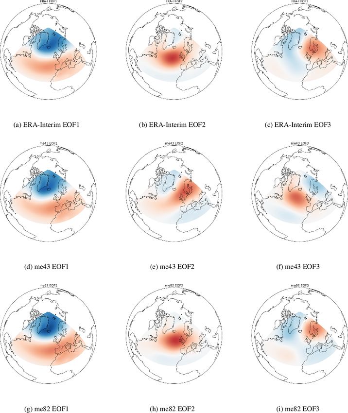
14 E. Gleeson et al.: Extreme Ocean States Northeast Atlantic
Figure 1. (a–c) The three wave model grids as described in Gallagher et al. (2016a). (a) The large North Atlantic grid has a 0.75◦ × 0.75◦
resolution. (b) The grid for the Northeast Atlantic has a 0.25◦ × 0.25◦ resolution. Right panel (c) The wave model unstructured grid around
Ireland has a resolution ranging from 15 km offshore to 1 km in the nearshore characterised by 4473 nodes.
each year in the 30-year periods (i.e. gridded files containing data and a historical WAVEWATCH III simulation driven
120 months of MSLP data). by ERA-Interim fields. The biases are mostly within 10 %.
We used the Python eof library to calculate the EOFs and The EC-Earth ensemble of projections suggests decreases
PCs using the EC-Earth MSLP data where the EOFs are of up to 14 % in the 95th percentile of 10 m wind speed
expressed as a covariance between the PC time series and over the North Atlantic by the end of the century for win-
the MSLP anomalies at each grid point. The MSLP anoma- ter (DJF) under RCP8.5. In accordance, WAVEWATCH III
lies were computed using the 1864–1963 base period (NAO, suggests decreases in the 95th percentile of Hs of 5 %–10 %
2018) of the relevant EC-Earth historical ensemble member. around Ireland by the end of the century. Further details on
The same base period as in Gleeson et al. (2017) was used the evaluation of the winds from EC-Earth and the winds
for consistency. and waves from WAVEWATCH III are available in Gallagher
Individual EOFs sometimes have a physical interpretation et al. (2016a) and Gleeson et al. (2017).
associated with them. In terms of MSLP in the Atlantic re- In the following subsections we analyse the relationships
gion, the first EOF refers to the NAO. The second and third between the 95th percentile of Hs and the PC time series as-
EOFs refer to the EA or the SCAND patterns. In our calcula- sociated with the NAO, EA and SCAND teleconnection pat-
tions the NAO accounted for 35 %–46 % of the MSLP vari- terns for the historical period 1980–2009 and the future pe-
ability, the EA accounted for 15 %–20 % and the SCAND riod 2070–2099 under both RCP4.5 and RCP8.5 forcing sce-
accounted for 10 %–15 %. narios. Spearman correlations are presented in Sect. 4.1 and
Sample EOF maps for the ERA-Interim dataset are shown 20-year return levels of Hs for different combinations of the
in Fig. 2a to c. me43 and me82 are shown in Fig. 2d to f NAO, EA and SCAND indices using extreme value theory
and g to i respectively. Note that the EOF2 of me43 cor- are discussed in Sect. 4.2. 20 years return levels were used,
responds to the SCAND pattern and EOF3 corresponds to following on from previous work by Gleeson et al. (2017).
the EA pattern and that the positive centre of the EA has a Other return periods can, of course, be calculated with the
more northwesterly position than in ERA-Interim or me82. fitted model parameters.
For some of the ensemble members it was more difficult
to determine whether EOF2/3 corresponded to the EA or
4.1 Correlations between the NAO, EA and SCAND and
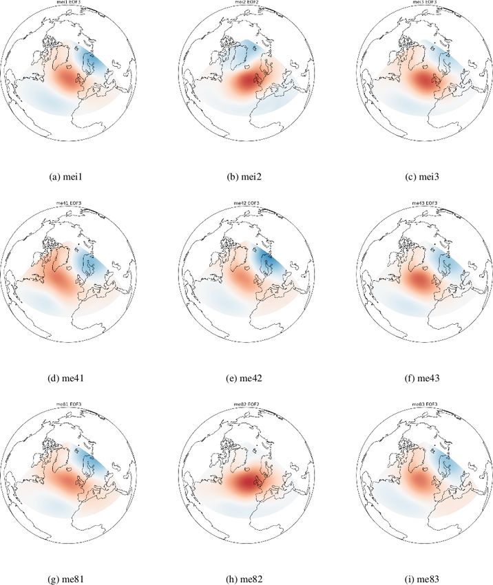
SCAND pattern. Figures A1 and A2 in the Appendix show
the 95th percentile of Hs
the EA and SCAND patterns respectively for each historical,
RCP4.5 and RCP8.5 ensemble member. As in Gleeson et al. (2017), but with minor differences, the
95th percentile of Hs is positively correlated with the PC
4 Analysis and results time-series associated with the NAO, with large areas west
of Ireland where it exceeds +0.7. Figures 3 and 4 show the
We evaluated means and extremes of the EC-Earth 10 m Spearman correlation coefficient between the PC time-series
wind speeds using the ERA-Interim dataset, and the WAVE- corresponding to the EA and the SCAND respectively and
WATCH III outputs using buoy observations, scatterometer the 95th percentile of Hs for the months of December to
Adv. Sci. Res., 16, 11–29, 2019 www.adv-sci-res.net/16/11/2019/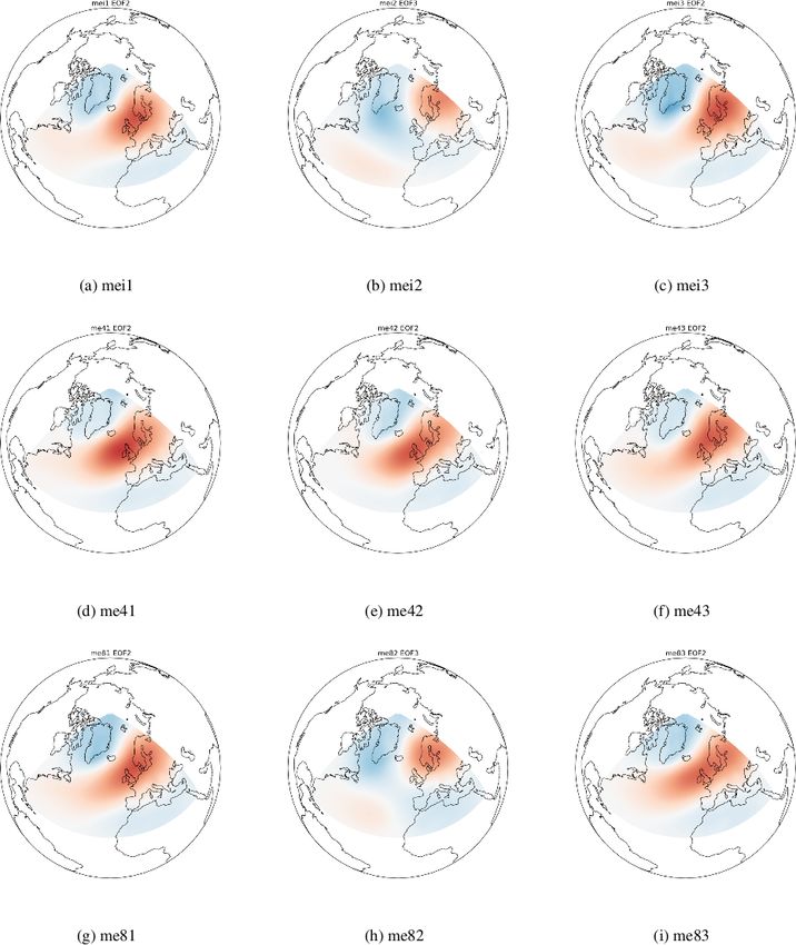
E. Gleeson et al.: Extreme Ocean States Northeast Atlantic                                                                           15

Figure 2. The first three EOF patterns for ERA-Interim (a) to (c), EC-Earth me43 (d) to (f) and EC-Earth me82 (g) to (i).

March. In Figs. 3 and 4 the results shown in (a)–(c) are for the        south of the country, correlations are negative. This is con-
historical period and show each of the 3 ensemble members,              sistent with the fact that EA in its negative phase is associ-
(d)–(f) are for the future period under RCP4.5 and similarly            ated with a centre of low pressure in the North Atlantic west
(g)–(i) are for the future period under RCP8.5. Correlations            of Ireland and hence larger waves. Correlations of both sign
which are statistically significant at the 0.05 level are dotted.       increase further away from Ireland. Correlations are mostly
   In Fig. 3 areas to the north of Ireland tend to mostly show          statistically not significant around the north coast of Ireland.
a positive correlation between the PC corresponding to the                 Again in Fig. 4 the statistically significant correlations at
EA and 95th percentile of Hs while around Ireland and to the            the 95 % confidence limit are dotted. Correlations are mostly

www.adv-sci-res.net/16/11/2019/                                                                       Adv. Sci. Res., 16, 11–29, 2019
16                                                                E. Gleeson et al.: Extreme Ocean States Northeast Atlantic

Figure 3. The Spearman correlation coefficient between the EA index and the 95th percentile of Hs for DJFM. (a–c) historical period
(1980–2009) 3× ensemble members; (d–f) future period 2070–2099 under RCP4.5 and similarly (g–h) is for 2070–2099 under RCP8.5.
Correlations statistically significant at the α < 0.05 level are dotted.

negative around Ireland and positive further north. This is         percentile of Hs can be clearly seen in Fig. 4b and h where
consistent with the behaviour of the SCAND index. In its            areas of positive correlation extend much further south.
positive phase there is an area of high pressure extending
from Scandinavia towards Europe with an area of low pres-
sure around Greenland. Note that the SCAND pattern for              4.2   The NAO, EA and SCAND teleconnections vs
mei2 and me82 (see Fig. A2) shows the area of low pressure                20-year return levels of Hs
around Greenland extending further south into the Atlantic
than in the other ensemble members. The influence of this           The Generalised Extreme Value (GEV) distribution may be
on the correlations between the PC time-series and the 95th         used to calculate the extremes of a dataset (Coles, 2001). The
                                                                    maxima of blocks of data (for example monthly or annual)

Adv. Sci. Res., 16, 11–29, 2019                                                                www.adv-sci-res.net/16/11/2019/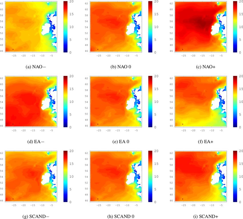
E. Gleeson et al.: Extreme Ocean States Northeast Atlantic 17
may be modelled with the distribution function given by are shown in Fig. C1 in the Appendix. The effect of the NAO
! is clear and robust throughout the datasets; both for the his-
z − µ −1/ξ
torical period and the RCP scenario simulations, return levels
G(z) = exp − 1 + ξ (1)
σ increase significantly when the NAO is positive and are lower
when the NAO is negative or zero. This coincides well with
The three parameters in the distribution are the shape −∞ < the known effects of the NAO in enhancing the westerlies
ξ < ∞, the location −∞ < µ < ∞ and the scale σ > 0. in the North Atlantic and positioning of the jet stream and
Having fitted the parameters to a given dataset, the distri- therefore the storm track, towards the west coast of Ireland.
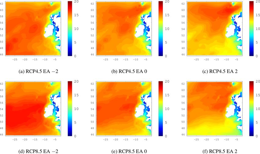
bution function above in Eq. (1) may be inverted to yield N- In comparison to the NAO, the influence of the EA and
year return levels; that is, the value that has a 1/N probability SCAND indices on Hs over our domain is much smaller
of being exceeded in a given year, given by (Fig. 5). Figures C2 and C3 in the Appendix show the cor-
σ responding EA and SCAND 20-year return level plots under
1 − [− log(1 − /N)]−ξ
zN = µ − (2) RCP4.5 and RCP8.5 forcings. When the EA index becomes
ξ
positive, the 20-year return levels of Hs decrease in the south
In this work we applied the GEV to the DJFM monthly of the study domain in particular and the higher wave heights
maxima of the Hs data described above. The model was fit- seem to be “pushed further north”. The decrease in wave
ted with maximum likelihood (ML) inference using the ismev heights south of Ireland is consistent with the centre of posi-
package in R (http://CRAN.R-project.org/package=ismev, tive MSLP anomalies that characterises the EA pattern. The
last access: 18 March 2019). The parameters in the GEV negative effect of a positive-phase EA on 20-year return lev-
are often allowed to be non-stationary. For instance, linear els of Hs is also observed in the RCP simulations.
or harmonic dependence in time may be included to model Figure 5g to i shows the isolated effect of the SCAND pat-
long-term trends or seasonality in extremes; see, for exam- tern on 20-year return levels of Hs by keeping the NAO and
ple, Caires et al. (2006), Clancy et al. (2015), Izaguirre et al. the EA indices set to values of 0. The effect is more diffi-
(2011). In Gleeson et al. (2017), the GEV model was applied cult to see in the ensemble mean of the historical simulations
to the present dataset with station-based NAO used as a co- but is clear in the RCP4.5/8.5 SCAND plots in Fig. C3 in the
variate for the location and scale parameters. Appendix. As mentioned earlier, the SCAND pattern in mei2
In this present work, we allowed the location parameter has the area of low pressure over Greenland extending fur-
to depend on the three PCs: µ(t) = µ0 + µ1 × PC1(t) + µ2 × ther south than in the other 2 ensemble members and makes
PC2(t) + µ3 × PC3(t). The shape and scale parameters were the effect of the SCAND pattern on wave heights more dif-
kept constant, as was the case in Izaguirre et al. (2011). With ficult to see. As the SCAND index goes from a positive to
such a model, we see from Eq. (2) that any overall increase a negative phase, 20-year return levels of Hs decrease in the
(decrease) in µ will result in higher (lower) return levels of southeast of the domain but seem to increase in the north, for
extremes. the historical period as well as for the RCPs. The SCAND is
In all ensemble members for both historical and future sce- associated with easterly winds from a blocking anticyclonic
narios, the ML estimate of µ1 , relating to the NAO (PC1), set-up over Scandinavia and is known to divert the Atlantic
was found to be non-negative throughout the domain. Thus, jet stream east of its climatological position (Bueh and Naka-
a positive phase of the NAO may contribute to an increase in mura, 2007). The physical effects we see here are consistent
extremes of Hs . This effect of the NAO was discussed in de- with the known climatic impacts of the SCAND pattern.
tail in Gleeson et al. (2017), and in particular how this is ex- Ensemble means of the 20-year return levels of Hs are
pected to vary under the two future scenarios. Here we focus shown in Fig. 6 for the historical period and future peri-
on the EA and SCAND. In Figs. B1 and B2 in the Appendix ods under RCP4.5 and RCP8.5 where the NAO index is +2
we show the ML estimates of µ2 and µ3 , respectively. Each and the EA and SCAND indices are set to −2. Of the three
ensemble member is shown for the historical and two future teleconnections, the NAO has the strongest influence on ex-
periods. Note the similarities, as expected, between the cor- treme waves in the northeast Atlantic, followed by the EA
relation maps in Fig. 3 and the spatial distribution of µ2 in with the SCAND having the smallest influence. Figure 6c
Fig. B1 and similarly between Figs. 4 and B2 for the SCAND clearly shows that under RCP8.5 in particular the 20-year re-
and the distribution of µ3 . turn levels of Hs may increase off the west coast of Ireland
The remainder of this section is dedicated to the influence despite a prediction of an overall decreasing trend in mean
of the NAO, EA and SCAND indices on 20-year return levels wind speeds and thus waves.
of Hs . Varying the NAO from −2 to 0 to +2, while keeping
the EA and SCAND in a neutral state of zero, shows a clear
increase in the 20-year return levels of Hs when the NAO is 5 Conclusions
in its positive phase. This is shown in Fig. 5a–c where the
ensemble means of the 3 members for the historical period We analysed principal component time-series associated
are shown. Corresponding results under RCP4.5 and RCP8.5 with the NAO, EA and SCAND teleconnection patterns com-
www.adv-sci-res.net/16/11/2019/ Adv. Sci. Res., 16, 11–29, 2019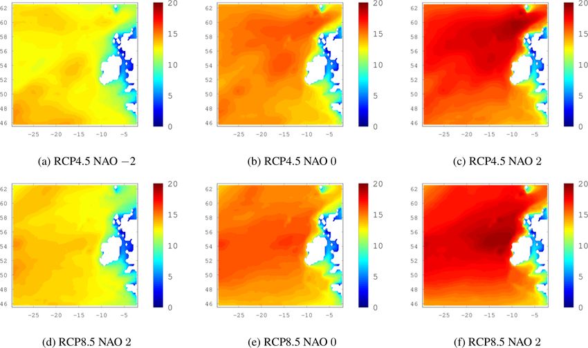
18                                                                 E. Gleeson et al.: Extreme Ocean States Northeast Atlantic

Figure 4. The Spearman correlation coefficient between the SCAND index and the 95th percentile of Hs for DJFM. (a–c) historical period
(1980–2009) 3× ensemble members; (d–f) future period 2070–2099 under RCP4.5 and similarly (g–h) is for 2070–2099 under RCP8.5.
Correlations statistically significant at the α < 0.05 level are dotted.

puted using an ensemble of global EC-Earth climate projec-           High. Stronger westerly winds, associated with the increased
tions and the influence of these patterns on regional wave           pressure gradient, also generate larger waves. The East At-
projections over the North Atlantic. The influence of the            lantic pattern, in its negative phase, has a centre of negative
NAO on extreme waves is greater than that of the EA and              MSLP anomalies over the eastern North Atlantic, roughly be-
SCAND teleconnection patterns. We found that the 20-year             tween the two centres of the NAO. This is also associated
return levels of Hs are largest when the NAO is in a strong          with stronger winds and therefore larger waves. The negative
positive phase (e.g. +2) and the EA and SCAND are in                 phase of the SCAND pattern has a negative pole of MSLP
strong negative phases (e.g. −2). During the positive phase          anomalies centered over Scandinavia. When the NAO is in
of the NAO the pressure gradient over the North Atlantic in-         a positive phase, the SCAND pattern enhances the westerly
creases due to strengthening of the Icelandic Low and Azores         winds over the Atlantic which in turn has a positive impact

Adv. Sci. Res., 16, 11–29, 2019                                                                  www.adv-sci-res.net/16/11/2019/
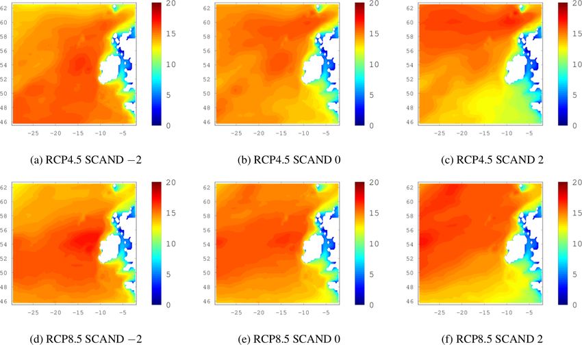
E. Gleeson et al.: Extreme Ocean States Northeast Atlantic                                                                             19

Figure 5. 20-year return levels of Hs where the effects of the NAO, EA and SCAND are isolated by setting each of the remaining two indices
to zero. The ensemble mean is shown for the historical simulations.

Figure 6. Ensemble mean 20-year return levels of Hs where the NAO is set to +2 and both the EA and SCAND are −2. A positive phase
NAO and negative phase EA and SCAND is associated with the highest waves off Ireland.

www.adv-sci-res.net/16/11/2019/                                                                      Adv. Sci. Res., 16, 11–29, 2019
20                                                                   E. Gleeson et al.: Extreme Ocean States Northeast Atlantic

on wave heights off the west coast of Ireland. This is why
the +, −, − patterns for the NAO, EA and SCAND respec-
tively are assoicated with the largest significant wave heights
as found in this study. Gleeson et al. (2017) showed that local
increases in extreme waves are possible in the future under
RCP8.5. The results presented here are consistent with this
but also include the effects of the EA and SCAND whose
centres of action modulate the influence of the NAO on Hs.
   The running of CMIP6 climate simulations is currently in
progress and we plan to repeat the analysis by carrying out
new multi-model global climate simulations and downscaled
simulations. It is also worth noting that the second and third
EOF patterns vary quite a lot. Having a larger ensemble size
would be of benefit and would make the results more ro-
bust. In addition, we used two 30-year periods 1980–2009
and 2070–2099. The analysis would also benefit from using
rolling 30-year periods. In addition we are currently doing a
separate analysis of the wave energy flux and wave period.
   Although climate projections suggest that Hs and wave en-
ergy flux will decrease on average in the Northeast Atlantic
Ocean by the end of the century, extremes will still occur
and may be enhanced depending on the phase of large-scale
patterns such as the NAO, EA and SCAND.

Data availability. The datasets have been archived at Met Éireann.
There is currently no publicly available method for data access so
the Met Éireann should be contacted for dataset access.

Adv. Sci. Res., 16, 11–29, 2019                                                               www.adv-sci-res.net/16/11/2019/
E. Gleeson et al.: Extreme Ocean States Northeast Atlantic                                        21

Appendix A: EA and SCAND Patterns

Figure A1. EOF patterns (2 or 3) corresponding to the EA telecon-
nection for the EC-Earth historical and future periods under RCP4.5
and RCP8.5.

www.adv-sci-res.net/16/11/2019/                                       Adv. Sci. Res., 16, 11–29, 2019
22                                                                    E. Gleeson et al.: Extreme Ocean States Northeast Atlantic

Figure A2. EOF patterns (2 or 3) corresponding to the SCAND
teleconnection for the EC-Earth historical and future periods under
RCP4.5 and RCP8.5.

Adv. Sci. Res., 16, 11–29, 2019                                                                www.adv-sci-res.net/16/11/2019/
E. Gleeson et al.: Extreme Ocean States Northeast Atlantic                                           23

Appendix B: Maximum likelihood estimate of the µ2
and µ3 parameters

Figure B1. Maximum likelihood estimate of the µ2 parameter. The
three ensemble members are shown for the historical period (a)
to (c), future period under RCP4.5 (d) to (f), and future period under
RCP8.5 (g) to (i).

www.adv-sci-res.net/16/11/2019/                                          Adv. Sci. Res., 16, 11–29, 2019
24                                                                       E. Gleeson et al.: Extreme Ocean States Northeast Atlantic

Figure B2. Maximum likelihood estimate of the µ3 parameter. The
three ensemble members are shown for the historical period (a)
to (c), future period under RCP4.5 (d) to (f), and future period under
RCP8.5 (g) to (i).

Adv. Sci. Res., 16, 11–29, 2019                                                                   www.adv-sci-res.net/16/11/2019/
E. Gleeson et al.: Extreme Ocean States Northeast Atlantic                                        25

Appendix C: 20-year return levels of Hs for varying
values of the NAO, EA and SCAND indices

Figure C1. 20-year return levels of Hs . The NAO index varies from
3 values of the NAO index while the EA and SCAND are held in
their neutral state (zero). The top row shows the ensemble mean for
the future period under RCP4.5 and the bottom row is similar but
shows RCP8.5 results.

www.adv-sci-res.net/16/11/2019/                                       Adv. Sci. Res., 16, 11–29, 2019
26                                                                    E. Gleeson et al.: Extreme Ocean States Northeast Atlantic

Figure C2. 20-year return levels of Hs . The EA index varies from
3 values of the NAO index while the NAO and SCAND are held in
their neutral state (zero). The top row shows the ensemble mean for
the future period under RCP4.5 and the bottom row is similar but
shows RCP8.5 results.

Adv. Sci. Res., 16, 11–29, 2019                                                                www.adv-sci-res.net/16/11/2019/
E. Gleeson et al.: Extreme Ocean States Northeast Atlantic                                        27

Figure C3. 20-year return levels of Hs . The SCAND index varies
from 3 values of the NAO index while the NAO and EA are held in
their neutral state (zero). The top row shows the ensemble mean for
the future period under RCP4.5 and the bottom row is similar but
shows RCP8.5 results.

www.adv-sci-res.net/16/11/2019/                                       Adv. Sci. Res., 16, 11–29, 2019
28                                                                      E. Gleeson et al.: Extreme Ocean States Northeast Atlantic

Author contributions. EG ran the EC-Earth global climate simu-           Caires, S., Swail, V. R., and Wang, X. L.: Projection and analysis of
lations, analysed the wind outputs and computed the PC time-series          extreme wave climate, J. Climate, 19, 5581–5605, 2006.
using EC-Earth data; SG ran the WAVEWATCH III simulations us-            Charles, E., Idier, D., Thiébot, J., Le Cozannet, G., Pedreros, R.,
ing EC-Earth boundary conditions, JJ analysed the wave outputs              Ardhuin, F., and Planton, S.: Present Wave Climate in the Bay
and correlations between significant wave height and the PC time-           if Biscay: Spatiotemporal Variability and Trends from 1958 to
series; CC did a statistical analysis of extreme waves and the PC           2001, J. Climate, 25, 2020–2039, 2012.
time-series using a Generalised Extreme Value distribution. EG, CC       Clancy, C., Belissen V, Tiron, R., Gallagher, S., and Dias, F.: Spatial
and LZ analysed the outputs of the statistical tests. EG and CC pre-        variability of extreme sea states on the Irish west coast, in: Pro-
pared the manuscript and received contributions from JJ, LZ, FD             ceedings of the ASME 2015 34th International Conference on
and SG.                                                                     Ocean, Offshore and Arctic Engineering, St John’s, NL, Canada,
                                                                            2015.
                                                                         Coles, S.: An introduction to statistical modeling of extreme values,
Competing interests. The authors declare that they have no con-             Springer-Verlag London, 2001.
flict of interest.                                                       Comas-Bru, L. and McDermott, F.: Impacts of the EA and SCA
                                                                            patterns on the European twentieth century NAO-winter cli-
                                                                            mate relationship, Q. J. Roy. Meteor. Soc., 140, 354–363,
Special issue statement. This article is part of the special issue          https://doi.org/10.1002/qj.2158, 2014.
“18th EMS Annual Meeting: European Conference for Applied Me-            Dodet, G., Bertin, X., and Taborda, R.: Wave climate variability in
teorology and Climatology 2018”. It is a result of the EMS Annual           the North-East Atlantic Ocean over the last six decades, Ocean
Meeting: European Conference for Applied Meteorology and Cli-               Model., 31, 120–131, 2010.
matology 2018, Budapest, Hungary, 3–7 September 2018.                    Fichefet, T. and Maqueda, M.: Sensitivity of a global sea ice model
                                                                            to the treatment of ice thermodynamics and dynamics, J. Geo-
                                                                            phys. Res.-Oceans, 102, 12609–12646, 1997.
                                                                         Gallagher, S., Tiron, R., and Dias, F.: A detailed investigation of
Acknowledgements. The authors wish to acknowledge Rox-
                                                                            the nearshore wave climate and the nearshore wave energy re-
ana Tiron who helped to run the wave simulations and the EC-Earth
                                                                            source on the west coast of Ireland, in: Proceedings of the ASME
community for useful discussions on principal component analysis
                                                                            2013 32nd International Conference on Ocean, Offshore and
outputs. The numerical simulations were performed on the Fionn
                                                                            Arctic Engineering OMAE, American Society of Mechanical
cluster at the Irish Centre for High-end Computing (ICHEC) and
                                                                            Engineers, Nantes, France, https://doi.org/10.1115/OMAE2013-
at the Swiss National Computing Centre under the PRACE-2IP
                                                                            10719, 2013.
project (FP7 RI-283493) “Nearshore wave climate analysis of the
                                                                         Gallagher, S., Tiron, R., and Dias, F.: A long-term nearshore wave
west coast of Ireland”. The authors would like to thank the review-
                                                                            hindcast for Ireland: Atlantic and Irish Sea coasts (1979–2012),
ers for their useful comments and feedback.
                                                                            Ocean Dynam., 64, 1163–1180, https://doi.org/10.1007/s10236-
                                                                            014-0728-3, 2014.
                                                                         Gallagher, S., Gleeson, E., Tiron, R., McGrath, R., and Dias,
Review statement. This paper was edited by Sandro Carniel and               F.: Wave climate projections for Ireland for the end of
reviewed by Angela Pomaro and one anonymous referee.                        the 21st century including analysis of EC-Earth winds over
                                                                            the North Atlantic Ocean, Int. J. Climatol., 36, 4592–4607,
                                                                            https://doi.org/10.1002/joc.4656, 2016a.
                                                                         Gallagher, S., Tiron, R., Whelan, E., Gleeson, E., Dias,
References                                                                  F., and McGrath, R.: The nearshore wind and wave en-
                                                                            ergy potential of Ireland: A high resolution assessment of
Ardhuin, F., Rogers, E., Babanin, A. V., Filipot, J.-F., Magne, R.,         availability and accessibility, Renew. Energ., 88, 494–516,
  Roland, A., van der Westhuysen, A., Queffeulou, P., Lefevre,              https://doi.org/10.1016/j.renene.2015.11.010, 2016b.
  J.-M., Aouf, L., and Collard, F.: Semiempirical Dissipation            Gleeson, E., McGrath, R., and Treanor, M.: Ireland’s climate: the
  Source Functions for Ocean Waves. Part I: Definition, Cal-                road ahead, Met Éireann, Dublin, Ireland, 2013.
  ibration, and Validation, J. Phys. Oceanogr., 40, 1917–1941,           Gleeson, E., Gallagher, S., Clancy, C., and Dias, F.: NAO and ex-
  https://doi.org/10.1175/2010JPO4324.1, 2010.                              treme ocean states in the Northeast Atlantic Ocean, Adv. Sci.
Atan, R., Goggins, J., and Nash, S.: A Detailed Assessment of the           Res., 14, 23–33, https://doi.org/10.5194/asr-14-23-2017, 2017.
  Wave Energy Resource at the Atlantic Marine Energy Test Site,          Greatbatch, R. J.: The North Atlantic Oscillation, Stoch. Env. Res.
  Energies, 9, 967, https://doi.org/10.3390/en9110967, 2016.                Risk A., 14, 213–242, 2000.
Barnston, A. and Livezey, E.: Classification, seasonality and persis-    Hazeleger, W., Severijns, C., Semmler, T., Ştefănescu, S., Yang,
  tence of low-frequency atmospheric circulation patterns, Mon.             S., Wang, X., Wyser, K., Dutra, E., Baldasano, J., Bintanja,
  Weather Rev., 115, 1083–1126, 1987.                                       R., Bougeault, P., Caballero, R., Ekman, A. M. L., Chris-
Bertin, X., Prouteau, E., and Letetrel, C.: A significant increase in       tensen, J. H., van den Hurk, B., Jimenez, P., Jones, C., Kåll-
  waveheight in the North Atlantic Ocean over the 29th century,             berg, P., Koenigk, T., McGrath, R., Miranda, P., Van Noije,
  Global Planet. Change, 106, 77–83, 2013.                                  T., Palmer, T., Parodi, J., Schmith, T., Selten, F., Storelvmo,
Bueh, C. and Nakamura, H.: Scandinavian pattern and its cli-                T., Sterl, A., Tapamo, H., Vancoppenolle, M., Viterbo, P., and
  matic impact, Q. J. Roy. Meteor. Soc., 133, 2117–2131,                    Willén, U.: EC-Earth: A Seamless Earth-System Prediction
  https://doi.org/10.1002/qj.173, 2007.

Adv. Sci. Res., 16, 11–29, 2019                                                                        www.adv-sci-res.net/16/11/2019/
E. Gleeson et al.: Extreme Ocean States Northeast Atlantic 29 Approach in Action, B. Am. Meteor. Soc., 91, 1357–1363, Scherrer, S. C., Croci-Maspoli, M., Schwierz, C., and Appenzeller, https://doi.org/10.1175/2010BAMS2877.1, 2010. C.: Two-dimensional indices of atmospheric blocking and their Hazeleger, W., Wang, X., Severijns, C., Ştefănescu, S., Bintanja, statistical relationship with winter climate patterns in the Euro- R., Sterl, A., Wyser, K., Semmler, T., Yang, S., van den Hurk, Atlantic region, Int. J. Climatol., 26, 233–250, 2006. B., van Noije, T., van der Linden, E., and van der Wiel, K.: Taylor, K. E., Stouffer, R. J., and Meehl, G. A.: An overview of EC-Earth V2.2: description and validation of a new seamless CMIP5 and the experiment design, B. Am. Meteor. Soc., 93, earth system prediction model, Clim. Dynam., 39, 2611–2629, 485–498, 2012. https://doi.org/10.1007/s00382-011-1228-5, 2012. Tolman, H.: User manual and system documentation of Wavewatch Hurrell, J.: Decadal trends in the North Atlantic Oscillation: re- III version 4.18, Tech. Rep. 316, NOAA/NWS/NCEP/MMAB, gional temperatures and precipitation, Oceanographic Literature 2014. Review, 2, 116, https://doi.org/10.1126/science.269.5224.676, Trigo, R. M., Valente, M. A., Trigo, I. F., Miranda, P. M. A., Ramos, 1996. A. M., Paredes, D., and García-Herrera, R.: The Impact of North Izaguirre, C., Mendez, F. J., Menendez, M., Luceño, A., and Atlantic Wind and Cyclone Trends on European Precipitation Losada, I. J.: Extreme wave climate variability in southern and Significant Wave Height in the Atlantic, Ann. NY Acad. Sci., Europe using satellite data, J. Geophys. Res.-Oceans, 115, 1146, 212–234, https://doi.org/10.1196/annals.1446.014, 2008. https://doi.org/10.1029/2009JC005802, 2010. Valcke, S.: OASIS3 user guide (prism_2-5), PRISM support initia- Izaguirre, C., Méndez, F. J., Menéndez, M., and Losada, I. J.: Global tive report, 3, 64, 2006. extreme wave height variability based on satellite data, Geophys. van Loon, H. and Rogers, J. C.: The seesaw in winter temperatures Res. Lett., 38, 1–6, 2011. between Greenland and northern Europe. Part I: General descrip- Janssen, P. A.: Progress in ocean wave forecasting, J. Comput. tion, Mon. Weather Rev., 106, 296–310, 1978. Phys., 227, 3572–3594, 2008. Vautard, R.: Multiple Weather Regimes over the North At- Komen, G. J., Cavaleri, L., Donelan, M., Hasselmann, K., Hassel- lantic: Analysis of Precursors and Successors, Mon. mann, S., and Janssen, P.: Dynamics and modelling of ocean Weather Rev., 118, 2056–2081, https://doi.org/10.1175/1520- waves, Cambridge university press, 1994. 0493(1990)1182.0.CO;2, 1990. Madec, G.: Nemo ocean engine: Note du pole de modélisation, Wallace, J. M. and Gutzler, D. S.: Teleconnections in the Geopo- Institut Pierre-Simon Laplace (IPSL), France, No 27 ISSN No tential Height Field during the Northern Hemisphere Winter, 1288–1619, 2008. Mon. Weather Rev., 109, 784–812, https://doi.org/10.1175/1520- NAO: The Climate Data Guide: Hurrell North At- 0493(1981)1092.0.CO;2, 1981. lantic Oscillation (NAO) Index (station-based), avail- Wang, X. and Swail, V.: Changes of extreme wave heights in able at: https://climatedataguide.ucar.edu/climate-data/ Northern Hemisphere oceans and related atmospheric circulation hurrell-north-atlantic-oscillation-nao-index-station-based, regimes, J. Climate, 14, 2204–2221, 2001. last acces: 28 November 2018. Wang, X. and Swail, V.: Trends of Atlantic wave extremes as simu- Pokorná, L. and Huth, R.: Climate impacts of the NAO are sensitive lated in a 40-year wave hindcast using kinematically reanalysed to how the NAO is defined, Theor. Appl. Climatol., 119, 639– wind fields, J. Climate, 15, 1020–1035, 2002. 652, 2015. Woollings, T. and Blackburn, M.: The North Atlantic Jet Stream Roland, A.: Development of WWM II: Spectral wave modelling under Climate Change and Its Relation to the NAO and EA Pat- on unstructured meshes, PhD thesis, Institute of Hydraulics and terns, J. Climate, 25, 886–902, https://doi.org/10.1175/JCLI-D- Wave Resource Engineering, Technical University Darmstadt, 11-00087.1, 2012. Germany, 2008. Zubiate, L., McDermott, F., Sweeney, C., and O’Malley, M.: Spa- Santo, H., Taylor, P., Taylor, R. E., and Stansby, P.: Decadal vari- tial variability in winter NAO-wind speed relationships in west- ability of wave power production in the North-East Atlantic and ern Europe linked to concomitant states of the East Atlantic and North Sea for the M4 machine, Renew. Energ., 91, 442–450, Scandinavian patterns, Q. J. Roy. Meteor. Soc., 143, 552–562, https://doi.org/10.1016/j.renene.2016.01.086, 2016a. https://doi.org/10.1002/qj.2943, 2017. Santo, H., Taylor, P. H., and Gibson, R.: Decadal variability of ex- treme wave height representing storm severity in the northeast Atlantic and North Sea since the foundation of the Royal So- ciety, P. R. Soc. A, 472, https://doi.org/10.1098/rspa.2016.0376, 2016b. www.adv-sci-res.net/16/11/2019/ Adv. Sci. Res., 16, 11–29, 2019
You can also read