Robust Arctic warming caused by projected Antarctic sea ice loss
←
→
Page content transcription
If your browser does not render page correctly, please read the page content below
Environmental Research Letters

LETTER • OPEN ACCESS

Robust Arctic warming caused by projected Antarctic sea ice loss
To cite this article: M R England et al 2020 Environ. Res. Lett. 15 104005

View the article online for updates and enhancements.

                                This content was downloaded from IP address 176.9.8.24 on 26/09/2020 at 04:43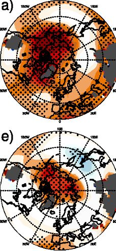
Environ. Res. Lett. 15 (2020) 104005 https://doi.org/10.1088/1748-9326/abaada
Environmental Research Letters
LETTER
Robust Arctic warming caused by projected Antarctic sea ice loss
OPEN ACCESS
M R England1,2, L M Polvani3,4 and L Sun5
RECEIVED 1
14 May 2020 Department of Climate, Atmospheric Science and Physical Oceanography, Scripps Institution of Oceanography, La Jolla, CA, United
States of America
REVISED 2
28 July 2020
Department of Physics and Physical Oceanography, University of North Carolina Wilmington, NC, United States of America
3
Department of Applied Mathematics and Applied Physics, Columbia University, New York, NY, United States of America
ACCEPTED FOR PUBLICATION 4
Department of Earth and Environmental Science, Lamont Doherty Earth Observatory, Columbia University, Palisades, NY, United
30 July 2020
States of America
5
PUBLISHED Department of Atmospheric Science, Colorado State University, Fort Collins, CO, United States of America
17 September 2020
Keywords: sea ice loss, polar climate change, arctic, antarctic, climate model simulations, climate projections
Original Content from Supplementary material for this article is available online
this work may be used
under the terms of the
Creative Commons
Attribution 4.0 licence.
Abstract
Any further distribution
of this work must Over the coming century, both Arctic and Antarctic sea ice cover are projected to substantially
maintain attribution to
the author(s) and the title
decline. While many studies have documented the potential impacts of projected Arctic sea ice loss
of the work, journal on the climate of the mid-latitudes and the tropics, little attention has been paid to the impacts of
citation and DOI.
Antarctic sea ice loss. Here, using comprehensive climate model simulations, we show that the
effects of end-of-the-century projected Antarctic sea ice loss extend much further than the tropics,
and are able to produce considerable impacts on Arctic climate. Specifically, our model indicates
that the Arctic surface will warm by 1 ◦ C and Arctic sea ice extent will decline by 0.5 × 10⁶ km2 in
response to future Antarctic sea ice loss. Furthermore, with the aid of additional atmosphere-only
simulations, we show that this pole-to-pole effect is mediated by the response of the tropical SSTs
to Antarctic sea ice loss: these simulations reveal that Rossby waves originating in the tropical
Pacific cause the Aleutian Low to deepen in the boreal winter, bringing warm air into the Arctic,
and leading to sea ice loss in the Bering Sea. This pole-to-pole signal highlights the importance of
understanding the climate impacts of the projected sea ice loss in the Antarctic, which could be as
important as those associated with projected sea ice loss in the Arctic.
1. Introduction and Simmonds 2010, Screen et al 2013, England et al
2018). Sea ice loss also has an important impact on
The Arctic has lost over 40% of its summer sea the mid-latitude tropospheric jet, with Arctic sea ice
ice extent over the past forty years (see, e.g. the loss causing an equatorward shift of the Northern
NSIDC Sea Ice Index, Fetterer et al 2017). Meanwhile, Hemisphere mid-latitude jet (Peings and Magnusdot-
Antarctic sea ice extent has fallen to record lows over tir 2014, Screen et al 2018), and Antarctic sea ice
the past four years after a 35-year period of small loss causing a weakening of the Southern Hemisphere
but significant sea ice growth (Parkinson 2019). More mid-latitude jet (England et al 2018, Ayres and Screen
importantly, by the end of this century, climate mod- 2019). In fact, several studies with coupled ocean-
els project that both Arctic and the Antarctic sea ice atmosphere models have suggested that the response
covers will shrink considerably (Collins et al 2006, to sea ice loss can be global in nature (Deser et al 2015,
Notz et al 2020), and a welter of studies have focused Deser et al 2016, Screen et al 2018, Sun et al 2020).
on determining if and how the projected sea ice loss at Specifically, the effects of sea ice loss have been shown
the poles could impact the climate system at lower lat- to extend to the tropics (Wang et al 2018, England
itudes (Shepherd 2016, Screen 2017, Screen et al 2018, et al 2020, Kennel and Yulaeva 2020), with enhanced
Cohen et al 2020). warming and precipitation in the equatorial regions,
Observational and modeling evidence has shown and even reaching deep into the opposite hemisphere
that sea ice loss causes a robust warming and moisten- (Deser et al 2015, Liu and Fedorov 2018). A detailed
ing of the atmosphere at the high-latitudes, especially examination of the pole-to-pole effects of projected
in the lower troposphere (Deser et al 2010, Screen sea ice loss, however, is still lacking.
© 2020 The Author(s). Published by IOP Publishing Ltd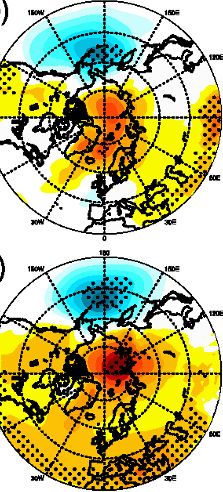
Environ. Res. Lett. 15 (2020) 104005                                                                M England et al

     And yet, from a paleoclimatic perspective the        start by detailing the model we use and the simula-
idea that the polar regions may be connected is           tions we analyze, then present the results, and con-
not new. Evidence from ice cores from the last gla-       clude with a brief discussion.
cial and deglacial period indicates that past peri-
ods of warming in the northern high-latitudes coin-       2. Methods
cided with periods of cooling in the southern high-
latitudes, and vice versa (Blunier et al 1998, Blunier    2.1. Model
and Brook 2001, Barbante et al 2006, Pedro et al          In this study we analyze climate model simulation
2011): this phenomenon, whereby temperature at the        performed with the Community Earth System Model
poles are at opposite phases on millennial timescales,    (CESM1) Whole Atmosphere Coupled Chemistry
is known as the ‘bipolar seesaw’ hypothesis (Broecker     Model (WACCM4). CESM1-WACCM4 is fully doc-
1998, Marino et al 2015, Pedro et al 2018). Most          umented in Marsh et al (2013), to which the reader is
studies have pointed to the deep ocean circulation        referred to for details. The atmospheric component,
as the likely mediator of this anti-correlated beha-      WACCM4, has a horizontal resolution of 1.9◦ latit-
vior of the climate at the two poles (Crowley 1992,       ude by 2.5◦ longitude, with 66 vertical levels and a
Stocker 1998, Stocker and Johnsen 2003, Knutti et al      model top in the lower thermosphere. The represent-
2004). Recently it has been suggested that the ‘bipolar   ation of the stratospheric chemistry and dymamics
seesaw’ mechanism might operate on much shorter—          in WACCM4 is much superior to the one in typ-
multi-decadal—timescales, and that this may be seen       ical low-top models, owing to improved vertical res-
in the observed temperature record from the last cen-     olution, gravity wave parameterisation for the upper
tury (Chylek et al 2010, Wang et al 2015). It seems,      atmosphere, and interactive stratospheric chemistry.
however, that this phenomenon is likely an artifact       This is important because previous studies have iden-
of the limited Antarctic data coverage (Schneider and     tified the stratosphere as a potential pathway for polar
Noone 2012). In any case, most of the literature on       sea ice loss to influence the lower latitudes (Sun et al
pole-to-pole linkages is focused on the two polar         2015, Zhang et al 2018, De and Wu 2019). The atmo-
regions behaving asynchronously.                          spheric component is coupled to land, ocean and sea
     More recently, a handful of modeling studies have    ice components, making CESM1-WACCM4 a CMIP-
suggested that future Arctic sea ice loss can poten-      class fully-coupled climate system model.
tially impact the climate of Antarctica. Notably, Liu
and Fedorov (2018) have reported that in the first        2.2. Fully-coupled runs
fifteen years following a large, abrupt loss of Arctic    To understand the climate response to projected Ant-
sea ice, the southern high-latitudes cool and Antarc-     arctic sea ice loss we analyze two simulations with per-
tic sea ice cover expands (via an atmospheric con-        turbed sea ice cover, described detail in England et al
nection), in a manner reminiscent of the ‘bipolar         (2020). Both are 350-year long, time-slice integra-
seesaw’; however, unlike the initial transient phase,     tions of the fully-coupled CESM1-WACCM4 model,
the equilibrium response to Arctic sea ice loss in the    with all anthropogenic forcings fixed at year 1955 val-
same model simulations features a clear warming of        ues. These include CO2 , methane, nitrous oxide and,
the southern high-latitudes. Such Antarctic warming       most importantly, ozone depleting substances (which
is consistent with the results of Deser et al (2015),     may have contributed to the recent warming in the
who show that projected Arctic sea ice loss leads         Arctic, as reported in Polvani et al 2020). The mid-
to upper-tropospheric warming in the tropics and          twentieth century was chosen as the control period so
lower-tropospheric warming at both poles (termed          as to avoid the impacts of stratospheric ozone deple-
a ‘mini global warming’, due to its resemblance to        tion; stratospheric ozone concentrations are severely
the atmospheric warming pattern caused by increased       perturbed at present (WMO 2018), but are expected
green-house gases). The potential influence in the        to return to pre-1960 values in the second half of this
other direction, however, remains unexplored.             century. We discard the first 100-years of these integ-
     Hence the goal of our paper: to investigate cli-     rations, and focus on the average of the remaining
mate change in the Arctic caused by projected end-        250-years.
of-the-century sea ice loss in the Antarctic. Analyz-         The only difference between these two
ing model integrations specifically designed for this     integrations is their Antarctic sea ice cover.
purpose, we here demonstrate that Antarctic sea ice       In the ‘control’ run Antarctic sea ice condi-
loss also causes a ‘mini global warming’ signal, with     tions are nudged to match the mean of a six-
enhanced warming over the Arctic and a signific-          member ensemble CESM1-WACCM4 historical
ant reduction in Arctic sea ice cover. To understand      runs, averaged over the period 1955-69 (figure
the underlying mechanism, we perform atmosphere-          S1a(https://stacks.iop.org/ERL/15/104005/mmedia)).
only runs, and show that the tropical SST anomalies       In the ‘future’ run Antarctic sea ice conditions are
caused by projected Antarctic sea ice loss drive a sub-   nudged to match the mean of a three-member
stantial portion of the enhanced Arctic warming, via      ensemble of CESM1-WACCM4 RCP8.5 scenario
a Rossby wave trains and a deeper Aleutian Low. We        simulations, averaged over the period 2085-2099

                                             2
Environ. Res. Lett. 15 (2020) 104005 M England et al
(figure S1b). In both cases, Antarctic sea ice con- the Arctic. In our simulations, the Arctic polar cap
ditions are constrained following the methodology (60-90◦ N) surface warms by approximately 1 ◦ C in
of Deser et al (2015), which consists of adding an response to Antarctic sea ice loss. This is a substantial
additional ‘ghost flux’ to the sea ice component of effect, as it accounts for 10–15% of the projected end-
CESM1-WACCM4 so as to maintain the desired sea of-century Arctic warming of 7.5 ◦ C under RCP8.5.
ice concentrations. This approach does not conserve Viewed another way, although this signal has traveled
energy but it does conserve the fresh water budget, all the way from the southern high-latitudes to the
and has been found to be more effective than the northern high-latitudes, it is still 20% as large as the
commonly-used albedo-reduction method (Sun et al 5 ◦ C Antarctic polar cap (60–90◦ S) surface warming,
2020). A detailed explanation can be found in Eng- and twice as large as the 0.5 ◦ C tropical (25◦ S–25◦ N)
land et al (2020). surface warming.
The difference in sea ice concentrations between This results in an Arctic amplification factor,
the control and future runs is shown in figure S1c, and which we define here as the ratio of the Arctic (60–
corresponds to reduction in Antarctic sea ice extent of 90◦ N) warming to tropical (25◦ S–25◦ N) warming,
6.6 × 10⁶ km2 . In the remainder of the paper, we will of 2.2. We note that this is not statistically differ-
refer to the difference between these two runs, aver- ent from the Arctic amplification factor of 2.1 under
aged over the last 250 years, as ‘the response’ to Ant- projected changes under RCP8.5 for this model, as
arctic sea ice loss. determined from the difference between the period
2085–2099 for the RCP8.5 simulations and the period
2.3. Atmosphere-only runs with prescribed 1955–69 for the historical transient simulations. We
tropical SSTs note that the warming under RCP8.5 would include
To investigate the role of tropical SST anomalies in the effects of projected Antarctic sea ice loss. This
driving Arctic warming, we carry out two additional could suggest that this Arctic warming is part of the
model integrations. The first is a 251-year-long ‘con- ‘mini global warming’ response, where local feed-
trol’ run with WACCM4 in atmosphere-only config- backs are the dominant processes in Arctic amplific-
uration, i.e. with sea ice and SSTs prescribed from ation (Stuecker et al 2018). However, in section 3.2,
the climatology (with a monthly-mean repeating sea- we show that a sizable fraction of the Arctic warming
sonal cycle) of the six-member mean of the CESM1- response to projected Antarctic sea ice loss is actually
WACCM4 historical runs, averaged over the period driven remotely from the lower latitudes.
1955-69, and with radiatively active gases fixed at year Zooming into the Arctic, one sees that the ampli-
1955 levels. The second run is nearly identical, except fied atmospheric warming at low-levels in response
for the tropical SSTs, where the response to Antarctic to Antarctic sea ice loss (figure 3a), which extends
sea ice loss is added onto the SSTs used in the control up to the tropopause (figure 4a), is associated with
run. Specifically, the SST response to Antarctic sea a deepened Aleutian Low and high pressure over the
ice loss—computed with the fully-coupled CESM1- central Arctic (figure 3(b), Svendsen et al 2018). This
WACCM4 as described above—is added to the con- is consistent with the atmosphere-only experiments
trol SST equatorward of 25◦ , and linearly tapered so of Tomas et al (2016). The low pressure response in
as to vanish poleward of 30◦ , as shown in figure 1. By the Pacific sector brings warmer air from the south
taking the difference between these two atmosphere- into the Arctic and carries colder air into Northern
only runs, we can isolate the Arctic response to the Eurasia (Trenberth and Hurrell 1994). We note that
tropical SST changes caused by Antarctic sea ice loss. a deepened Aleutian Low is also a robust feature of
We discard the first year of each simulation, and then the modeled response to Arctic sea ice loss (Screen
take the average of the remaining 250 years. et al 2018). In addition to the warming and sea level
pressure response, Antarctic sea ice loss also causes a
3. Results reduction in Arctic sea ice cover, with an annual mean
loss of 0.5 × 10⁶ km2 of Arctic sea ice extent, largely
3.1. Response of the Arctic to Antarctic sea ice loss concentrated in the Bering Sea (figure 3c), and thin-
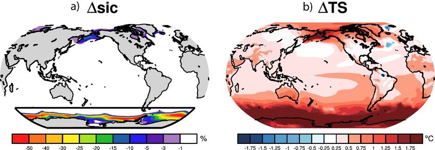
Let us start by examining the global impacts of ning of sea ice across the central Arctic (figure 3d).
Antarctic sea ice loss in the fully-coupled runs: the This Arctic response to Antarctic sea ice loss has
responses of sea ice and temperature—indicated by an important seasonal dependence. Since the Aleut-
the letter ∆ – are shown in figure 2 (for context, ian Low occurs primarily in boreal winter (Trenberth
we show the imposed annual mean Antarctic sea ice and Hurrell 1994, Bograd et al 2002, Gan et al 2017),
loss in the black box in panel 2a). First, we note the deepening of this low pressure circulation is found
that the response involves an overall surface warming to be strongest in that season (figure S3(b)). By con-
across the planet (figure 2b), with the largest increase trast, in boreal summer the North Pacific high extends
in the southern high-latitudes. The enhanced warm- further westward, limiting the extent of the Aleutian
ing in the tropical Pacific was documented in Eng- Low (Bograd et al 2002); the summertime mean sea
land et al (2020). Here, we focus on the pole-to-pole level pressure response involves high pressures across
impacts, notably the amplified surface warming in much of the northern high-latitudes with a swath of
3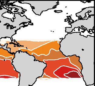
Environ. Res. Lett. 15 (2020) 104005                                                                                    M England et al

   Figure 1. Difference in prescribed SSTs ( ◦ C) between the two atmosphere-only runs, from the fully-coupled tropical response to
   Antarctic sea ice (England et al 2020).

   Figure 2. The annual mean response of (a) sea ice (in percentage) and (b) surface temperature (in ◦ C) to projected Antarctic sea
   ice loss. The imposed sea ice loss is shown in the black-bordered box at high Southern latitudes in (a).

low pressure further south across the North Pacific                   previous modeling (Yoo et al 2012, Kosaka and Xie
(figure S4(b)). Thus the warming response is largest                  2016, Svendsen et al 2018, Ding et al 2019, Screen and
in wintertime and weakest in summertime (compare                      Deser 2019, McCrystall et al 2020) and observational
figure S3(a) and figure S4(a)).                                       studies (Lee 2012, Ding et al 2014, Yoo et al 2014,
                                                                      Flournoy et al 2016, Hu et al 2016) which have identi-
                                                                      fied the tropical Pacific as a potential driver of Arctic
3.2. Connecting Antarctic sea ice loss to the Arctic                  warming.
Having shown that Antarctic sea ice loss can have                          We investigate this proposed mechanism by per-
important impacts on Arctic climate, we now ask:                      forming and analyzing two additional, atmosphere-
how does the signal reach all the way to the other                    only model simulations, to isolate the Arctic impacts
pole? We propose that the tropics play a key role                     of the tropical SST response to Antarctic sea ice loss.
in enabling these substantial pole-to-pole effects. As                These runs are detailed in section 2.3. In essence, one
documented in England et al (2020), Antarctic sea                     is a control simulation, the other is forced by the SSTs
ice loss in these model simulations causes enhanced                   in the control simulation plus the tropical SSTs anom-
surface warming and increased precipitation in the                    alies resulting from Antarctic sea ice loss in the fully-
Equatorial Pacific, as well as a warming of the trop-                 coupled model simulations (see figure 1). The differ-
ical upper troposphere (see figure 4a): ocean dynam-                  ence between these two runs illustrates the impact of
ics was shown to be key for connecting the loss of Ant-               such SST anomalies onto the Arctic, as communic-
arctic sea ice to the tropics. Now, we suggest that the               ated by the atmosphere alone.
tropical response signal is quickly propagated into the                    These prescribed-SST runs reveal five import-
Arctic by atmospheric teleconnections. Our suggested                  ant points. (i) As expected, the tropical upper
pathway is in line with the modeling study of Tomas                   tropospheric warming response to Antarctic sea ice
et al (2016), which showed that many of the impacts                   loss (figure 4a) is driven from below by the trop-
of Arctic sea ice loss on the northern mid- and high-                 ical SST anomalies (figure 4b). (ii) The tropical SST
latitudes are first mediated through the tropical SST                 anomalies cause amplified warming throughout the
response to sea ice loss. It is also consistent with the              lower troposphere in the Arctic (figure 4b), albeit

                                                       4
Environ. Res. Lett. 15 (2020) 104005 M England et al
Figure 3. The annual mean response of (a) 850hPa temperature ( ◦ C) , (b) sea level pressure (hPa), (c) sea ice concentration (in
percentage) and (d) sea ice thickness (m) to Antarctic sea ice loss in the fully-coupled simulations. The annual mean response of
(e) 850 hPa temperature ( ◦ C) and (f) sea level pressure (hPa) to prescribed tropical SSTs (see figure 1) in the atmosphere-only
configuration. Stippling indicates a statistically significant response at the 95% confidence level.
a)
b)
Figure 4. The latitude versus height cross section of the annual mean response of zonally averaged temperature ( ◦ C) to (a)
Antarctic sea ice loss in the fully-coupled configuration and to (b) prescribed tropical SSTs in an atmosphere-only configuration.
Stippling indicates a statistically significant response at 95% confidence.
somewhat smaller than in the fully-coupled Antarc- in response to tropical SST anomalies, as in the fully-
tic sea ice loss runs (figure 4a). This is clearly seen coupled runs, is related to a deepening of the Aleutian
in the warming response at 850 hPa (compare figure Low (compare figure 3b and figure 3f). This suggests
3a and figure 3e). (iii) The enhanced Arctic warming that the tropical SSTs anomalies, via a Rossby wave
5Environ. Res. Lett. 15 (2020) 104005 M England et al
Figure 5. The annual mean response of the 200 hPa eddy (deviation from the zonal mean) geopotential height (m) to (a)
Antarctic sea ice loss in the fully-coupled configuration and to (b) prescribed tropical SSTs in an atmosphere-only configuration.
Vectors indicate the annual mean response of wave activity flux (m2 s−2 ) (Takaya and Nakamura 2001) associated with the
200 hPa eddy geopotential height response. Vectors with a magnitude less than 1 m2 s−2 are omitted.
train, are also responsible for the deepened Aleu- this wave train is driven by Antarctic sea ice induced
tian Low—and accompanying Arctic warming—in changes in tropical SSTs because the same mechan-
response to Antarctic sea ice loss in the fully-coupled ism occurs in the atmosphere-only simulations in
runs. This is in agreement with the findings of Svend- response to prescribed tropical SSTs (figure 5(b)).
sen et al (2018), who identify the same mechanism as This wave train mechanism is largely consistent with
contributing to recent Arctic warming in the observed the one reported in the modelling and observational
record, as well as the modeling study of Screen and studies of Wettstein and Deser 2014, Tokinaga et al
Deser (2019). (iv) We are, of course, unable to dia- (2017), Svendsen et al (2018), Screen and Deser
gnose the response of Arctic sea ice cover to the trop- (2019), but opposite to the tropical-polar telecon-
ical SSTs anomalies because the surface conditions nections reported in Ding et al (2014), Baxter et al
are prescribed in the atmosphere-only runs; how- (2019), and Ding et al (2019). This discrepancy is
ever, both the near surface circulation response and likely explained by the differing spatial patterns of
the near surface warming in these runs are consist- anomalous SSTs imposed in these studies, especially
ent with a loss of Arctic sea ice in the Pacific sec- in the West Pacific. In addition, the fact that Baxter
tor. Finally, (v) the wintertime response to prescribed et al (2019) and Ding et al (2019) focus on the rela-
tropical SSTs anomalies well captures the response tionship between tropical SSTs and Arctic conditions
to Antarctic sea ice loss in the fully-coupled simu- in summer rather than the winter could play a role;
lations (compare the top and bottom rows in figure however it is also possible that climate models have
S3), whereas that response is much weaker, and less limitations in their representation of tropical-polar
similar, in the summertime (compare top and bottom linkages (Topal et al 2020).
rows in figure S4). Also, note that in that season the We conclude, therefore, that fast atmospheric
sea ice loss occurs most prominently over the cent- teleconnections from anomalous tropical SSTs offer a
ral Arctic (figure S4(c)), rather than over the Bering plausible pathway allowing the signal caused by Ant-
Sea (figure S3(c)). A different mechanism from the arctic sea ice loss to reach into the Arctic, with the
one examined here, in which the ocean and ice feed- amplitude of the Arctic response largest in the boreal
backs are likely involved and persist throughout the winter. This suggests that once the tropics begin to
year, may be needed to fully explain the summertime respond to Antarctic sea ice loss (England et al 2020),
response. which could take multiple decades owing to the long
We confirm that, in the coupled simulations, a timescale of the ocean response (Wang et al 2018),
Rossby wave train initiates in the tropical Pacific and the effects on the Arctic would then appear relatively
connects to the North Pacific, by showing the eddy quickly (on a timescale of years, rather than decades).
geopotential height response at 200 hPa and the asso- To be clear, the ocean plays a pivotal role in this pro-
ciated wave activity flux (figure 5(a)). It is clear that cess, because there is no Arctic response to Antarctic
6Environ. Res. Lett. 15 (2020) 104005 M England et al
sea ice loss in atmosphere-only model runs, as shown have proposed is likely a dominant one in facilitat-
in England et al (2018) (which use exactly the same ing the pole-to-pole response, especially in the boreal
model as the one employed here). winter.
Taken together, previous studies (e.g. Ding et al
4. Summary and Discussion 2014, Dong et al 2019, McCrystall et al 2020) sug-
gest that the Arctic response to tropical warming is
In this study, we have demonstrated the existence of a sensitive to the exact tropical forcing pattern and is
substantial Arctic impact from projected twenty-first likely model-dependent. This is an important caveat
century Antarctic sea ice loss. In our fully-coupled for our results, which are only based on one climate
climate model runs, in response to imposed Antarc- model. Consistent with our study, however, most
tic sea ice loss, the Aleutian Low deepens causing mechanisms that have been proposed to explain a
approximately 1 ◦ C warming in Arctic near-surface connection between the tropics and the Arctic have
air temperature ( 0.7 ◦ C at 850 hPa), with a larger been based on tropospheric Rossby waves initiat-
warming over the Bering Sea, East Siberia Sea, Chuk- ing in the tropical Pacific (Yuan et al 2018). In our
chi Sea, and Alaska regions than in the Atlantic sec- fully-coupled model simulations, we find warming
tor of the Arctic Ocean. The loss of Antarctic sea ice throughout the tropics, but the strongest warming is
also leads to an annual mean loss of 0.5 × 10⁶ km2 located in the Central and Eastern Equatorial Pacific
of sea ice extent in the Arctic, primarily in the Ber- (figure 1). However, results from Dong et al (2019),
ing Sea. With the aid of additional atmosphere-only in agreement with earlier studies (Yoo et al 2012,
model runs, we have shown that a fast atmospheric Ding et al 2019), suggest that the Arctic is respond-
response to the Antarctic-sea ice-loss-induced trop- ing primarily to the warming in the Western Equat-
ical SST anomalies is responsible for at least half of orial Pacific, the region of tropical ascent. Dong et al
this pole-to-pole signal. (2019) show that in abrupt 4 × CO2 experiments, des-
We acknowledge that the pole-to-pole effects doc- pite the Eastern Pacific warming more, it is the warm-
umented here are relatively small compared to the ing in the Western Pacific which is responsible for
internal variability of the climate system in the high- the temperature increase over the Arctic. Additional
latitudes. However, the polar cap warming and loss experiments with our atmosphere-only model could
of Arctic sea ice in our model are statistically signi- be carried out to test the relative importance of the
ficant at a 95% confidence level for every month of Eastern vs Western Tropical Pacific for Arctic climate
the year, not just in the annual mean. Furthermore, warming. However, such work is beyond the scope of
the sheer fact that as much as 10–15% of the end-of this short letter, whose primary goal is to highlight
the century Arctic warming projected under RCP8.5 the pole-to-pole impact of future Antarctic sea ice
could be induced from climate change at the oppos- loss.
ite pole offers a striking example of the huge geo-
graphical extent of the couplings at play among vari-
ous components in the Earth’s climate system. Acknowledgment
We also acknowledge that the magnitude of the
Arctic warming in our atmosphere-only runs with We appreciate the constructive feedback from two
prescribed tropical SST anomalies is, approximately, anonymous reviewers which have led to consider-
only half as large as the one in the fully-coupled runs able improvements in the manuscript. The work of
(compare figure 4a and 4e). It is important to appre- MRE is funded by grants OPP-1643445 and OPP-
ciate, however, that our aim was not to fully replic- 1744835 from the US National Science Foundation.
ate the exact Arctic response from the fully-coupled The work of LMP is funded, in part, by a grant from
simulations (which, in fact, may no be feasible with the US National Science Foundation to Columbia
an atmosphere-only model). Instead, our goal has University.
been to demonstrate a plausible pathway which could
explain the pole-to-pole connection. In fact, since Data Availability
prescribing SSTs and sea ice cover does not allow
them to freely evolve with the atmospheric condi- The data that support the findings of this study
tions, the Arctic warming response is likely underes- are available upon reasonable request from the
timated. For example, one would expect Arctic warm- authors.
ing to be amplified if sea ice cover is allowed to change,
via the sea ice albedo feedback. There may also be ORCID iDs
other pathways through which Antarctic sea ice loss
could influence the Arctic, the main candidates being M R England https://orcid.org/0000-0003-3882-
atmosphere-ocean coupling and ocean circulation 872X
changes which could alter the heat transport into the L M Polvani https://orcid.org/0000-0003-4775-
northern high-latitudes. However, the results presen- 8110
ted above suggest that tropics-to-pole mechanism we L Sun https://orcid.org/0000-0001-8578-9175
7Environ. Res. Lett. 15 (2020) 104005 M England et al
References Gan B et al 2017 On the response of the Aleutian Low to
greenhouse warming J. Clim. 30 3907–25
WMO 2018 Scientific Assessment of Ozone Depletion: 2018. Hu C et al 2016 Shifting El Nino inhibits summer Arctic warming
Global Ozone Research and Monitoring Project-Report No. and Arctic sea-ice melting over the Canada Basin Nat.
58 (Geneva: WMO) Commun. 7 11721
Ayres H and Screen J 2019 Multimodel analysis of the Kennel C and Yulaeva E 2020 Influence of Arctic sea-ice variability
atmospheric response to Antarctic sea ice loss at quadrupled on Pacific trade winds PNAS 117 2824–34
co2 Geophys. Res. Lett. 46 9861–9 Knutti R, Fluckiger J, Stocker T and Timmermann A 2004 Strong
Barbante Cet al and 2006 One-to-one coupling of glacial climate hemispheric coupling of glacial climate through freshwater
variability in Greenland and Antarctica Nature 444 195–8 discharge and ocean circulation Nature 430 851–6
Baxter I et al 2019 How Tropical Pacific surface cooling Kosaka Y and Xie S 2016 The tropical Pacific as a key pacemaker
contributed to accelerated sea ice melt from 2007 to 2012 as of the variable rates of global warming Nat. Geosci.
ice is thinned by anthropogenic forcing J. Clim. 32 8583–602 9 669–73
Blunier T et al 1998 Asynchrony of Antarctic and Greenland Lee S 2012 Testing of the Tropically Excited Arctic Warming
climate change during the last glacial period Nature Mechanism (TEAM) with traditional El Nino and La Nina J.
394 739–43 Clim. 25 4015–22
Blunier T and Brook E 2001 Timing of millennial-scale climate Liu W and Fedorov A 2018 Global impacts of Arctic sea ice loss
change in Antarctica and Greenland during the last glacial mediated by the Atlantic meridional overturning circulation
period Science 291 109–12 Geophys. Res. Lett. 46 944–52
Bograd S, Schwing F, Mendelssohn R and Green-Jessen P 2002 On Marino G, Rohling E, Rodriguez-Sanz L, Grant K, Heslop D,
the changing seasonality over the North Pacific Geophys. Res. Roberts A, Stanford J and Yu J 2015 Bipolar seesaw control
Lett. 29 9 on last interglacial sea level Nature 522 197–201
Broecker W 1998 Paleocean circulation during the last Marsh D, Mills M, Kinnison D and Lamarque J 2013 Climate
deglaciation: A bipolar seesaw? Paleoceanography 13 119–21 change from 1850 to 2005 simulated in CESM1(WACCM) J.
Chylek P, Folland C, Lesins G and Dubey M 2010 Twentieth Clim. 26 7372–91
century bipolar seesaw of the Arctic and Antarctic surface McCrystall M, Hosking J, White I and Maycock A 2020 The
air temperatures Geophys. Res. Lett. 37 L08703 impact of changes in tropical sea surface temperatures over
Cohen J et al 2020 Divergent consensuses on Arctic amplification 1979-2012 on Northern Hemisphere high latitude climate J.
influence on midlatitude severe winter weather Nat. Clim. Clim. 33 5103-5121
Change 10 20–9 Notz D et al 2020 Arctic sea ice in CMIP6 Geophys. Res. Lett. 47
Collins M et al 2006 Long-Term Climate Change: Projections, e2019GL086749
Commitments and Irreversibility chapter 12 (Cambridge, Parkinson C 2019 A 40-y record reveals gradual Antarctic sea ice
United Kingdom: Cambridge University Press) pp 1029–136 increases followed by decreases at rates exceeding the rates
Crowley T 1992 North Atlantic deep water cools the Southern seen in the Arctic PNAS 116 14414–23
Hemisphere Paleoceanography 7 489–97 Pedro J, Jochum M, Buizert C, He F, Barker S and Rasmussen S
De B and Wu Y 2019 Robustness of the stratospheric pathway in 2018 Beyond the bipolar seesaw: Toward a process
linking the Barents-Kara Sea sea ice variability to the understanding of interhemispheric coupling Quat. Sci. Rev.
mid-latitude circulation in CMIP5 models Clim. Dyn. 192 27–46
53 193–207 Pedro J, van Ommen T, Rasmussen S, Morgan V, Chappellaz J,
Deser C, Sun L, Tomas R and Screen J 2016 Does ocean coupling Moy A, Masson-Delmotte V and Delmotte M 2011 The last
matter for the northern extratropical response to projected deglaciation: timing the bipolar seesaw Climate of the Past
Arctic sea ice loss? Geophys. Res. Lett. 43 2149–57 7 671–83
Deser C, Tomas R, Alexander M and Lawrence D 2010 The Peings Y and Magnusdottir G 2014 Response of the wintertime
seasonal atmospheric response to projected Arctic sea ice Northern Hemisphere atmospheric circulation to current
loss in the late twenty-first century J. Clim. 23 333–51 and projected Arctic sea ice decline: A numerical study with
Deser C, Tomas R and Sun L 2015 The role of ocean-atmosphere CAM5 J. Clim. 27 244–64
coupling in the zonal-mean atmospheric response to Arctic Polvani L, Previdi M, England M, Chiodo G and Smith K 2020
sea ice loss J. Clim. 28 2168–86 Substantial twentieth-century Arctic warming caused be
Ding Q et al 2019 Fingerprints of internal drivers of Arctic ea ice ozone depleting substances Nat. Clim. Change 10 130–3
loss in observations and model simulations Nat. Geosci. Schneider D and Noone D 2012 Is a bipolar seesaw consistent
12 28–33 with observed antarctic climate variability and trends?
Ding Q, Wallace J, Battisti D, Steig E, Gallant A, Kim H and Geng Geophys. Res. Lett. 39 L06704
L 2014 Tropical forcing of the recent rapid Arctic warming Screen J and Deser C 2019 Pacific Ocean variability influences the
in northeastern Canada and Greenland Nature 509 209–12 time of emergence of a seasonally ice-free Arctic Ocean
Dong Y, Proistosescu C, Armour K and Battisti D 2019 Geophys. Res. Lett. 46 2222–2231
Attributing historical and future evolution of radiative Screen J, Deser C, Smith D, Zhang X, Blackport R, Kushner P,
feedbacks to regional warming patterns using a Green’s Oudar T, McCusker K and Sun L 2018 Consistency and
Function approach: The preeminence of the Western Pacific discrepancy in the atmospheric response to Arctic sea-ice
J. Clim. 32 5471–91 loss across climate models Nat. Geosci. 11 155–63
England M, Polvani L and Sun L 2018 Contrasting the Antarctic Screen J 2017 Far-flung effects of Arctic warming Nat. Geosci.
and Arctic atmospheric response to projected sea ice loss in 10 253–54
the late 21st Century J. Clim. 31 6353–70 Screen J, Simmonds I, Deser C and Tomas R 2013 The
England M, Polvani L, Sun L and Deser C 2020 Tropical climate atmospheric response to three decades of observed Arctic
responses to projected Arctic and Antarctic sea ice loss Nat. sea ice loss J. Clim. 26 1230–48
Geosci. 13 275–81 Screen J and Simmonds I 2010 The central role of diminishing sea
Fetterer F, Knowles K, Meier W N, Savoie M and Windnagel A K ice in recent Arctic temperature amplification Nature
2017 Sea Ice Index, Version 3 (Last accessed on April 31 464 1334–7
2020) https://nsidc.org/data/G02135/versions/3 Shepherd T 2016 Effects of a warming Arctic Science 353 989–90
Flournoy M, Feldstein S, Lee S and Clothiaux E 2016 Exploring Stocker T and Johnsen S 2003 A minimum thermodynamic
the tropically excited Arctic warming mechanism with model for the bipolar seesaw Paleoceanography 18
station data: Links between tropical convection and Stocker T 1998 The seesaw effect Science 282 61–62
Arctic downward infrared radiation J. Atmos. Sci. Stuecker M et al 2018 Polar amplification dominated by local
73 1143–58 forcing and feedbacks Nat. Clim. Change 8 1076–81
8Environ. Res. Lett. 15 (2020) 104005 M England et al
Sun L, Deser C, Tomas R and Alexander M 2020 Global coupled Trenberth K and Hurrell J 1994 Decadal
climate response to polar sea ice loss: Evaluating the atmosphere-ocean variations in the Pacific Clim. Dyn.
effectiveness of different ice-constraining approaches 9 303–19
Geophys. Res. Lett. 47 e2019GL085788 Wang K, Deser C, Sun L and Tomas R 2018 Fast response of the
Sun L, Deser C and Tomas R 2015 Mechanisms of stratospheric tropics to an abrupt loss of Arctic sea ice via ocean dynamics
and tropospheric circulation response to projected Arctic Geophys. Res. Lett. 45 4264–4272
sea ice loss J. Clim. 28 7824–45 Wang Z, Zhang X, Guan Z, Sun B, Yang X and Liu C 2015 An
Svendsen L, Keenlyside N, Bethke I, Gao Y and Omrani N 2018 atmospheric origin of the multi-decadal bipolar seesaw Sci.
Pacific contribution to the early twentieth-century warming Rep. 5 8909
in the Arctic Nat. Clim. Change 8 793–7 Wettstein J and Deser C 2014 Internal variability in projections of
Takaya K and Nakamura H 2001 A formulation of a twenty-first-century Arctic sea ice loss: Role of the
phase-independent wave activity flux for stationary and large-scale atmospheric circulation J. Clim.
migratory quasigeostrophc eddies on a zonally varying basic 27 527–50
flow J. Atmos. Sci. 58 608–27 Yoo C, Feldstein S and Lee S 2014 The prominence of a tropical
Tokinaga H, Xie S and Mukougawa H 2017 Early 20th-century convective signal in the wintertime Arctic temperature
Arctic warming intensified by Pacific and Atlantic Atmos Sci Lett 15 7–12
multidecadal variability PNAS 114 6227–32 Yoo C, Lee S and Feldstein S 2012 Arctic response to an MJO-like
Tomas R, Deser C and Sun L 2016 The role of ocean heat tropical heating in an idealised GCM J. Atmos. Sci.
transport in the global climate response to projected Arctic 69 2379–93
sea ice loss J. Clim. 29 6841–59 Yuan X, Kaplan M and Cane M 2018 The interconnected global
Topal D, Ding Q, Mitchell J, an M, Herein I B, Haszpra T, Luo R climate system - a review of tropical-polar teleconnections J.
and Li Q 2020 An internal atmospheric process determining Clim. 31 5765–92
summertime Arctic sea ice melting in the next three decades: Zhang P, Wu Y, Simpson I, Smith K, Zhang X, De B and
Lessons learned from five large ensembles and multiple Callaghan P 2018 A stratospheric pathway linking a colder
CMIP5 climate simulations J. Clim. 33 7431–7454 Siberia to Barents-Kara Sea sea ice loss Sci. Adv. 4 eeat6025
9You can also read