Extracting Analyzing and Visualizing Triangle K-Core Motifs within Networks
←
→
Page content transcription
If your browser does not render page correctly, please read the page content below
Extracting Analyzing and Visualizing Triangle
              K-Core Motifs within Networks
                                          Yang Zhang #1 , Srinivasan Parthasarathy #2
                         #
                             Department of Computer Science and Engineering, The Ohio State University
                                            2015 Neil Ave, Columbus, OH 43202, USA
                                                         1
                                                           zhang.863@osu.edu
                                                   2
                                                       srini@cse.ohio-state.edu

   Abstract—Cliques are topological structures that usually pro-       in its own right, since the exact clique discovery problem is
vide important information for understanding the structure of          not only NP-Hard but is also very hard to approximate [1].
a graph or network. However, detecting and extracting cliques             In this article we attack a small region of this problem space.
efficiently is known to be very hard. In this paper, we define and
introduce the notion of a Triangle K-Core, a simpler topological       Specifically, we develop a scalable visual-analytic framework,
structure and one that is more tractable and can moreover be           for probing and uncovering dense substructures within net-
used as a proxy for extracting clique-like structure from large        works. Central to our approach is the novel notion of a
graphs. Based on this definition we first develop a localized          Triangle K-Core motif. We develop a simple algorithm for
algorithm for extracting Triangle K-Cores from large graphs.           computing Triangle K-Cores from graphs. We then discuss
Subsequently we extend the simple algorithm to accommodate
dynamic graphs (where edges can be dynamically added and               a mechanism to plot such Triangle K-Cores – essentially
deleted). Finally, we extend the basic definition to support various   realizing a density plot in a manner analogous to a CSV
template pattern cliques with applications to network visualization    plot[2]. This plot follows an Optics[3]-style enumeration of
and event detection on graphs and networks. Our empirical              vertices in the network. The proposed algorithm is provably
results reveal the efficiency and efficacy of the proposed methods     efficient on several real world scale-free (sparse) social and
on many real world datasets.
                                                                       biological networks. In fact as our experimental results show,
                      I. I NTRODUCTION                                 we produce plots that are very similar to CSV at a fraction
   Many real world problems can be modeled as complex                  of the cost. Moreover, our empirical results suggest that
entity-relationship networks where nodes represent entities            Triangle K-Cores motifs, can be used as preprocessing step
of interest and edges mimic the relationships among them.              for detecting exact cliques as demonstrated elsewhere[2].
Fueled by technological advances and inspired by empirical                Subsequently we extend the above static algorithm to handle
analysis, the number of such problems and the diversity of             dynamic graphs. A key challenge addressed here is that
domains from which they arise – physics, sociology, technol-           of cognitive correspondence – the same community in two
ogy, biology, chemistry, metabolism and nutrition – is growing         different density plots must be clearly identified as long as
steadily. The study of such networks can help us understand            the local relationship structure has not changed significantly.
the structure and function of such systems, potentially allowing       We develop a suitable incremental algorithm, with cognitive
one to predict interesting aspects of their behavior.                  correspondence (by relying on an adaptation of dual-view
   Of particular interest in many of these applications, is            plots), which we show to be significantly faster than the naive
the ability to probe, uncover, and understand the evolution            approach which recomputes Triangle K-Cores from scratch.
of dense structures (communities or cliques) within such                  An additional feature of our algorithms is the ability for the
networks. The challenges are daunting and manifold. First,             domain expert to dynamically specify, explore and probe the
the topological characteristics of the data (scale-free nature,        network for various user-defined template patterns of interest
presence of hub nodes) as well as the size of the data poses           defined upon the Triangle K-Core. Such template patterns can
an inherent challenge. Second, often such data is dynamic in           be extremely informative. We design and adapt our density
nature which in turn requires identifying the portions of the          plot framework (here density is defined by the density of the
network that have changed, characterizing the type of change,          template pattern of interest) based on this notion and discuss
and developing models for evolving community structures.               several applications of this work on real world datasets. To sum
Third, fundamental to most data analysis is visual confirmation        up, the main contribution of our work is to introduce a new
– from Galileo seeing the moons of Jupiter to Gerd Binnig and          motif for estimating clique like structure in graphs (Triangle
Heinrich Rohrer seeing atoms on a surface. Visualizing such            K-Core). Specifically in this article we demonstrate its:
complex networks and honing in on important and possibly                  1) Utility: We demonstrate its use for visualization (in a
evolving topological characteristics is difficult, given the size             manner similar to a CSV plot), probing, exploring and
and complexity of such systems, but nonetheless important.                    highlighting interesting patterns in both static as well
Finally, the scale and complexity of such networked data                      as dynamic graphs. We compare its utility with respect
dictate the need for efficient solutions – a grand challenge                  to recent state of the art alternative (e.g. CSV[2] and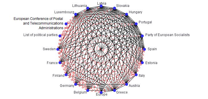
DN-Graph[4] motifs.                                            graph visualization system which uses clustering to construct
  2) Efficiency: We present a localized algorithm for extract-      a hierarchy of large scale graphs.
     ing such motifs and demonstrate its efficiency by several
                                                                                             III. P RELIMINARIES
     factors over competing strategies such as DN-Graph[4]
     and CSV[2]. Additionally, we present an incremental               Given a graph G = {V ,E}, V is the set of distinct vertices
     variant that can be extended to handle dynamic graphs          {v1 , ..., v|V | }, and E is the set of edges {e1 , ..., e|E| }. A graph
     with much lower cost than the iterative method[4] and          G′ = {V ′ ,E ′ } is a subgraph of G if V ′ ⊆ V , E ′ ⊆ E.
     global method[2] used by extant approaches.                       The Triangle K-Core subgraph proposed in this paper is
  3) Flexibility: An important feature of the Triangle K-           derived from K-Core subgraph, and we explain and compare
     Core motif is its inherent simplicity which lends itself       them as follows.
     to flexible probing of user-defined pattern cliques of            Definition 1: A K-Core is a subgraph G′ of G that each
     interest within both static and dynamic graphs.                vertex of G′ participates in at least k edges within the subgraph
                                                                    G′ . The K-Core number of such a subgraph is k.
                      II. R ELATED W ORK                               Definition 2: The maximum K-Core associated with a
   In the context of graph clustering, several methods have         vertex v is defined by the subgraph Gv containing v whose
often found favor. For example, spectral methods[5], stochastic     K-Core number is the maximum from among all subgraphs
flow methods[6], multi-level methods[7], [8] have all been          containing v. The K-Core number of Gv is the maximum
used for discovering dense subgraphs of interest. While several     K-Core number of v.
of these algorithms scale well to large datasets they do not           Batagelj et al [21] propose an efficient method to compute
precisely target the problem of detecting clique-like structures.   every vertex’s maximum K-Core number with O(|E|) time
   In spite of the fact that CLIQUE problem is NP-Hard[9],          complexity.
and approximating the size of the largest clique in a graph            Based on definition of K-Core, we are now in a position to
is almost NP-complete[1], mining cliques for a graph has            define the notion of a Triangle K-Core:
received much attention recently. The CLAN method [10] for             Definition 3: A Triangle K-Core is a subgraph G′ of G
example, aims to mine exact cliques in large graph datasets,        that each edge of G′ is contained within at least k triangles
CLAN uses the canonical form to represent a clique, and             in the subgraph. Analogously, the Triangle K-Core number
the clique detection task becomes mining strings representing       of this Triangle K-Core is refered to as k.
cliques. Some other methods[11], [12] have been proposed               Definition 4: The maximum Triangle K-Core associated
to detect quasi-clique, which is a clique with some edges           with an edge e is the subgraph Ge containing e that has the
missing. Wang et al.[2] propose CSV to visualize approximate        maximum Triangle K-Core number. Analogously, the Triangle
cliques. CSV uses a notion of local density, co-clique size,        K-Core number of Ge is the maximum Triangle K-Core
and plots all vertices based on co-clique sizes. The plot is a      number of edge e. We use κ(e) to denote the maximum
OPTICS [3] style plot, and visualizes the distribution of all       Triangle K-Core number of edge e.
the potential cliques. However, calculating co-clique size in          The main advantage of a Triangle K-Core over a K-Core is
CSV is still fairly expensive and makes CSV costly on large         that it offers a natural approximation of clique, we illustrate
scale graphs. Other clique-like dense subgraph patterns, such       this in the Figure 1.
as DN-graph[4], are also expensive to compute.
   Many methods have been proposed to analyze dynamically
changing graphs. Leskovec et al.[13] study the topological
properties of some evolving real-world graphs, and propose
“forest fire” spreading process including these properties.
Backstrom et al.[14] study the relation between the evolution                 (a) K-Core Number = 2      (b) Triangle K-Core Number = 2
of communities and the structure of the underlying social
                                                                                      Fig. 1.   K-Core vs. Triangle K-Core
networks. Asur et al.[15] define several events based on graph
clusters evolution, and analyze group behavior through these           Figure 1(a) is a 5-vertex K-Core with K-Core number 2
events. Sun et al.[16] present a non-user-defined parameters        constructed by minimal number of edges, Figure 1(b) is a
approach to cluster evolving graphs based on Minimum De-            5-vertex Triangle K-Core with Triangle K-Core number 2
scription Length principle. Lin et al.[17] propose FacetNet         constructed by minimal number of edges, and we can easily
framework to detect community structure both by the network         see that the Triangle K-Core is much closer to a 5-vertex clique
data and the historic community evolution patterns.                 than the K-Core. In fact, Triangle K-Core is a relaxation of
   Graph visualization is often helpful for providing important     clique, a n-vertex clique is equivalent to a n-vertex Triangle
insights of graph datasets. Namata et al.[18] develop a dual-       K-Core with Triangle K-Core Number n-2.
view approach to provide multiple views of a network simul-            The Triangle K-Core motif is based on triangles of each
taneously. Yang et al.[19] propose a Visual-Analytic Toolkit to     edge rather than each node, the intuition is, for example, an
help analyze behavioral properties of nodes and communities,        edge participating in 4 triangles implies a subgraph of 6 nodes
such as stability and influence. Abello et al.[20] propose a        and 9 edges (in the worst case). A node participating in 4
triangles could involve 9 nodes and 12 edges(a hub-pattern             K-Core, so in step 5 the algorithm (AddToCore), updates its
in the worst case). The former is closer to a 6-node clique            bookkeeping to reflect the fact that each triangle t is possibly
(density: 9/15=60%) than the latter to a 9-node clique(density:        in e’s maximum Triangle K-Core. Finally, κ̃(e) contains the
12/36=33%). Note that a Triangle K-Core makes an even                  upper bound of e’s maximum Triangle K-Core number κ(e).
stronger assertion on density, since it requires every edge is            In step 7 we place all the edges in a list sorted by increasing
contained within at least k triangles.                                 order of κ̃ value. Bucket sort can be used as an optimization
   For edge et and a triangle T containing et , we have the            step here with time complexity O(|E|). In steps 8-18, we pro-
following property for T:                                              cess each edge ei and determine its exact maximum Triangle
   Theorem 1: If triangle T is in et ’s maximum Triangle K-            K-Core number κ(ei ) since thus far we only had an upper
Core, and contains three edges, et , e1 and e2 , then κ(ei ) ≥         bound. In step 10, we determine that κ(ei ) is exactly κ̃(ei ),
κ(et ) (i = 1,2).                                                      the correctness is proved later. Then we update ei ’s neighbor
      Proof: Since edge ei is in triangle T, and T is in et ’s         edges’ κ̃ value in steps 11-17. If an unprocessed triangle T on
maximum Triangle K-Core, denoted as Get , we have subgraph             ei contains edge et that κ̃(et ) is greater than κ̃(ei ) (step 13),
Get contains ei . According to Definition 4, ei ’s maximum             we delete T from the upperbound of et ’s maximum Triangle
Triangle K-Core should have Triangle K-Core number no less             K-Core. DelFromCore updates its bookkeeping to indicate that
than Get ’s Triangle K-Core number, that is κ(ei ) ≥ κ(et ).           T is not in the upperbound of et ’s maximum Triangle K-Core.
                                                                       In step 16, based on bucket sort the update could be optimized
               IV. T RIANGLE K-C ORE A LGORITHM                        with complexity O(1).
A. Detecting Maximum Triangle K-Core                                      In fact, steps 5 and 14 are not necessary here, but it will be
   In Algorithm 1, input is Graph G, output is the maximum             useful for dynamic update algorithms. The time complexity for
Triangle K-Core number and optionally the maximum Triangle             steps 1-7 is O(Σ(d2i )), di is the degree for node i, i=1,2...|V |.
K-Core associated with each edge. In each iteration, this              The time complexity for Steps 8-18 is O(|T ri| + |E|), where
algorithm processes a particular edge ei and determines its            |T ri| is the total number of triangles in the graph.
maximum Triangle K-Core number.

Algorithm 1 Detect each edge’s maximum Triangle K-Core
 1: for each edge e in the graph do
 2:    set e to be unprocessed;
 3:    find all the triangles on e, set them to be unprocessed;                        (a) Example of Algo. 1   (b) Example of Algo. 2
 4:    for each triangle t on edge e do
 5:       AddToCore(t, e);                                                   Fig. 2.   Examples for Illustrating Triangle K-Core Algorithms
 6:       κ̃(e) + +;
 7: Place all the edges in list Edges, sort them in increasing order      Example: Figure 2(a) is an example to illustrate Algo-
      of κ̃ value;
 8:   for i = 0 to |E|−1 do                                            rithm 1. We find the triangles on each edge, and sort edges
 9:      ei = Edges[i];                                                in increasing order of κ̃ value, {AB(1), AC(1), BD(2), BE(2),
10:      κ(ei ) = κ̃(ei );                                             CD(2), CE(2), DE(2), BC(3)}, where the number in parenthe-
11:      for each unprocessed triangle T on ei do                      sis indicates the κ̃ value of the edge. We process AB first, and
12:         for each edge et other than ei in T do                     get κ(AB)=1. For unprocessed △ABC on AB, κ̃(BC)=3 is
13:            if κ̃(et ) > κ̃(ei ) then
14:                DelFromCore(T, et );                                greater than κ̃(AB)=1, so κ̃(BC) decrease 1 to be 2 (step 15),
15:                κ̃(et ) − −;                                        and △ABC becomes processed. Then we process edge AC,
16:                update et ’s position in the sorted list Edges;     and have κ(AC)=1, there is no unprocessed triangle on AC,
17:         set triangle T to be processed;                            so no update is needed. Next we process edge BD, and get
18:      set ei to be processed;                                       κ(BD)=2, △BDC and △BDE on BD are unprocessed, but
                                                                       no edge of the two triangles has greater κ̃ value than κ̃(BD),
   Before describing the Algorithm 1 we define the notions             so no update. In the same way we find all left edges having
of processing an edge and a triangle. If an edge’s maximum             κ value equals 2.
Triangle K-Core number has been determined, it is considered              Proof of Correctness of Algorithm 1: We show the
to be processed. A triangle T is processed if any one of its           following invariances of Algorithm 1: at the end of each
edges is processed.                                                    iteration i, (1)for the edge et whose κ̃(et ) value updated, κ̃(et )
   In step 2, each edge is set to unprocessed. In step 3, each         is still the upperbound of κ(et ); (2) for the edge ei processed
triangle on edge e is constructed by e’s two vertices and one          in current iteration, κ̃(ei ) is equal to κ(ei ).
common neighbor of them. One triangle could be constructed                We firstly prove the invariance (1) of Algorithm 1. In steps
three times by its three edges, but we only store one instance         11-12, for an unprocessed triangle T on edge ei , all T’s edges
of each triangle, by giving a unique id to each edge and only          are unprocessed, so T is still in the upperbound of maximum
creating a triangle instance on its edge with smallest id. Note        Triangle K-Cores of all its edges(including edge ei and et ). If
that all triangles on edge e could be in e’s maximum Triangle          κ̃(et ) > κ̃(ei ) (step 13), we have: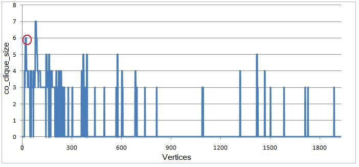
Claim 1: κ̃(et ) > κ(et )                                          edges whose maximum Triangle K-Cores might change, and
      Proof: We prove by contradiction. Assume κ̃(et ) = κ(et ),      store them in PotentialList. We use Rule 0 to help find the
then all the triangles in the current upper bound of et ’s            edges whose maximum Triangle K-Cores might change. Rule
maximum Triangle K-Core are exactly in et ’s maximum                  0 is derived from Theorem 1, the proof is omitted for brevity.
Triangle K-Core, so T is in et ’s maximum Triangle K-Core.               • Rule 0: when triangle t is added/deleted to graph G,
However, in triangle T, κ(et ) = κ̃(et ) > κ̃(ei ) >= κ(ei ),              assume µ is smallest κ value of t’s three edges, then
which violates Theorem 1, so the assumption is incorrect. We               only the edges in G whose κ value equals µ might have
have κ̃(et ) > κ(et ).                                                     their maximum Triangle K-Cores changed.
According to the proof of Claim 1, after decreasing κ̃(et ) by        Then we process each edge e in PotentialList to update its
1 (step 15), κ̃(et ) still remains as the upper bound of κ(et ).      κ(e). All the triangles associated with edge e should obey
So invariance (1) is held.                                            Theorem 1, so we process them based on Theorem 1 (steps
   Now we prove invariance (2). In iteration i, assume κ̃(ei ) =      6-7). If κ(e) finally changes, we put e in ChangingList,
k, we use the edges whose current κ̃ ≥ k to construct a               which stores edges whose κ(e) has been changed, and put
subgraph Gk (including ei ), and have the following claim:            e’s neighbor edges whose maximum Triangle K-Cores might
   Claim 2: The subgraph Gk is a Triangle K-Core with                 change to PotentialList(step 8). We use Rule 0 to help select
Triangle K-Core number k.                                             the edges to be put in PotentialList. After processing all edges
      Proof: For any edge e in Gk , κ̃(e) ≥ k, so the upper           in PotentialList, we could determine edges’ maximum Triangle
bound of e’s maximum Triangle K-Core now contains at least            K-Core numbers in ChangingList(step 9).
k triangles. Assume triangle T is one of them, considering T’s           Please note that if an added triangle is not updated, or a
two other edges e1 and e2, if e1 is not in subgraph Gk , then         deleted triangle is updated, we do not involve them in the
κ̃(e1) < k. We could see that Algorithm 1 processes edges             Algorithm 2. A brief illustration of Algorithm 2 is as follows.
in increasing order of κ̃, so e1 should already be processed.
When processing e1, κ̃(e1) < κ̃(e) (step 13) is true, so triangle     Algorithm 2 Update maximum Triangle K-Cores
T should be deleted from the upper bound of e’s maximum                1: for each added/deleted triangle T do
Triangle K-Core (step 14), which is a contradiction to the             2:    Set T to be updated;
assumption that triangle T is in upper bound of e’s maximum            3:    Put T’s edges whose maximum Triangle K-Cores might
                                                                            change to PotentialList;
Triangle K-Core. So e1 is in subgraph Gk , and so is e2.               4:   Add/delete T from the maximum Triangle K-Cores of edges
Because edges e, e1 and e2 are all in subgraph Gk , triangle                in PotentialList, update those edges’ κ value;
T is in Gk . So all the triangles now in upper bound of e’s            5:   for each edge e in PotentialList do
maximum Triangle K-Core are in subgraph Gk , which means               6:      Find e’s “illegal” triangles that violate Theorem 1;
any e in Gk is contained in at least k triangles in Gk , so Gk         7:      Process e’s “illegal” triangles to obey Theorem 1, mean-
                                                                               while update κ(e);
is a Triangle K-Core with Triangle K-Core number k.                    8:      If κ(e) changes, put e in ChangingList, put e’s neighbor
In Claim 2, we have a subgraph Gk containing ei with Triangle                  edges whose maximum Triangle K-Cores might change to
K-Core number equals κ̃(ei ), so κ̃(ei ) is exactly κ(ei ), invari-            PotentialList;
ance (2) is held, and Gk is obviously the maximum Triangle             9:   update κ(e) of each edge e in ChangingList;
K-Core of ei .
   In step 3 we could store all triangles in main memory, then           Example: In Figure 2(b), the original graph is comprised
reuse them in step 11. However for a large graph, storing             with solid edges, and edge AC is added. The original κ value
all triangles in main memory might be impossible. In such             for each edge is {AB(0), BC(0), AE(1), AF(1), EF(1), CD(1),
a case, we do not store triangles in step 3, and compute              CE(1), DE(1)}. The initial value for κ(AC) is 0. After adding
each edge’s triangles again in step 11, then we test whether a        edge AC, two triangles are added, △ABC and △AEC.
triangle is unprocessed by testing whether its three edges are           Firstly, we process newly added △ABC, now all its three
all unprocessed.                                                      edges are {AB(0), BC(0), AC(0)}, so we put all three edges
                                                                      in PotentialList (Rule 0), and add △ABC to their maximum
B. Updating Maximum Triangle K-Core                                   Triangle K-Cores (step 4), their κ value increases to be 1.
   So far we have worked on static graphs. In scenarios when          Then we process each edge in PotentialList, assume AC is the
edges are added and removed from a graph over time however,           first edge. In step 6 we find △ABC on edge AC is “legal”,
rather than recomputing the Triangle K-Cores from scratch             and △AEC is not taken into consideration because it is not
after each change, we can use Algorithm 2 to efficiently update       updated. In step 8, because κ(AC) changes to be 1, we put
edges’ maximum Triangle K-Cores. The detailed pseudo code             edge AC’s neighbor edges AB, BC in PotentialList(they are
of Algorithm 2 is in Appendix (Section IX-A).                         already in). In the following iterations we process left edges in
   Adding/deleting one edge might add/delete multiple trian-          PotentialList (AB and BC) similarly, and update κ(AB) and
gles simultaneously, in Algorithm 2 we process added/deleted          κ(BC) to be 1.
triangles one by one (step 1). Initially all added/deleted               Then, we process newly added △AEC, now its three edges
triangles are not updated, and when processing one triangle           are {AE(1), EC(1), AC(1)}, so we put all of them in Poten-
T we set it to be updated (step 2). In step 3, we identify T’s        tialList, and add △AEC to their maximum Triangle K-Cores,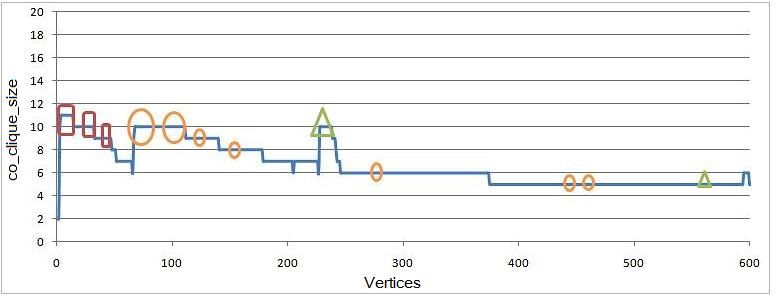
their κ value increases to be 2. Let’s process edge AC first, we   Algorithm 3 Dual View Plots
find △ABC on edge AC is “illegal”, because △ABC is in               1: Execute Algorithm 1 to compute κ(e) for each edge e in Ga ;
AC’s maximum Triangle K-Core while κ(AC) = 2 is greater             2: For each edge e in Ga , e.co clique size = κ(e) + 2;
                                                                    3: Plot clique distribution of Ga (plot(a));
than κ(BC) = 1 and κ(AB) = 1, which violates Theorem 1.             4: After Ga evolves to be Gb by adding new edges, execute
So in step 7 we delete △ABC from AC’s maximum Triangle                 Algorithm 2 to update κ(e) for each edge e in Gb ;
K-Core and decrease κ(AC) to be 1. Similarly edges AE and           5: For each edge e in Gb , if e is newly added edge,
EC in PotentialList both are processed to decrease κ(AE) and           e.co clique size = κ(e) + 2, otherwise e.co clique size = 0;
κ(EC) to be 1.                                                      6: Plot clique distribution of Gb (plot(b)) based on co clique size
                                                                       calculated in step 5;
   The proof of correctness of Algorithm 2 and Rule 0 is in our     7: In plot(b) select one Clique C of interest, locate the corresponding
technical report[22]. If we do not store triangles in Algorithm        vertices of C in plot(a), and analyze how C is formed;
1, then in Algorithm 2 we need to recompute triangles from
edges, we explain this in Appendix (Section IX-A).
                                                                   merging two cliques in a previous snapshot, or by augmenting
                        V. E XTENSIONS                             a clique in previous snapshot. Such cliques can allow a
Visualizing Clique-like Structures: We now describe how            user to probe an evolving network to discover interesting or
Triangle K-Cores can be used for detecting and visualizing         anomalous behavior[23]. The end-goal of our method is to
interesting clique-like structures within networks. Before de-     allow the user the flexibility to specify what patterns are of
scribing our technique we briefly review the CSV method [2]        interest to her/him in the context of the domain.
to visualize all potential cliques in graph.                          Several examples of template pattern cliques in evolving
   CSV plot: CSV first estimates co clique size for each edge,     graphs are illustrated in Figure 3. The previous snapshot of the
which is the size of the maximum clique that each edge             graph is denoted as Gold , the current snapshot is denoted as
participants in. Then subsequently CSV plots vertices along        Gnew . In Figure 3 black vertices/edges are old vertices/edges,
X-axis in a certain order, and the Y-axis value for each vertex    i.e., vertices/edges in Gold , red vertices/dashed-lines are
is one of its neighbor edges’ co clique size value. The final      newly added vertices/edges in Gnew . The template pattern
plot is the clique distribution of the graph, and the flat peaks   cliques defined below are all in Gnew .
in the plot indicate potential cliques.                            1. An Emerging Clique is formed by connecting old vertices
   However, estimating co clique size for each edge takes up       with newly added edges. In Figure 3(a) ABCDE is an
most of the time cost in CSV. Instead we propose to use each       Emerging Clique.
edge’s maximum Triangle K-Core as a proxy to approximate           2. A Bridge Clique is formed by connecting two disconnected
the maximum clique it participates in. Since the maximum           cliques in Gold with newly added edges. In Figure 3(b)
clique among a subgraph with Triangle K-Core Number κ              ABCDE is a Bridge Clique.
is a (κ + 2)-vertex clique, we estimate e.co clique size as        3. An Expanding Clique is formed by augmenting a clique
κ(e) + 2 for each edge e, and then plot the clique distribution    in Gold with newly added vertices and edges. In Figure 3(c)
using the same method as that of CSV. As we demonstrate            ABCDEF is an Expanding Clique.
in experiments our method produces plots that are inherently
similar or identical to that of CSV at a fraction of the cost.
Dual View Plots: In a graph G that evolves over time, when
edges are added to it, some clique structures in G might
change. We propose Dual View Plots to analyze how clique
structures in G change over time.
   The idea is: for one snapshot Ga of graph G, we plot all
its cliques in plot(a). After Ga evolves to be snapshot Gb by            (a) Emerging Clique:     (b) Bridge          Clique:    (c)      Expanding
                                                                         ABCDE                    ABCDE                          Clique: ABCDEF
adding new edges, in plot(b) we plot the cliques of Gb that
contain new edges, these cliques should not exist in Ga , and
they are usually formed by merging/expanding cliques in Ga .
By comparing plot(a) and plot(b), we can visually analyze how      (d) Characteristic triangle   (e) Characteristic triangle    (f) Characteristic triangle
cliques in plot(b) are formed from cliques in plot(a). We use      of Emerging Clique            of Bridge Clique               of Expanding Clique
the the same plot method as CSV to plot clique distribution.        Fig. 3.    Several template pattern cliques and their characteristic triangles
The detailed steps are presented in Algorithm 3. We illustrate
the benefits of Dual View Plots in the Section VII Experiments.       We propose Algorithm 4 to detect and extract the template
                                                                   pattern cliques of interest. We first define the notion of a char-
Detecting Template Pattern Cliques: In this section we             acteristic triangle within an evolving network. The vertices
describe a method which allows users to detect cliques of          and edges of a characteristic triangle are labeled as new(red)
patterns of their interest, which we call template pattern         or old(black), as defined above. Two labeled characteristic
cliques. For example, in one snapshot of a graph that evolves      triangles are of the same type if they are isomorphic. A
over time, template pattern cliques might be cliques formed by     template pattern clique is identified uniquely with a single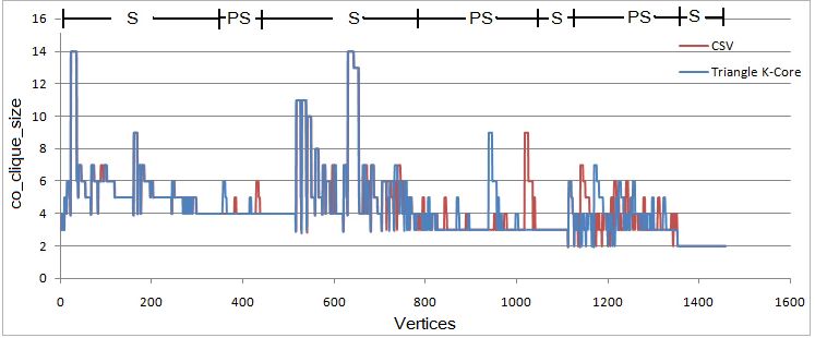
characteristic triangle type (see Figure 3 for examples), and        Algorithm 4 Detecting template pattern cliques in Graph G
every vertex (this does not hold for every edge as we shall           1: Define and detect the characteristic triangles of the template
clarify shortly) within a template pattern clique of interest will      pattern cliques;
                                                                      2: for each characteristic triangle Tc do
participate in at least one characteristic triangle of the given      3:    Mark Tc ’s edges and vertices as selected;
type (again see Figure 3). Thus the vertices of all template          4: Define and detect the possible triangles formed by selected
pattern cliques are a subset of the vertices of all characteristic      vertices;
triangles of the given type.                                          5: for each possible triangle Tp do
   We note that besides characteristic triangles, other types of      6:    Mark Tp ’s edges as selected;
                                                                      7: Extract the subgraph Gsel built by selected vertices and selected
triangles can also occur within template pattern cliques – we           edges;
call these possible triangles, and they account for the edges         8: Execute Algorithm 1 on Gsel to calculate each selected edge’s
that do not occur within characteristic triangles (e.g., edge           κ value;
AB in Figure 3(c)). Obviously the vertices of these possible          9: for each edge e in G do
triangles are among the vertices of characteristic triangles.        10:    if e is a selected edge then
                                                                     11:       e.co clique size = κ(e)+2;
   Thus identifying all characteristic triangles and possible        12:    else
triangles of the given type within the evolving network will         13:       e.co clique size = 0;
cover all the vertices and edges in the template pattern             14: Use the same plot method as CSV to plot clique distribution of
cliques, and plotting their density plot (using Triangle K-Core)        graph G;
will ensure the complete detection and extraction of relevant
template pattern cliques. Note that such a density plot will
now highlight the regions of the network where the densest           have different labels. In Section VII Experiments we will
template clique patterns of interest are found as opposed            illustrate detecting template pattern cliques on both static and
to simply the densest clique structures. In the following we         dynamic graphs.
specify the characteristic triangles and possible triangles of
the three template pattern cliques introduced before.                               VI. R ELATIONSHIP TO DN-G RAPH
   Detect Emerging Cliques: the characteristic triangle of an
Emerging Clique has 3 new edges and 3 old vertices, as                  Before we discuss the empirical evaluation we would like to
illustrated in Figure 3(d), and no possible triangles are in         highlight an interesting connection between our approach and
Emerging Cliques.                                                    the recent approach proposed by Wang et al.[4]. It is interest-
   Detect Bridge Cliques: the characteristic triangle of Bridge      ing to note that this connection was initially observed during
Clique has 3 old vertices, 2 new edges, and 1 old edge, as           our empirical evaluation, where we found both DN-Graph and
illustrated in Figure 3(e). We find that in Bridge Clique there      our method converge to identical values of co clique size
is one type of possible triangle, which is comprised of 3 old        (density). We are now in a position to also provide a theoretical
edges and 3 old vertices, such as △BCD in the Figure 3(b).           justification for this connection.
   Detect Expanding Cliques: the characteristic triangle of             DN-Graph G’(V’, E’, λ) is a subgraph pattern proposed by
Expanding Clique contains 1 new vertex, 2 old vertices, 2            Wang et al.[4], it satisfies two requirements
new edges, 1 old edge, as Figure 3(f) shows. There are two           (1) every connected pair of vertices in G’ has at least λ
types of possible triangles in Expanding Clique. One type is         common neighbors; (2) for a vertex v not in G’, adding v
made of all new edges, such as △ABC in the Figure 3(c),              to G’ will decrease the λ value of G’, for vertex v’ in G’,
and another type is made of all old edges, such as △DEF in           removing v’ from G’ will not increase the λ value of G’.
the Figure 3(c).                                                        A subgraph with Triangle K-Core number λ only satisfies
   In steps 2-3 of Algorithm 4 we mark all edges and vertices        requirement (1), so it is a relaxation of DN-Graph. Require-
of characteristic triangles to be selected. In step 4 we define      ment (2) makes DN-Graph a locally densest subgraph.
and detect all these possible triangles. In steps 5-6 we mark           Since detecting all DN-Graphs in a graph is NP-
all possible triangles’ edges as selected. In step 7, we build a     Complete[4], Wang et al.[4] propose to detect λ(e), which is
subgraph Gsel made of selected edges and selected vertices.          the maximum λ value of the DN-Graph that edge e participates
In step 8 we execute Algorithm 1 on Gsel . In steps 9-               in. However, detecting λ(e) is still difficult, so they propose
13 we compute co clique size for selected edges, and set             to iteratively compute a valid upperbound of λ(e), denoted as
co clique size of non-selected edges to be 0, because they           valid λ̃(e). Interestingly, we find that κ(e) is actually valid
do not participate in any template pattern cliques. Finally we       λ̃(e) (the proof is below).
plot the distribution of the template pattern cliques.                  Definition 5: valid λ̃(e)
   The overall complexity of Algorithm 4 depends on the              Inside △(u, v, w), if λ̃(u, v) ≤ min(λ̃(u, w), λ̃(v, w)), we say
triangles on new edges and is hard to estimate, the worst case       w supports λ̃(u, v). λ̃(u, v) is valid if and only if |{w| w
is O(|T ri|), where |T ri| is the total number of triangles in the   supports λ̃(u, v)}| ≥ λ̃(u, v).
graph snapshot Gnew .                                                   Claim 3: For any edge e, κ(e) is valid λ̃(e).
   Please note that Algorithm 4 not only works for evolving                Proof: Since the maximum Triangle K-Core of e is a
graphs, but also for static graphs in which edges and vertices       relaxation of the maximum DN-Graph containing e, κ(e) is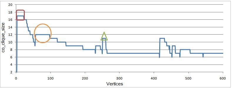
TABLE I
                                                         C OMPARISON E XPERIMENTS

                     Data Sets                           Time Cost (seconds)                         Peak Memory Usage
     Graph Dataset     Vertices      Edges      CSV      TriDN    BiTriDN      T-K-Core      CSV      TriDN    BiTriDN     T-K-Core
       Synthetic          60          308       0.043    0.0012    0.0011       0.0010     1920 KB   1428 KB   1436 KB     1440 KB
        Stocks           242          522       0.041    0.0017    0.0013       0.0012     2760 KB   1532 KB   1540 KB     1552 KB
          PPI           4741        15147        2.51     0.211     0.121        0.097    19000 KB   7988 KB   8224 KB     8244 KB
        DBLP            6445        11848        1.47     0.062     0.046        0.034     8800 KB   8044 KB   8232 KB     8272 KB
     Astro-Author       17903       196972     17393.7    73.8       7.79        1.03       187MB    180 MB    183 MB      182 MB
       Epinions         75879       405741         -     262.13     15.71        4.09          -     282 MB    289 MB      285 MB
       Amazon          262111       899792         -      34.9      10.59        3.81          -     570 MB    584 MB      577 MB
         Wiki          176265      1010204         -      435.8     17.15        7.89          -     677 MB    693 MB      684 MB
         Flickr       1,715,255   15,555,041       -        -    *60 hours        747          -         -        -         2.5 GB
      LiveJournal     4,847,571   42,851,237       -        -          -          443          -         -        -         6.9 GB

upperbound of λ(e), denoted as λ̃(e). In graph G we assign             for BiTriDN is taken from[4], to give the reader a ballpark
λ̃(e) as κ(e) for every edge e.                                        figure – the machine they used had a comparable processor
   Next we prove κ(e) is valid λ̃(e). For edge e(u, v), as-            but with larger memory. The reason for this high processing
sume its maximum Triangle K-Core is subgraph Ge . For any              time for BiTriDN on Flickr dataset is that each iteration is
△(u, v, w) containing e in Ge , according to Theorem 1, we             expensive (55 min per iteration) and a number of iterations (66
have κ(v, w) ≥ κ(e), κ(u, w) ≥ κ(e), so λ̃(v, w) ≥ λ̃(e) ,             are needed for convergence[4]). Compared with DN-Graph,
λ̃(u, w) ≥ λ̃(e). According to Definition 5, vertex w supports         Triangle K-Core allows for a simpler abstraction and this in
λ̃(e). There are at least κ(e) triangles containing edge e in          turns allows us to avoid the iterative approach discussed in
Ge , so there are at least κ(e) vertices supporting λ̃(e). λ̃(e)=      DN-Graph. This is the rationale for the significant speedup
κ(e), therefore λ̃(e) is valid, and κ(e) which equals λ̃(e) is         over DN-Graph variants enabling our algorithm to scale to
valid λ̃(e).                                                           very large datasets. Also, the peak memory usage of Triangle
   The advantage of our algorithm is, we avoid the com-                K-Core algorithm and DN-Graph variants are almost the same,
plex iterative approach suggested in DN-Graph, and yield               and are less than that of CSV.
the speedups. Also, DN-Graph does not discuss the use of                  Second, when comparing our results with CSV plots on the
template pattern cliques, and its incremental method is costly         qualitative visual assessment (Figure 4), we observe that while
since it is iterative.                                                 the order in which vertices are processed may on occasion
                                                                       be slightly different – due to the differences in the estimation
                       VII. E XPERIMENTS
                                                                       procedure of co clique size and resulting in a shift of the main
   In this section we present our experimental results. All ex-        trends – the main trends themselves are quite similar and easy
periments, unless otherwise noted, are evaluated on a 3.2GHz           to discern. In CSV[2], they illustrate the benefit of using the
CPU, 16G RAM Linux-based system at the Ohio Supercom-                  approximate cliques detected by CSV as preprocessing results
puter Center (OSC). The main datasets we evaluated our                 for detecting exact cliques, we can easily see that Triangle
results on can be found in Table I.                                    K-Cores can be used for the same purpose.
A. Comparison with CSV and DN-Graph                                    B. Protein-Protein Interaction (PPI) Case Study
   In our first set of experiments we compare the performance             We also do a case study on PPI network, the plot is in
of Triangle K-Core algorithm (Algorithm1) with CSV[2] and              Figure 5(a). The 3 red circles in the plot indicate 3 approx-
DN-Graph variants (TriDN and BiTriDN (an improvement                   imate cliques, we draw the 3 cliques (from left to right) in
over TriDN))[4] both in terms of efficiency and efficacy.              Figure 5(b)(c)(d). We find that clique 1 is exactly the same as
As noted in Section VI we can theoretically show that the              what Wang et al. detected in [4]. The names in the parenthesis
DN-Graph variants (TriDN and BiTriDN) converge to the                  are the names used in [4]. Clique 2 is shown to be 10-vertex
same value as Algorithm 1. Table I documents the execu-                clique in the plot, in fact it is an exact 10-vertex clique. Clique
tion time/peak memory usage of these algorithms on various             3 has 10 vertices, but it is shown to be 9-vertex clique, because
datasets, while Figure 4 conveys a qualitative comparison by           the edge between APC4 and CDC16 is missed.
realizing the density plots produced by each algorithm (note
that since DN-Graph and Triangle K-Core converge to the                C. Experimental Results of Update Algorithm
same values the density plots are identical).                             To evaluate the effectiveness of our update algorithm we
   First, for all the datasets it is clear that Triangle K-Core        randomly add/delete about 1% of edges from five large
is the fastest to finish. For some large datasets we could             datasets in Table I, and in Table II we compare the time costs
not run BiTriDN or TriDN due to memory thrashing issues                of re-computing and updating the maximum Triangle K-Cores
and CSV was taking too long to terminate. For Flickr and               incrementally. Results reported are averaged over 5 runs. Here
LiveJournal datasets, we execute Triangle K-Core Algorithm 1           Re-compute time is actually the execution time of steps 8-
without storing edges’ triangles in memory. The Flickr result          18 in Algorithm 1, and Update time is the execution time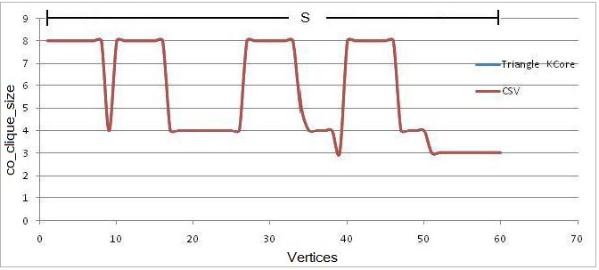
(a) PPI clique distribution

                              (a) Synthetic Dataset

                                                                                                                 (b) PPI clique 1

                               (b) Stocks Dataset

                                                                                                                 (c) PPI clique 2

                            (c) Astro-Author Dataset

                                                                                                                 (d) PPI clique 3
                                                                                                       Fig. 5.    Cliques in PPI dataset

                                 (d) PPI Dataset
                                                                                                                TABLE II
                                                                                                U PDATE A LGORITHM T IME C OST ( SECONDS )

                                                                                        Graph        Total Edges        Edges        Re-compute   Update
                                                                                                                        Changed
                                                                                     Astro-Author    196972             1814             0.27     0.005
                                                                                      Epinions       405741             3953             0.70      0.06
                                                                                       Amazon        899792             7958             0.61      0.01
                                                                                        Flickr       15,555,041         14996            561       1.4
                                                                                     LiveJournal     42,851,237         41996            306       2.4

                                (e) DBLP Dataset

Fig. 4. Qualitative Comparison between CSV and Triangle K-Core Note
that in the figure we note regions in the plot where the two plots are near        of the Algorithm 2. The results clearly demonstrate that the
identical or similar (S) and regions where there is a distinct phase shift (PS).   incremental algorithm is effective.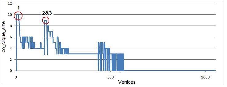
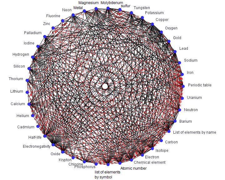
D. Dual View Plots: Wiki Case Study
   In Figure 6, we present an example to illustrate how Dual
View Plots can highlight the change of clique-like structures
within a dynamic graph setting.
   We use two consecutive snapshots of Wiki datasets for
this purpose. A snapshot of Wiki dataset is comprised of
vertices, which are Wiki articles, and references among them.
Figure 6(a) represents the clique distribution plot of 1st
                                                                   (a) Distribution of original cliques in Ga (Plot(a))
snapshot Ga , and it corresponds to plot(a) in Algorithm 3.
Figure 6(b) visualizes the cliques containing new edges in the
2nd snapshot, and it corresponds to plot(b) in Algorithm 3.
   Then in Figure 6(b) we select the 3 cliques with highest
density for more analysis – denoted using a green triangle,
a red rectangle, and an orange ellipse. The Dual View Plot
tool can then locate their corresponding vertices in Figure 6(a)
using the same markers, allowing the user to gain insights
into how these clique-like structures evolved. For example,
one can observe that the vertices (green triangle) are located       (b) Distribution of new cliques in Gb (Plot(b))
in two places in Figure 6(a); some vertices are in a 10-vertex
clique, and one single vertex is in a 5-vertex clique. Drilling
down as shown in Figure 6(c), “Astrology” is the single
vertex, the red dashed-lines are newly added edges. Essentially
between two consecutive snapshots, a new Wiki page and the
corresponding Wiki links were established thereby forming
a larger clique. The details about the other 2 clique-like
structures are presented Figure 6(d) and Figure 6(e) and are                 (c) Clique details (green triangle)
also self explanatory – the two cliques are formed by merging
vertices from different original cliques, they both indicate an
expanding trend on specific topics.
E. Dynamic Template Pattern Cliques: DBLP Study
   The DBLP graph data set is consisted of authors(vertices)
and their collaborations(edges) in each year. In the following
we will detect the template pattern cliques introduced in
Figure 3 in DBLP data set, and show that such cliques reveal
interesting hidden information about paper topics.
   To illustrate the Emerging Clique, we use the DBLP 2003
and 2004 data as two snapshots. Emerging Clique Plot for
DBLP in 2004 is shown in Figure 7. The red circle highlights                     (d) Clique details (red rectangle)
the densest (6-vertex) Emerging Clique. The authors are Rudi
Studer, Karl Aberer, Arantza Illarramendi, Vipul Kashyap,
Steffen Staab, Luca De Santis. They are from 5 different
countries, and they collaborated for the first time in 2004.
   In a similar manner we use DBLP 2003 and 2004 to plot the
Bridge Clique distribution of DBLP 2004 in Figure 8. The first
major clique on the plot (red circle) is an interesting 6-vertex
Bridge Clique. In 2003, the 6 authors were in two independent
groups: Group 1: Divesh Srivastava, Graham Cormode, S.
Muthukrishnan, Flip Korn; and Group 2: Theodore Johnson,
Oliver Spatscheck. In Group 1, the authors primarily worked
on data streams, and in Group 2 the researchers mainly worked
on networking in 2003. In 2004, the 6 authors worked together
on “Holistic UDAFs at Streaming Speeds”, which is a topic
“merged” by data stream and network.
   Using datasets DBLP 2000 and DBLP 2001, we plot the
Expanding Cliques in DBLP 2001 in Figure 9. The densest
                                                                             (e) Clique details (orange ellipse)
                                                                   Fig. 6.    Dual View Plots for Clique Changes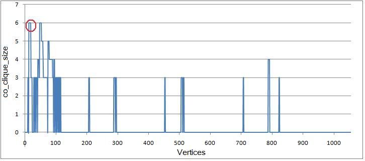
(a) Plot of Bridge Cliques in PPI dataset
           Fig. 7.    Plot of Emerging Cliques in DBLP 2004

                                                                                          (b) Details of Bridge Clique 1
            Fig. 8.    Plot of Bridge Cliques in DBLP 2004
                                                                               Fig. 10.   Detect Bridge Cliques in PPI dataset

                                                                     •   20S proteasome complex: PRE1
                                                                     •   19/22S regulator complex: RPN11, RPN12, RPN9,
                                                                         RPT1, RPN5, RPN5, RPT3, RPN8
                                                                   In Figure 10(b), we draw the details of Bridge Clique 1 in the
                                                                   dashed-line rectangle, where the green vertices belong to the
                                                                   complex “19/22S regulator”, the blue vertices belong to com-
          Fig. 9.     Plot of Expanding Cliques in DBLP 2001       plex “20S proteasome”, black edges are intra-complex edges,
                                                                   red dashed-lines are inter-complex edges. Besides drawing
                                                                   Bridge Clique 1, we also draw other vertices in complex “20S
Expanding Clique (denoted by a red circle) shows a 9-vertex        proteasome”, and find that the vertex “PRE1” is an important
clique. In 2000, the 3 authors Quan Wang, David Maier,             bridge node connecting the two complexes.
Leonard D. Shapiro worked on a paper about Query Pro-                 The proteins in right red circle comprise two Bridge Cliques,
cessing. In 2001, the 3 authors were joined by 6 other authors     the first is Bridge Clique 2:
who did not appear in DBLP 2000 dataset, Paul Benninghoff,            • Gac1p/Glc7p complex: GLC7
Keith Billings, Yubo Fan, Kavita Hatwal, Yu Zhang, Hsiao-             • mRNA cleavage and polyadenylation specificity factor
min Wu, and they worked on one paper “Exploiting Upper                   complex: PAP1, CFT2, CFT1, PTA1, MPE1, YSH1,
and Lower Bounds in Top-Down Query Optimization”, which                  YTH1, REF2
is an extension of the previous work in 2000.
                                                                      the second is Bridge Clique 3:
F. Static Template Pattern Cliques: PPI Case Study                    • mRNA cleavage factor complex: RNA14
   We next discuss how domain-driven template pattern                 • mRNA cleavage and polyadenylation specificity factor
cliques based on Triangle K-Cores can be exploited in the                complex: PAP1, CFT2, CFT1, PTA1, MPE1, YSH1,
case of static data such as Protein Protein Interaction (PPI)            YTH1, FIP1
data. In PPI dataset, each vertex represents a protein, and        We find that Bridge Clique 2 and 3 have a lot of overlap
each protein belongs to a complex, which includes proteins of      vertices, which indicate that all the vertices in them are very
similar functions. Now we define a variant of Bridge Clique to     closely related in function, this is consistent with known
be a clique that connects vertices from two different complexes.   biological knowledge..
Here we define an edge’s label to be “new” when it connects
two vertices from different complexes, otherwise its label is                             VIII. C ONCLUSIONS
“old”. Then we apply the previously described Bridge Clique           In this paper, we introduce the notion of a Triangle K-Core,
detection algorithm on PPI dataset, and get the Bridge Clique      a simple topological motif and demonstrate how to extract such
distribution plot in Figure 10(a).                                 structures efficiently from both static and dynamic graphs. We
   We highlight two peaks using red circles, the Bridge Clique     empirically demonstrate on a range of real-world data that
1 in left red circle is comprised of vertices from the following   this motif can be used as a proxy for probing and visualizing
two complexes:                                                     relevant clique-like structure from large dynamic graphs and
networks. Finally, we discuss a method to extend the basic [23] P. Papadimitriou, A. Dasdan, and H. Garcia-Molina, “Web graph sim-
definition to support user defined clique template patterns with ilarity for anomaly detection,” Proceeding of the 17th international
conference on World Wide Web, 2008.
applications to network visualization, correspondence analysis
and event detection on graphs and networks. IX. A PPENDIX
ACKNOWLEDGMENT A. Triangle K-Core Update Algorithm
We thank Dave Fuhry, Ye Wang and the anonymous re- Before executing the update algorithm, for each edge e, we
viewers for many helpful suggestions for improving this work. firstly initialize e.order, which indicates the time when e is
We also thank the authors of [4] for sharing their code base. processed in Algorithm 1. If e.order is less than e’.order, then
Aspects of this work was supported under the following NSF e is processed earlier than e’. After execution of Algorithm 1
grants: IIS0917070 and IIS1141828. e.order is initialized as the index of edge e in list Edges.
R EFERENCES Algorithm 5 Update Algorithm for Adding Edges
[1] U. Feige, S. Goldwasser, L. Lovasz, S. Safra, and M. Szegedy, “Ap- 1: for each added triangle tnew do
proximating Clique is Almost NP-Complete,” FOCS, 1991. 2: Create empty lists ChangingList, PotentialList, TempList;
[2] N. Wang, S. Parthasarathy, K.-L. Tan, and A. K. H. Tung, “CSV: 3: Find the smallest value µ of tnew ’s edges’ κ value;
Visualizing and Mining Cohesive Subgraphs,” ACM SIGMOD, 2008. 4: Put tnew ’s edges whose κ value equals µ in PotentialList in
[3] M. Ankerst, M. M. Breunig, H.-P. Kriegel, and J. Sander, “OPTICS: order;
ordering points to identify the clustering structure,” ACM SIGMOD,
5: AddToCore(tnew , e0 ); // e0 is the first edge of PotentialList
1999.
[4] N. Wang, J. Zhang, K. Tan, and A. K. H. Tung, “On Triangulation-based 6: κ(e0 ) + +;
Dense Neighborhood Graphs Discovery,” PVLDB, 2010. 7: for each edge e in PotentialList do
[5] A. Y. Ng, M. I. Jordan, and Y. Weiss, “On Spectral Clustering: Analysis 8: ori κ(e) = µ;
and an algorithm,” Advances in Neural Information Processing Systems, 9: Construct triangles set e.addTris;
vol. 14, 2001. 10: for each triangle ta in e.addTris do
[6] V. Satuluri and S. Parthasarathy, “Scalable Graph Clustering Us- 11: AddToCore(ta , e);
ing Stochastic Flows: Applications to Community Discovery,” ACM 12: κ(e) + +;
SIGKDD, 2009. 13: Construct triangles set e.delTris;
[7] G. Karypis and V. Kumar, “A Fast and High Quality Multilevel Scheme 14: for each triangle td in e.delTris do
for Partitioning Irregular Graphs,” SIAM Journal on Scientific Comput-
ing, vol. 20, 1998.
15: if κ(e) > ori κ(e) then
[8] I. Dhillon, Y. Guan, and B. Kulis, “A Fast Kernelbased Multilevel 16: DelFromCore(td , e);
Algorithm for Graph Clustering,” ACM SIGKDD, 2005. 17: κ(e) − −;
[9] M. R. Garey and D. S. Johnson, Computers and Intractability: A Guide 18: Remove e from PotentialList;
to the Theory of NP-Completeness. San Francisco: W. H. Freeman, 19: if κ(e) > ori κ(e) then
1979. 20: put e to ChangingList;
[10] J. Wang, Z. Zeng, and L. Zhou, “CLAN: An Algorithm for Mining 21: Insert e.post edges to PotentialList in order;
Closed Cliques from Large Dense Graph Databases,” ICDE, 2006. 22: else
[11] J. Abello, M. G. C. Resende, and S. Sudarsky, “Massive Quasi-Clique 23: TempList = Simulate Algo1(e);
Detection,” Proceedings of the 5th Latin American Symposium on
Theoretical Informatics, 2002.
24: Insert edges in TempList between e’s previous and next
[12] Z. Zeng, J. Wang, L. Zhou, and G. Karypis, “Coherent closed quasi- edge in Edges list;
clique discovery from large dense graph databases,” ACM SIGKDD, 25: while ChangingList is not empty do
2006. 26: TempList = Simulate Algo1(ChangingList.min edge);
[13] J. Leskovec, J. Kleinberg, and C. Faloutsos, “Graphs over time: den- 27: Insert edges in TempList in Edges list, between the last edge
sification laws, shrinking diameters and possible explanations,” ACM with κ(e) = µ and first edge with κ(e) = µ + 1;
SIGKDD, 2005.
[14] L. Backstrom, D. Huttenlocher, J. Kleinberg, and X. Lan, “Group
formation in large social networks: membership, growth, and evolution,”
ACM SIGKDD, 2006.
[15] S. Asur, S. Parthasarathy, and D. Ucar, “An event-based framework for Algorithm 6 Simulate Algo1(einit )
characterizing the evolutionary behavior of interaction graphs,” ACM 1: Create an empty list TempList;
TKDD, vol. 3, no. 16, 2009. 2: Add einit to TempList;
[16] J. Sun, C. Faloutsos, S. Papadimitriou, and P. S. Yu, “GraphScope: 3: for each edge e in TempList do
parameter-free mining of large time-evolving graphs,” ACM SIGKDD, 4: Construct triangles set e.addTris;
2007. 5: for each edge e′ that shares a triangle T in e.addTris with e
[17] Y.-R. Lin, Y. Chi, S. Zhu, H. Sundaram, and B. L. Tseng, “Facetnet:a
framework for analyzing communities and their evolutions in dynamic
and e’ is in ChangingList do
networks.” WWW, 2008. 6: if κ(e′ ) > κ(e) then
[18] G. M. Namata, B. Staats, L. Getoor, and B. Shneiderman, “A dual-view 7: DelFromCore(T, e’);
approach to interactive network visualization,” ACM CIKM, 2007. 8: κ(e′ ) − −;
[19] X. Yang, S. Asur, S. Parthasarathy, and S. Mehta, “A Visual-Analytic 9: if κ(e′ ) = κ(e) then
Toolkit for Dynamic Interaction Graphs,” ACM SIGKDD, 2008. 10: Move e’ from ChangingList to TempList;
[20] J. Abello, F. V. Ham, and N. Krishnan, “ASK-GraphView: A Large 11: Return TempList;
Scale Graph Visualization System ,” IEEE TVCG, 2006.
[21] V. Batagelj and M. Zaversnik, “An O(m) Algorithm for Cores Decom-
position of Networks,” CoRR, arXiv.org/cs.DS/0310049, 2003. Algorithm 5 is to update edges’ maximum Triangle K-Cores
[22] Y. Zhang and S. Parthasarathy, “Extracting Analyzing and Visualizing
Triangle K-Core Motifs within Networks,” OSU-CISRC-8/11-TR25, when adding edges. In step 4, according to Rule 0, we put
2011. some edges of tnew in PotentialList because their maximumTriangle K-Cores might change. All edges in PotentialList are Algorithm 7 Update Algorithm for Deleting Edges
sorted in the increasing order of e.order, that is because we will 1: for each deleted triangle tdel do
simulate Algorithm 1 to recompute on PotentialList, we need 2: Create empty lists ChangingList, PotentialList;
3: Find the smallest value µ of tdel ’s edges’ κ value;
to maintain the order. tnew is not yet in any edge’s maximum 4: Put tdel ’s edges whose κ value equals µ in PotentialList in
Triangle K-Core, so in steps 5-6, we add it to the maximum order;
Triangle K-Core of the first edge of PotentialList. 5: for each edge e in PotentialList do
Steps 7-24 update κ(e) for each edge e in PotentialList. In 6: if IsInCore(tdel , e) then
step 8, ori κ(e) stores the original maximum Triangle K-Core 7: DelFromCore(tdel , e);
8: κ(e) − −;
number of e before update, according to Rule 0, this value is 9: for each edge e in PotentialList do
equal to µ. In step 9 we construct the following set of triangles 10: ori κ(e) = µ;
that violate Theorem 1 (IsInCore(t, e) tests whether triangle t 11: Construct triangles sets e.addTris and e.delTris;
is in edge e’s maximum Triangle K-Core): 12: while true do
13: if κ(e) < ori κ(e) then
• e.addTris ={△t | △t is on edge e, and △t con-
14: if e.addTris is not empty then
tains edge e’ that κ(e′ ) > κ(e) ∧ IsInCore(t, e′ ) ∧ 15: AddToCore(e.addTris.first, e);
!IsInCore(t, e)} 16: κ(e) + +;
Steps 10-12 then process these “illegal” triangles in e.addTris. 17: remove e.addTris.first from e.addTris;
18: else
After that, κ(e) might increase and lead to the following set
19: break;
of triangles that violate Theorem 1: 20: if κ(e) = ori κ(e) then
• e.delTris ={△t | △t is on edge e, and △t contains 21: if e.delTris is not empty then
edge e’ that e′ .order < e.order ∧ κ(e′ ) < κ(e) ∧ 22: DelFromCore(e.delTris.first, e);
IsInCore(t, e′ ) ∧ IsInCore(t, e)}, 23: κ(e) − −;
24: remove e.delTris.first from e.delTris;
Steps 14-17 then process these “illegal” triangles in e.delTris. 25: else
In step 19, if κ(e) increases, some of e’s neighbor edges 26: break;
might change κ value, according to Rule 0, these edges are in 27: Remove e from PotentialList;
the following set, 28: if κ(e) < ori κ(e) then
′ 29: Put e in ChangingList;
• e.post edges = {Edge e | e’ shares a triangle with e, and 30: Insert e.share edges to PotentialList in order;
′ ′
κ(e ) = µ ∧ e .order > e.order} 31: Insert edges in ChangingList in Edges list, between the last
we put these edges in PotentialList. edge with κ(e) = µ − 1 and first edge with κ(e) = µ;
If κ(e) does not change, then edge e is processed now, in
step 23 we use method Simulate Algo1 to simulate Algorithm
1 to update e and its neighbors’ maximum Triangle K-Cores. Theorem 1. In steps 28-30, if κ(e) changes, according to Rule
Simulate Algo1 will return a list of edges whose κ value 0 we find the following set of edges whose maximum Triangle
is determined. When all edges in PotentialList have been K-Core might change, and insert them in PotentialList.
′
processed, we update maximum Triangle K-Cores of edges • e.share edges = {Edge e | e’ shares a triangle with e,
′
in ChangingList (step 26), ChangingList.min edge is the edge κ(e ) = µ}
in ChangingList with the minimum κ value. In step 27 we Finally we put the edges in ChangingList in correct positions
put all edges in ChangingList in the corresponding positions in list Edges.
in sorted list Edges. In Algorithm 5 and 7, after each iteration, each edge’s
Algorithm 7 is to update edges’ maximum Triangle K-Cores order value needs to be re-computed, which will be costly.
when deleting edges. In step 4, according to Rule 0, we put In our implementation, we only update edges whose order
some edges of tdel in PotentialList. In steps 5-8, we remove value have been changed, that is, when a set of edges {e1, e2,
deleted triangles from its edges’ maximum Triangle K-Cores. ...en} are inserted between two edges Ea, Eb, then ei.order =
In step 11, we construct two sets of triangles on e: Ea.order + (Eb.order − Ea.order) ∗ i/(n + 1).
• e.addTris = {△t | △t is on edge e, and contains edge If we do not store triangles in Algorithm 1, when updating
e’ that, κ(e′ ) = ori κ(e) ∧ e′ .order < e.order ∧ edge e in PotentialList we need to re-construct e’s triangles,
IsInCore(t, e′ )∧!IsInCore(t, e) } and the triangle information we need to know is whether
• e.delTris = {△t | △t is on edge e, and contains a triangle of e is in e’s maximum Triangle K-Core. We
edge e’ that, κ(e′ ) < ori κ(e) ∧ IsInCore(t, e′ ) ∧ recover this information as following: we firstly get triangle t’s
IsInCore(t, e) } “process time”, which is the smallest order value of its edges,
When step 13 is satisfied, all the triangles in e.addTris then we apply the following Rule to find all e’s triangles in
violate Theorem 1, so we add the first triangle of e.addTris e’s maximum Triangle K-Core.
to e’s maximum Triangle K-Core to obey Theorem 1. Then • Rule 1: if κ(e)=k, then we sort e’s triangles in the in-
κ(e) changes and if now step 20 is satisfied, all the triangles creasing order of their “process time”, the last k triangles
in e.delTris violate Theorem 1, so we remove the first triangle will be in e’s maximum Triangle K-Core.
of e.delTris from maximum Triangle K-Core of e to obey The correctness of Rule 1 is proved in our technical report[22].You can also read