Bias in Knowledge Graph Embeddings
←
→
Page content transcription
If your browser does not render page correctly, please read the page content below
Bias in Knowledge Graph Embeddings

                         A Thesis

               submitted to the designated
                 by the General Assembly
of the Department of Computer Science and Engineering
                 Examination Committee

                            by

                     Styliani Bourli

in partial fulfillment of the requirements for the degree of

  MASTER OF SCIENCE IN DATA AND COMPUTER
                SYSTEMS ENGINEERING

                WITH SPECIALIZATION
        IN DATA SCIENCE AND ENGINEERING

                  University of Ioannina
                      February 2021
Examining Committee:

  • Evaggelia Pitoura, Professor, Department of Computer Science and Engineer-
    ing, University of Ioannina (Advisor)

  • Panos Vassiliadis, Professor, Department of Computer Science and Engineering,
    University of Ioannina

  • Panayiotis Tsaparas, Assoc. Professor, Department of Computer Science and
    Engineering, University of Ioannina
ACKNOWLEDGEMENTS I would like to express my sincere thanks to my advisor, Prof. Evaggelia Pitoura, for the opportunity she gave me to perform this thesis in an interesting field such as the knowledge graph embeddings, as well as for the important help, support and guidance she has provided me.
TABLE OF CONTENTS

List of Figures                                                                             iii

List of Tables                                                                               v

Abstract                                                                                    vii

Εκτεταμένη Περίληψη                                                                         ix

1 Introduction                                                                               1
   1.1   Motivation . . . . . . . . . . . . . . . . . . . . . . . . . . . . . . . . . . .    1
   1.2 Structure . . . . . . . . . . . . . . . . . . . . . . . . . . . . . . . . . . . .     3

2 Preliminaries                                                                              4
   2.1 Knowledge Graph . . . . . . . . . . . . . . . . . . . . . . . . . . . . . .           4
   2.2 Knowledge Graph Embeddings . . . . . . . . . . . . . . . . . . . . . . .              6
   2.3 Knowledge Graph Embedding Models . . . . . . . . . . . . . . . . . . .                7
         2.3.1   The TransE model . . . . . . . . . . . . . . . . . . . . . . . . . .        8
         2.3.2 The TransH model . . . . . . . . . . . . . . . . . . . . . . . . . .          8
         2.3.3 Comparison of the two models . . . . . . . . . . . . . . . . . . .            9
   2.4 Notations . . . . . . . . . . . . . . . . . . . . . . . . . . . . . . . . . . .       9

3 Bias in the dataset                                                                       10
   3.1 Metrics for measuring bias in the dataset . . . . . . . . . . . . . . . . . 10
         3.1.1   Equal opportunity approach . . . . . . . . . . . . . . . . . . . . 10
         3.1.2   Equal number approach . . . . . . . . . . . . . . . . . . . . . . . 11
         3.1.3   Measuring bias in data with the two approaches . . . . . . . . . 11

4 Bias in knowledge graph embeddings                                                        13
   4.1 Methods for measuring bias in knowledge graph embeddings                 . . . . . 13

                                              i
4.1.1 Projection method . . . . . . . . . . . . . . . . . . . . . . . . . . 13
4.1.2 Analogy puzzle method . . . . . . . . . . . . . . . . . . . . . . . 15
4.1.3 Prediction method . . . . . . . . . . . . . . . . . . . . . . . . . . 16
4.2 Clustering fairness using knowledge graph embeddings . . . . . . . . . 16
4.2.1 Clustering fairness using knowledge graph embeddings . . . . . 17
5 Debias the knowledge graph embeddings 18
5.1 Debias approach . . . . . . . . . . . . . . . . . . . . . . . . . . . . . . . 18
6 Experiments 20
6.1 Datasets . . . . . . . . . . . . . . . . . . . . . . . . . . . . . . . . . . . . 20
6.1.1 Synthetic knowledge graph . . . . . . . . . . . . . . . . . . . . . 21
6.1.2 Real knowledge graphs . . . . . . . . . . . . . . . . . . . . . . . 21
6.1.3 Training the knowledge graphs . . . . . . . . . . . . . . . . . . . 23
6.2 Bias in the dataset . . . . . . . . . . . . . . . . . . . . . . . . . . . . . . 23
6.2.1 Data bias metric selection . . . . . . . . . . . . . . . . . . . . . . 24
6.2.2 Bias results in the datasets . . . . . . . . . . . . . . . . . . . . . 27
6.3 Bias results in the KG embeddings . . . . . . . . . . . . . . . . . . . . . 31
6.3.1 Bias results in the KG embeddings using projections . . . . . . . 31
6.3.2 Detection of bias in KG embeddings using an analogy puzzle . . 36
6.3.3 Prediction task for bias amplification detection . . . . . . . . . . 38
6.4 Clustering results . . . . . . . . . . . . . . . . . . . . . . . . . . . . . . . 42
6.5 Debias evaluation . . . . . . . . . . . . . . . . . . . . . . . . . . . . . . . 47
6.5.1 Evaluation using projections and similarity . . . . . . . . . . . . 47
6.5.2 Evaluation using prediction task . . . . . . . . . . . . . . . . . . 49
6.5.3 Evaluation using clustering . . . . . . . . . . . . . . . . . . . . . 52
7 Related Work 55
8 Conclusions and Future work 57
Bibliography 58
iiLIST OF FIGURES
2.1 Example of a knowledge graph. . . . . . . . . . . . . . . . . . . . . . . 5
2.2 Example of KG embeddings representation in the 2-dimensional vector
space. . . . . . . . . . . . . . . . . . . . . . . . . . . . . . . . . . . . . . 7
2.3 If (‘‘M ona Lisa”, ‘‘was created by”, ‘‘Leonardo da V inci”) triple holds,
then using Transe model ‘‘M ona ⃗ Lisa” + ‘‘was created
⃗ by” should be
near to ‘‘Leonardo⃗ da V inci” and using TransH model, ‘‘M ona⃗ Lisa⊥ ”+
⃗
‘‘was created by” should be near to ‘‘Leonardo⃗da V inci⊥ ”. . . . . . . . 9
6.1 There is a power law distribution on the number of individuals per
occupation in both the original graph and the subgraph; there are few
occupations that many users have and many that few have. . . . . . . 22
6.2 Average results of prediction task using five synthetic graphs and TransE
embeddings. . . . . . . . . . . . . . . . . . . . . . . . . . . . . . . . . . 27
6.3 Average results of prediction task using five synthetic graphs and TransH
embeddings. . . . . . . . . . . . . . . . . . . . . . . . . . . . . . . . . . 28
6.4 Plots of the distribution of neutral occupations for different values of
t. The 6.4a refers to Wikidata subgraph and the gender sensitive
attribute. The appopriate value for t is 0.0001. The 6.4b refers to FB13
dataset and the religion sensitive attribute. The appropriate value for t
is 0.001. The 6.4c refers to FB13 dataset and the nationality sensitive
attribute. The appropriate value for t is also 0.001. The 6.4d refers
to FB13 dataset and the enthnicity sensitive attribute. The appropriate
value for t is here 0.01. . . . . . . . . . . . . . . . . . . . . . . . . . . . 30
iii6.5 Let a, b be the sensitive values. Then the upper right box of each plot
refers to the occupations characterized as a both in data and in the
embeddings. The bottom right box refers to the occupations marked as
a in the data and b in the embeddings. The lower left box refers to the
occupations marked as b both in data and in the embeddings. Finally,
the upper left box refers to the occupations marked as b in the data,
but as a in the embeddings. . . . . . . . . . . . . . . . . . . . . . . . . . 35
6.6 The expected and the predicted numbers of individuals in top-K results
using TransE embeddings. Gender concerns to Wikidata dataset, while
religion, nationality and ethnicity concern to FB13 dataset. . . . . . . . 39
6.7 The expected and the predicted numbers of individuals in top-K results
using TransH embeddings. Gender concerns to Wikidata dataset, while
religion, nationality and ethnicity concern to FB13 dataset. . . . . . . . 40
6.8 Clustering results using FB13 dataset and TransE embeddings. . . . . . 43
6.9 Clustering results using FB13 dataset and TransH embeddings. . . . . . 44
6.10 Clustering results of occupations using FB13 dataset and TransE em-
beddings. . . . . . . . . . . . . . . . . . . . . . . . . . . . . . . . . . . . 45
6.11 Clustering results of occupations using FB13 dataset and TransH em-
beddings. . . . . . . . . . . . . . . . . . . . . . . . . . . . . . . . . . . . 46
6.12 Prediction task for debias evaluation using λ=0.5, λ=0.8 and K=10. . . 51
6.13 Clustering results of occupations using TransE embeddings before de-
bias and after a debias with λ=0.8. . . . . . . . . . . . . . . . . . . . . . 53
6.14 Clustering results of occupations using TransH embeddings before de-
bias and after a debias with λ=0.8. . . . . . . . . . . . . . . . . . . . . . 54
ivLIST OF TABLES
6.1 Information of the real datasets. . . . . . . . . . . . . . . . . . . . . . . 23
6.2 Information about the number of individuals and occupations of each
sensitive attribute in the datasets. The gender sensitive attribute con-
cerns the Wikidata subgraph, while the religion, nationality and eth-
nicity sensitive attributes concern the FB13. . . . . . . . . . . . . . . . . 29
6.3 The five most biased occupations based on gender, religion, nationality
and ethnicity sensitive attributes on Wikidata subgraph and FB13 dataset. 29
6.4 The five most biased occupations based on gender, religion, national-
ity and ethnicity sensitive attributes on Wikidata subgraph and FB13
dataset. In Table 6.4a there are the results from TransE embeddings,
while in Table 6.4b there are the results from TransH embeddings. . . 32
6.5 Pearson correlation coefficient score between data bias and embedding
bias using TransE and TransH embeddings. . . . . . . . . . . . . . . . . 33
6.6 Pearson correlation coefficient score between popularity and embedding
bias using our metric, let be proj, the embedding bias metric in [1] and
the FB13 dataset. . . . . . . . . . . . . . . . . . . . . . . . . . . . . . . . 34
6.7 Percentage of occupations, which are characterized as a or b both in the
dataset and in the embeddings. . . . . . . . . . . . . . . . . . . . . . . . 36
6.8 The pairs of occupations that suit in the analogy puzzle “b is to x as a
is to y”, where a and b are two sensitive values. . . . . . . . . . . . . . 37
6.9 Quantification of amplification. The average results of the predicted −
expected score of the five most biased occupations, using TransE em-
beddings, K=10, 20, 50, 100 for the Wikidata subgraph (for gender),
and K = 5, 7, 10 for FB13 dataset (for religion, nationality and ethnicity). 41
v6.10 Quantification of amplification. The average results of the predicted −
expected score of the five most biased occupations, using TransH em-
beddings, K=10, 20, 50, 100 for the Wikidata subgraph (for gender),
and K = 5, 7, 10 for FB13 dataset (for religion, nationality and ethnicity). 41
6.11 Results of the semantic relation of occupations in the clusters. . . . . . 47
6.12 Let a, b be the two sensitive values. Table 6.12a gives the average pro-
jection score results of a, b and neutral occupations on bias direction
using TransE embeddings. Moreover Table 6.12b gives the average pro-
jection score results of a, b and neutral occupations on bias direction
using TransH embeddings. Both Tables present the projection score be-
fore debias, after a “soft” debias with λ=0.5 and after a “hard” debias
with λ=1. . . . . . . . . . . . . . . . . . . . . . . . . . . . . . . . . . . . 48
6.13 Let a, b be the two sensitive values. Table 6.13a gives the average cosine
similarity results of a, b and neutral occupations with a and b entities
using TransE embeddings. Moreover Table 6.13b gives the average
cosine similarity results of a, b and neutral occupations with a and
b entities using TransH embeddings. Both Tables present the cosine
similarity score before debias, after a “soft” debias with λ=0.5 and
after a “hard” debias with λ=1. . . . . . . . . . . . . . . . . . . . . . . . 50
6.14 Hits@10 for the most 40 biased gender occupations using Wikidata
dataset, and Hits@5 for the most 20 biased religion, nationality and
ethnicity occupations using FB13 dataset. . . . . . . . . . . . . . . . . . 52
viABSTRACT
Styliani Bourli, M.Sc. in Data and Computer Systems Engineering, Department of
Computer Science and Engineering, School of Engineering, University of Ioannina,
Greece, February 2021.
Bias in Knowledge Graph Embeddings.
Advisor: Evaggelia Pitoura, Professor.
Knowledge graphs (KGs) are multi-relational directed graphs used in many tasks
in recent years, including question answering, recommendation and information re-
trieval. They are associated with, and used by search engines such as Google, Bing,
and Yahoo; and social networks such as LinkedIn and Facebook. Knowledge graph
embeddings have gained a lot of attention recently, because they can map the compo-
nents of a knowledge graph to a low dimensional vector space. In the era of big data,
this is very important because it makes KG usage and analysis easier. But the con-
nection of the KG embeddings production with machine learning, combined with the
fact that bias learning problem using machine learning tasks receives more attention
in current research, leads to concern about bias that may exists in data, transferred to
the KG embeddings through learning and possibly reinforced by them. In this thesis
we study the bias in KG embeddings.
We first define two approaches to quantify the bias in the dataset and after their
comparison we choose the one we consider more appropriate. For measuring bias in
the KG embeddings, we use a projection method and an analogy puzzle to determine
quantitatively and qualitatively if the bias is transferred from the data to the KG
embeddings. We also apply a prediction method to study if there is in addition a
bias amplification using the KG embeddings. We further detect if the popularity of
some entities, or the inequality in populations of sensitive values like male, female
individuals in the dataset, affects bias in KG embeddings, and, moreover, if other
tasks such as clustering affected by the bias of the KG embeddings. We then define a
viidebias method based on projections in the bias subspace. Its novelty lies on tuning
the amount of bias it removes and in the usage of pretrained embeddings instead of
the modification of the KG embedding model.
We conduct experiments using a set of real and synthetic KGs and two widely
known KG embedding models. We provide a presentation and an analysis of the
results. Our approaches can be easily generalized in other datasets and more KG
embedding models.
viiiΕΚΤΈΤΆμΈΝΉ ΠΈΡΊΛΉΨΉ
Στυλιανή Μπουρλή, Δ.Μ.Σ. στη Μηχανική Δεδομένων και Υπολογιστικών Συστημά-
των, Τμήμα Μηχανικών Η/Υ και Πληροφορικής, Πολυτεχνική Σχολή, Πανεπιστήμιο
Ιωαννίνων, Φεβρουάριος 2021.
Μεροληψία σε Ενσωματώσεις Γραφημάτων Γνώσης.
Επιβλέπων: Ευαγγελία Πιτουρά, Καθηγήτρια.
Τα γραφήματα γνώσης (knowledge graphs), είναι κατευθυνόμενα γραφήματα
που περιέχουν πληροφορία διαφόρων οντοτήτων και σχέσεων του πραγματικού κό-
σμου. Χρησιμοποιούνται σε πολλές εφαρμογές τα τελευταία χρόνια, όπως στην
ανάκτηση πληροφορίας και σε συστήματα συστάσεων, καθώς επίσης σε μηχανές
αναζήτησης, όπως Google, Bing και Yahoo, αλλά επίσης και σε κοινωνικά δίκτυα,
όπως το LinkedIn και το Facebook. Μερικά από τα μεγαλύτερα γραφήματα γνώ-
σης είναι της Microsoft, του ebay, της Google και του Facebook. Υπάρχουν όμως
και ανοικτά γραφήματα ελεύθερης πρόσβασης όπως το Wikidata ή παλιότερα το
Freebase.
Οι ενσωματώσεις γραφημάτων γνώσεις (knowledge graph embeddings), έχουν
συγκεντρώσει μεγάλο ενδιαφέρον τα τελευταία χρόνια, επειδή μπορούν και ανα-
παριστούν την πληροφορία των γραφημάτων γνώσης με διανύσματα σε ένα χώρο
χαμηλής διάστασης. Δεδομένου του ότι ζούμε στην εποχή των μεγάλων δεδομένων, η
αναπαράσταση της πληροφορίας με διανύσματα και μάλιστα σε έναν χαμηλής διά-
στασης διανυσματικό χώρο, βοηθάει στην ευκολότερη διαχείριση και ανάλυση των
γραφημάτων. Όμως, το γεγονός ότι η παραγωγή των ενσωματώσεων είναι άμεσα
συνδεδεμένη με την εφαρμογή μηχανικής μάθησης στο γράφημα, σε συνδυασμό με
το πρόβλημα που έχει εντοπιστεί τα τελευταία χρόνια μεταφοράς πληροφορίας με-
ροληψίας μέσω της μάθησης, οδηγεί σε ανησυχία για πιθανή μετάδοση πληροφορίας
που σχετίζεται με τη μεροληψία στις ενσωματώσεις, και ίσως σε ενίσχυσή της από
ixαυτές κατά τη χρήση τους. Σε αυτή την εργασία, μελετάμε συγκεκριμένα τη μερο-
ληψία στις ενσωματώσεις των γραφημάτων γνώσης.
Όσον αφορά τα δεδομένα στο γράφημα αναμένουμε ότι, εφόσον προέρχονται
από την πραγματική ζωή στην οποία υπάρχει συχνά ανισότητα και αδικία, η πλη-
ροφορία που έχουν περιέχει μεροληψία. Για να εξακριβώσουμε αν αυτό όντως συμ-
βαίνει, αλλά και να μετρήσουμε την μεροληψία αυτή στα δεδομένα, ορίζουμε δύο
μετρικές. Μετά από σύγκριση των δύο μετρικών επιλέγουμε αυτή που θεωρούμε
καταλληλότερη. Στη συνέχεια, για να εξετάσουμε αν η μεροληψία μεταφέρεται από
τα δεδομένα στις ενσωματώσεις, αλλά και για να μετρήσουμε ποσοτικά και ποιο-
τικά τη μεροληψία αυτή, χρησιμοποιούμε δύο μεθόδους, μία μέθοδο βασισμένη σε
προβολές και ένα παζλ βασισμένο σε αναλογίες. Ωστόσο ενδιαφερόμαστε επιπλέον
εκτός από το να εντοπίσουμε αν η μεροληψία μεταδίδεται στις ενσωματώσεις, αν
ενδεχομένως ενισχύεται από αυτές, για αυτό και χρησιμοποιούμε μία μέθοδο βα-
σισμένη σε πρόβλεψη. Μια ακόμα ενδιαφέρουσα μελέτη που κάνουμε είναι όσον
αφορά τη σχέση της δημοφιλίας και της ανισότητας στον πληθυσμό δύο ευαίσθητων
τιμών, όπως αντρών – γυναικών στα δεδομένα, με τη μεροληψία στις ενσωματώσεις,
αλλά και αν άλλες εφαρμογές όπως η συσταδοποίηση επηρεάζονται από τη μερεο-
ληψία αυτή. Επειδή τα αποτελέσματα επιβεβαιώνουν την ανησυχία μας όσον αφορά
τη μεροληψία και επειδή οι ενσωματώσεις των γραφημάτων γνώσης χρησιμοποιού-
νται ευρέως σε πολλές σημαντικές εφαρμογές, κρίνουμε στη συνέχεια αναγκαίο
τον ορισμό μίας μεθόδου αφαίρεσης της πληροφορίας αυτής από τα διανύσματα.
Η καινοτομία του έγκειται στη δυνατότητα επιλογής της ποσότητας της μερολη-
ψίας που αφαιρείται και στη χρήση προ-εκπαιδευμένων ενσωματώσεων αντί της
τροποποίησης του μοντέλου παραγωγής τους.
Για να εξετάσουμε αν ισχύουν οι ισχυρισμοί μας, αλλά και για να αξιολογή-
σουμε τις μεθόδους μας χρησιμοποιούμε δύο πολύ γνωστά γραφήματα γνώσεων, το
Wikidata και το FB13, και ένα σύνολο από συνθετικά γραφήματα. Χρησιμοποιούμε
επιπλέον ενσωματώσεις που παράγουμε μέσω δύο διάσημων μοντέλων, του TransE
και του TransH. Στην εργασία παρουσιάζουμε αναλυτικά όλα τα αποτελέσματα
και τα συμπεράσματα από τα πειράματα μας. Είναι σημαντικό ότι οι μέθοδοι που
προτείνουμε μπορούν εύκολα να επεκταθούν και να χρησιμοποιηθούν και σε άλλα
γραφήματα, και σε ενσωματώσεις παραγόμενες από άλλα μοντέλα.
xCHAPTER 1
INTRODUCTION
1.1 Motivation
1.2 Structure
1.1 Motivation
In the era of big data, knowledge graph embeddings are gaining more and more
interest in the scientific world, as they can represent complex data using vectors of
low dimension. Knowledge graph embeddings come from knowledge graphs (KG),
that are multi-relational directed graphs widely used to represent knowledge of real-
world entities in the form of triples. Each edge represents a specific relation between
the two entities (nodes) it connects. Knowledge graphs are used in many applications
including question answering, recommendation and information retrieval. They used
also by famous search engines and social networks, such as Google and Facebook.
KG embeddings map the components of a knowledge graph, such as its entities and
relations, to some low dimensional vector space (e.g., [2, 3, 4]). They have gained
a lot of attention, since they are useful in a variety of tasks such as KG completion
and relation extraction. Furthermore, vector operations are simpler and faster than
the corresponding operations on graphs.
But there is a connection of the embeddings production with machine learning
tasks. This combined with the fact that as machine learning algorithms are increas-
ingly being used, concerns about unfairness and bias in the treatment of sensitive
1attributes are raised (see e.g., [5] for a survey), leads to worry about bias that may
exists in data, transferred to the embeddings through machine learning and possibly
reinforced by them. A recent work in word embeddings has shown that they encode
various forms of social biases [6]. Bias is, generally, disproportionate weight in favor
of or against an idea or thing and can have devastating effects on link prediction
or recommendation systems. It could make easiest for a system to consider that a
man has as occupation the occupation ”computer programmer” for example, than
a woman, or depict mostly males in Google’s image search for ”CEO” [7]. So, as
embeddings are used in various important applications, it is important to discover if
they contain biases.
In this thesis we study bias in KG embeddings. More specifically, we start by
proposing two metrics for measuring bias in the dataset. Since in most cases, knowl-
edge comes from the real world, it is expected to reflect existing social biases [8, 9].
After the comparison of the metrics, we choose the one we consider more appropriate.
Then we define a method based on projections and an analogy puzzle, to determine
quantitatively and qualitatively if the bias is transferred from the data to the KG
embeddings. In contrast with [1] analysis, we measure the bias in the data and com-
pare it with the bias in the KG embeddings, we propose a method to measure the
bias in KG embeddings, that is more simple and efficient, and it is also include the
information of popularity of the entities we are interested in, such as occupations.
We also study if the bias not only transferred to the KG embeddings, but also if it is
amplified by them and if the inequality in populations of the sensitive values affects
the bias. We then apply a prediction method to study if there is in addition a bias
amplification using the KG embeddings. We further detect if the popularity of some
entities, or the inequality in populations of sensitive values like male, female individ-
uals in the dataset, affects bias in KG embeddings, and, moreover, if other tasks such
as clustering is affected by the bias of the KG embeddings. Finally, we propose our
debias approach for removing gender bias in occupation embeddings. In relation to
[10], its novelty lies on tuning the amount of bias it removes using pretrained embed-
dings instead of modifying the KG embedding model and on removing information
from the embeddings of occupations instead of individuals.
We present experimental results using a Wikidata subgraph, the FB13 dataset
and also a set of synthetic graphs. For the KG embeddings, we use TransE and
TransH models. In our experiments we focus on bias in occupations. Our results
2using different sensitive attributes show that exists bias in occupations in the dataset
and data bias is correlated with embedding bias, as well as in many cases the bias
is amplified by the embeddings. They also show that popularity of occupations and
inequality in the population of sensitive values, like males – females, affect bias in KG
embeddings. Moreover there is influence of bias in other tasks, such clustering. Our
debias approach seems to reduce the bias with a small penalty on accuracy.
1.2 Structure
This thesis contains viii chapters and it is structured as follows. In section 2, we
present some important preliminaries for the knowledge graphs and the knowledge
graph embeddings. In section 3 we introduce our metrics for measuring bias in the
dataset and in section 4 the methods for measuring bias in the KG embeddings. In
section 5, we present our debias approach, and in section 6, we describe the datasets
we used and give experimental results. Finally, in sections 7 and 8, we present related
work and conclusions, respectively.
3CHAPTER 2
PRELIMINARIES
2.1 Knowledge Graph
2.2 Knowledge Graph Embeddings
2.3 Knowledge Graph Embedding Models
2.4 Notations
In this chapter we present some preliminaries that will be needed later. We start by
defining what a knowledge graph is. Then, we explain the knowledge graph em-
beddings and their usefulness. Finally, we present two knowledge graph embedding
models, used for the production of knowledge graph embeddings. These are the
TransE and the TransH models, which we use in our experiments.
2.1 Knowledge Graph
A knowledge graph (KG), also known as a knowledge base, contains information
about entities, such real-world objects, events, and situations, and the relations be-
tween them. The entities are the nodes of the graph, while the relations are the edges.
The information is represented in the form of (e1 , r, e2 ) triples, where e1 , and e2 are
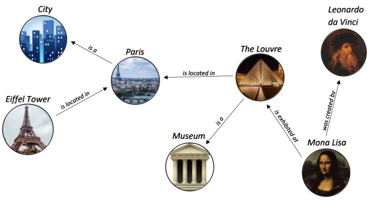
entities and r the relation between them. For example in the knowledge graph of
Figure 2.1, such a triple is the (“Eiffel Tower”, “is located in”, “Paris”) triple, where
“Eiffel Tower” and “Paris” are the entities and “is located in” is the relation between
4Figure 2.1: Example of a knowledge graph.
them or the (“Mona Lisa”, “was created by”, “Leonardo da Vinci”) triple, where “Mona
Lisa” and “Leonardo da Vinci” are the entities and “was created by” is the relation
between them.
Knowledge graphs are useful, because they combine characteristics of:
• Database, because the data can be explored via structured queries,
• Graph, because they can be analyzed as any other network data structure,
• Knowledge base, because they can be used to interpret the data and infer new
facts.
Knowledge graphs are used in many tasks in recent years, including question
answering, recommendation and information retrieval. They are associated with, and
used by search engines such as Google, Bing, and Yahoo; knowledge-engines and
question-answering services such as WolframAlpha, Apple’s Siri, and Amazon Alexa;
and social networks such as LinkedIn and Facebook.
Some of the biggest knowledge graphs are these of Microsoft (KG for the Bing
search engine, LinkedIn data and Academics), ebay (KG that gives relationships
within users and products, provided on the website), Google (KG for the categoriza-
tion function across Google’s devices and for the Google search engine) and Facebook
(KG for making connections among people, events, ideas and news). There are also
free and open knowledge graphs, like the Wikidata [11] (KG for Wikipedia and other
1
Wikimedia sister projects) or the Freebase [12] (KG that aims to create a global
1
The Freebase was officially closed on May 2, 2016 and the data was transferred to Wikidata
5resource that allow people (and machines) to access common information more ef-
fectively.).
2.2 Knowledge Graph Embeddings
The large volume of data, usually makes the traditional graph structure of the knowl-
edge graphs hard to manipulate. For this reason, the knowledge graph embeddings
are used instead.
KG embeddings encode entities and relations of a KG into vectors in some low
dimensional space, while preserving the information of the KG, see Figure 2.2.
These vectors (embeddings) can be used for a wide range of tasks such as clas-
sification, clustering, link prediction, and visualization. They make it easier to do
machine learning on large inputs and also vector operations are simpler and faster
than comparable operations on graphs. This make’s them also a useful tool for social
network analysis.
6Figure 2.2: Example of KG embeddings representation in the 2-dimensional vector
space.
2.3 Knowledge Graph Embedding Models
KG embeddings can be generated using a KG embedding model. A variety of KG
embedding models have been proposed to embed both entities and relations in knowl-
edge graphs into a low-dimensional vector space.
In general, if T is a set of triples, then a KG embedding model define a score
function f (e1 , r, e2 ) for each triple (e1 , r, e2 ) ∈ T . The score function f (e1 , r, e2 ) returns
a higher score, if the triple (e1 , r, e2 ) is true, than vice versa. Some KG embedding
models use a margin-based loss as the training objective to learn embeddings of the
entities and relations, while some others cast the training objective as a classification
task. The embeddings of the entities and relations can be learned by minimizing the
regularized logistic loss. The main difference among various KG embeddings models
is the score function they use.
Two widely known KG embedding models, which we also use in our experiments,
are the TransE [3] and the TransH [4] models. They both use a margin-based loss
L, based on the score function of each model, as the training objective to learn the
embeddings:
∑ ∑
L= [γ + f (e1 , r, e2 ) − f (e1 , r, e2 )′ ], (2.1)
(e1 ,r,e2 )∈T (e1 ,r,e2 )′ ∈T ′
where γ > 0 is a margin hyperparameter and T ′ denotes the set of non-existing triples,
which is constructed by corrupting entities and relations in the existing triples.
72.3.1 The TransE model
TransE [3] is the most representative translational distance model. The model rep-
resents the entities and the relations of the KG as translation vectors in the same
embedding space. Specifically, every entity such “Paris” or “City” and every rela-
tion such “is a” is represented as a d-dimensional vector, which includes the in-
formation of this entity or relation in the graph, and is now used instead of the
entity or the relation. Given a triple (e1 , r, e2 ), let e⃗1 , e⃗2 be the embeddings of en-
tities e1 and e2 , respectively, and ⃗r the embedding of the relation r. The idea in
TransE is that e⃗1 + ⃗r should be near to e⃗2 , if (e1 , r, e2 ) holds and e⃗1 + ⃗r should be
far away from e⃗2 , otherwise. Figure 6.1a gives an intuition, that is if, for exam-
ple, (‘‘M ona Lisa”, ‘‘was created by”, ‘‘Leonardo da V inci”) triple holds, then using
Transe model, ‘‘M ona ⃗ Lisa”+‘‘was created
⃗ by” should be near to ‘‘Leonardo⃗ da V inci”.
Specifically, the score function of the TransE model is:
f (e1 , r, e2 ) = −||e⃗1 + ⃗r − e⃗2 ||1/2 (2.2)
and the score is high if (e1 , r, e2 ) holds, while it is low otherwise.
2.3.2 The TransH model
TransH [4] is an also widely used KG embedding model. The difference of TransE
is that it introduces relation-specific hyperplanes. Specifically, in TransH the rep-
resentation of the entity is directly related to the relation to which it is associ-
ated. Given a triple (e1 , r, e2 ), the entity representations e⃗1 and e⃗2 are first projected
onto the r-specific hyperplane. Specifically, it is not used the d-dimensional em-
beddings of the entity “Paris”, for example, but the projection of it on the hyper-
plane based on the d-dimensional embedding of the relation we are interested in,
like the “is a” relation. The projections of the entities are then assumed to be con-
nected by ⃗r on the hyperplane with low error if (e1 , r, e2 ) holds, i.e., e⃗1⊥ + ⃗r ≈ e⃗2⊥ .
e⃗1⊥ and e⃗2⊥ are the projection embeddings of entities e1 and e2 on the relation-
specific hyperplane and ⃗r is the embedding of a relation r. In Figure 6.1b, for
example, if (‘‘M ona Lisa”, ‘‘was created by”, ‘‘Leonardo da V inci”) triple holds,
then using the TransH model, ‘‘M ona⃗ Lisa⊥ ” + ‘‘was created
⃗ by” should be near to
‘‘Leonardo⃗da V inci⊥ ”. So, the score function of the TransH model:
f (e1 , r, e2 ) = −||e⃗1⊥ + ⃗r − e⃗2⊥ ||2 , (2.3)
8(a) TransE (b) TransH
Figure 2.3: If (‘‘M ona Lisa”, ‘‘was created by”, ‘‘Leonardo da V inci”) triple holds,
then using Transe model ‘‘M ona ⃗ Lisa” + ‘‘was created
⃗ by” should be near to
‘‘Leonardo⃗ da V inci” and using TransH model, ‘‘M ona⃗ Lisa⊥ ” + ‘‘was created
⃗ by”
should be near to ‘‘Leonardo⃗da V inci⊥ ”.
is high if (e1 , r, e2 ) holds, while it is low otherwise.
2.3.3 Comparison of the two models
TransE is simple and efficient model, but it has flaws in dealing with 1-to-N, N-
to-1, and N-to-N relations [2]. For example, if “Leonardo da Vinci has occupation
painter” and also “Leonardo da Vinci has occupation engineer”; for 1-to-2 relation,
then Leonardo⃗ da V inci + has occupation
⃗ ⃗
must be close to painter, but it must also be
⃗
close to engineer. This means that for has occupation relation, engineer and painter
are similar, but this is not true. The problem gets worse as the tail entities increase.
To overcome the disadvantages of TransE, TransH introduces relation-specific hy-
perplanes. Specifically, it enables an entity to have distributed representations when
involved in different relations.
2.4 Notations
From here on we will use e1 for the head entity of a triple, e2 for the tail entity and
r for the relation. We will also use ⃗e for the TransE embedding of an entity e and e⃗⊥
for the TransH embedding of an entity e.
9CHAPTER 3
BIAS IN THE DATASET
3.1 Metrics for measuring bias in the dataset
In this chapter we present some metrics for measuring bias in the dataset. We expect
that the dataset contains bias, because the data come from real life, where bias and
inequality are a constant problem. To find out if the bias exists and to quantify this
bias, we consider two approaches.
3.1 Metrics for measuring bias in the dataset
Let s be a sensitive attribute (e.g. gender) and a, b two sensitive values (e.g. male,
f emale). Let’s also consider, that we want to discover if there is bias in occupations,
because of the sensitive attribute s. To do this, we consider two approaches: we (a)
look at both the expected number and the actual number of a-value entities (e.g male
entities) and b-value entities (e.g. f emale entities) (equal opportunity approach),
and (b) look only at the actual number of a-value entities and b-value entities (equal
number approach).
3.1.1 Equal opportunity approach
Definition 3.1. We want the probability that an individual has a specific occupation
o to be the same for entities with a value and entities with b value, or, in other words,
10we ask that the probability that an individual has occupation o does not depend on
the sensitive attribute s of the person.
P (O = o|S = a) = P (O = o|S = b) (3.1)
3.1.2 Equal number approach
Definition 3.2. Given an occupation o, we ask that it is equally probable that the
individual who has this occupation has value a or b.
P (S = a|O = o) = P (S = b|O = o) (3.2)
3.1.3 Measuring bias in data with the two approaches
From the Bayes rule
P (O = o|S = a)P (S = a)
P (S = a|O = o) = (3.3)
P (O = o)
P (O = o|S = b)P (S = b)
P (S = b|O = o) = (3.4)
P (O = o)
The two definitions are equivalent if the numbers of entities with a value and
entities with b value in the population are equal.
To estimate them, let,
Ao Bo
P (S = a|O = o) = , P (S = b|O = o) = ,
Ao + Bo Ao + Bo
A B Ao + Bo
P (S = a) = , P (S = b) = , P (O = o) = ,
A+B A+B A+B
Ao Bo
P (O = o|S = a) = , P (O = o|S = b) = ,
A B
where A, B are the individuals have the values a, b, respectively. Also, Ao , Bo are the
a-value individuals and the b-value individuals have an occupation o, respectively.
So, we can measure how much biased an occupation is, by taking the difference
or the ratio.
Definition 3.3 (difference for equal opportunity).
Ao Bo
ϕo = P (O = o|S = a) − P (O = o|S = b) = − (3.5)
A B
11Definition 3.4 (ratio for equal opportunity).
Ao
P (O = o|S = a) A Ao B
ϕo = = Bo
= (3.6)
P (O = o|S = b) B
Bo A
Definition 3.5 (difference for equal number).
Ao − Bo
ϕo = P (S = a|O = o) − P (S = b|O = o) = (3.7)
Ao + Bo
Definition 3.6 (ratio for equal number).
P (S = a|O = o) Ao
ϕo = = (3.8)
P (S = b|O = o) Bo
In both difference definitions, ϕo ∈ [−1, 1]. We call occupations for which ϕo > 0
“a biased”, occupations for which ϕo < 0 “b biased” and occupations for which
ϕo = 0 “neutral”. Also, in both ratio definitions, ϕo ∈ [0, ∞]. We call occupations for
which ϕo > 1 “a biased”, occupations for which ϕo < 1 “b biased” and occupations
for which ϕo = 1 “neutral”. To have the same range, [−1, 1], in difference and ratio
definitions, we can make the transformation:
• if ϕo < 1, then ϕ′o = ϕo − 1,
• if ϕo > 1, then ϕ′o = 1 − 1
ϕo
,
• if ϕo = 1, then ϕ′o = 1 − ϕo
In addition to occupations that have a zero score, we consider also neutrals those
occupations that belong to a range close to zero. Τhis range is defined by a constant t.
To set threshold t, we plot the distribution of neutral occupations for different values
of t and select the value of t for which there is a sharp increase in the number of
neutral occupations in the plot.
12CHAPTER 4
BIAS IN KNOWLEDGE GRAPH EMBEDDINGS
4.1 Methods for measuring bias in knowledge graph embeddings
4.2 Clustering fairness using knowledge graph embeddings
In this chapter we present some methods to study first, if the bias information is
transferred from the data to the KG embeddings and then to detect if there is am-
plification of bias using the embeddings. We also present an approach to recognize
if clusters produced by the KG embeddings are fair or the bias affects the clustering
procedure.
4.1 Methods for measuring bias in knowledge graph embeddings
We define here a method based on projections on a bias direction and an analogy
puzzle to detect if KG embeddings contain bias. We also present a prediction method
to examine bias augmentation using the embeddings.
4.1.1 Projection method
The idea in this method is that there is a bias direction, which includes the information
of the bias. For example if gender is the sensitive attribute, then we consider that exists
a gender bias direction with the gender information. We explain below how we choose
this direction.
13Given the bias direction, the projection of an occupation embedding on this direc-
tion gives the bias information, which is included in the embedding. Moreover, the
norm of the projection shows how much bias information the embedding contains. So
the greater the norm of this projection is, the more bias information the embedding
includes.
Let ⃗o be the embedding of an occupation o, and d⃗ the bias direction. Then, the
quantity of bias, which contains the occupation embedding, is:
||πd⃗ ⃗o||, (4.1)
where πd⃗⃗o = ⃗o · d⃗ is the projection of ⃗o onto d.
⃗
Bias direction
To define the best gender bias direction in [6] using word embeddings, they use
the embeddings of pairs of words showing gender bias, like (male, female), (father,
mother), (brother, sister), etc. Then, they use SVD to the vector resulting from the
differences of the embeddings of the bias pairs. So the top-singular vector is the bias
direction for the word embeddings. We use this idea, but knowledge graph embed-
dings are different from word embeddings. The gender information, for example, in
word embeddings, learned from the sentences in the text. On the other hand in KG
embeddings there are triples and specific entities that express the bias. So if we care
about the gender bias, as before, the entities male and female contain all the gender
bias information, because all the males are connected with the male entity with triples
(“male entity”, “has gender”, “male”) and all the females are connected with the fe-
male entity with triples (“female entity”, “has gender”, “female”). So we conclude
that the best choice for the bias direction is the subtraction of the male, female entity
⃗
embeddings (f emale ⃗
− male). We do not need to take SVD, because we have only one
pair of entities, that clearly expresses the bias. The only different for the embeddings
produced by the TransH model is that they are projections on the relation-specific
hyperplane, “has gender” in our case. So the direction, taking into account this in-
⃗ ⊥ − male
formation, will be (f emale ⃗ ⊥ ). In general, for a sensitive attribute s and two
sensitive values a and b the bias direction using TransE KG embeddings is:
d⃗ = ⃗b − ⃗a (4.2)
14and the bias direction using TransH KG embeddings is:
d⃗ = b⃗⊥ − a⃗⊥ (4.3)
Comparison of our embedding bias metric with an other existing metric
The only other metric for measuring bias in KG embeddings is this in [1]. Using
this metric, if gender is the sensitive attribute and male, f emale the two sensitive
values, then the entity embeddings are first transformed to be “more male” according
to the model’s own encoding of masculinity. Then using all the individuals in the
dataset, they analyse whether, making an entity more male increases or decreases the
likelihood that they have an occupation, according to the model’s score function.
So the first difference with our metric is that they use a transformation of the
individuals’ embeddings to measure the bias in occupations. On the other hand we
use only the embeddings of the occupations and a bias direction to quantify the bias
information, that is more simple but also effective. Another difference is that they
use the whole number of individuals in the dataset to separate the occupations into
male and female occupations. This is particularly time consuming especially in large
datasets, where there are millions of individuals and occupations. Instead of this we
suggest to use the similarity with the sensitive values (male, female) to separate the
occupations. This is based on the idea that the information which creates the bias is
this of the sensitive values that is included in the embedding. For example, doctor
is considered as male occupation because the “male information” is included in the
embedding of doctor. Also all the embeddings of the male individuals contain the male
information. So we can use instead of the male individuals, which can be millions,
the male entity and respectively, instead of the female individuals, the female entity.
The last difference concerns the correlation of bias with popularity, and is analyzed
in section 6 with experimental evaluation. Our metric, in contrast with the metric in
[1], includes the popularity information in bias score and this is important because,
as we show later, popularity affects bias.
4.1.2 Analogy puzzle method
Inspired from [6] and word embeddings, we use an analogy puzzle to detect if KG
embeddings contain bias. To do this we try to find pairs of occupations, which are
close to the parallel to a seed direction. The seed direction in our case is the bias
15You can also read