Rear end crash simulation using Human Body Models
←
→
Page content transcription
If your browser does not render page correctly, please read the page content below
Rear end crash simulation using Human
               Body Models
An investigation of the design of seat structure using a 50th percentile female
                             Human Body Model

                                Jacob Fagerström

                Mechanical Engineering, master's level (120 credits)
                                      2020

                               Luleå University of Technology
                      Department of Engineering Sciences and Mathematics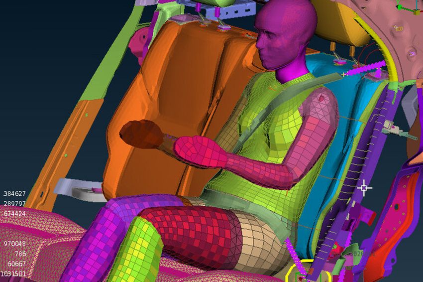
Abstract
In this master thesis it have been investigated how the stiffness of a seat affect the risk of neck injuries,
e.g whiplash associated disorders, in a rear end low velocity car collision using a female human body
model, HBM, and if dividing the seat into several sections with different stiffnesses. The project is
performed in collaboration with CEVT, China Euro Vehicle Technology, a innovation center of the
Geely Holding Group. The HBM used is the VIVA open source HBM developed by Chalmers University
of Technology together with Volvo Cars, The Swedish National Road and Transport ResearchInstitute
(VTI) and Folksams forskningsstiftelse. Two different seats were investigated, a generic seat and the
seat of the existing Lynk&Co 01. The stiffness of the seat had a significant impact on the risk of neck
injuries, but does not seem to be a good idea to divide the seat into several sections since the height
of the individual in the seat influence what stiffness is optimal for each section. It was also discovered
that the relative distance between the head and the headrest at the moment of impact has a great
affect on the risk of neck injuries.

                                                      i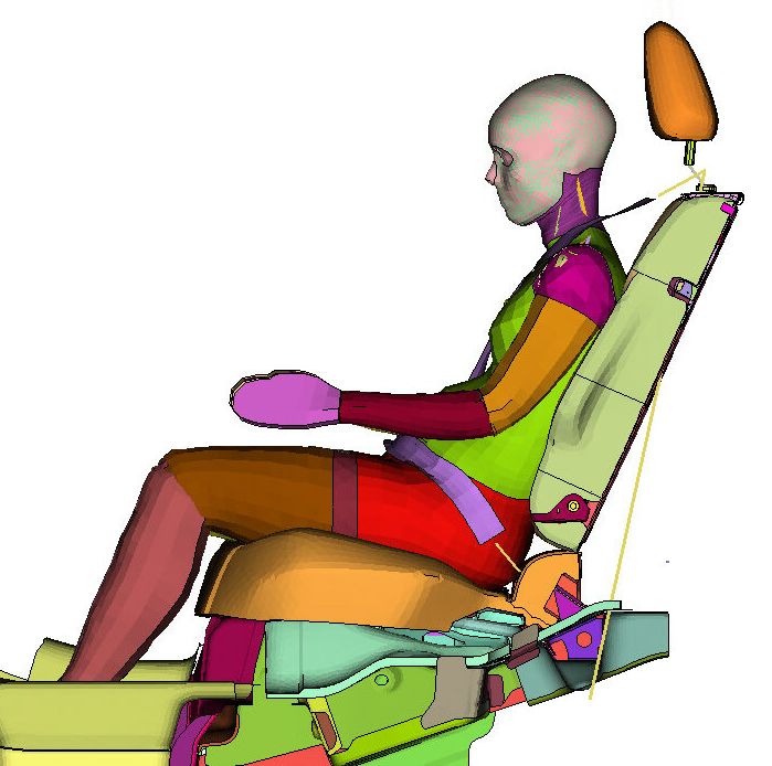
Acknowledgements
I would like to thank CEVT for hosting, helping and supporting me during my work. Halfway through
the work COVID-19 hit the world and everyone were ordered to work from home, it was an unforseen
change that made things slightly more difficult but CEVT handled the situation admirable. A special
thanks to my supervisors at CEVT Dag Thuvesen, Robert Karlsson, Pooja Umeshkumar and Robert
Persson for their help and support, thank you for all the input and advice you gave me, it was a great
comfort to know that I had you to turn to if I would need help. I have greatly enjoyed working with
you, and my supervisor at LTU Paul Åkerström for his help and support, during the entire project it
never took you more than a day to answer any questions I had or give me feedback on my work. I
greatly appreciate that. This would not have been possible without all of you

                                                                                 Jacob Fagerström
                                                                                        June 2020

                                                  ii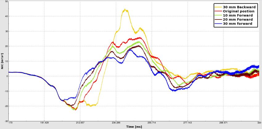
Contents
1 Introduction                                                                                                                                                                  1
  1.1 Background . . . . . . . . . . . . . . . . . . . . . . . . . . . . . . . . . . . . . . . . . . .                                                                          1
  1.2 Problem formulation . . . . . . . . . . . . . . . . . . . . . . . . . . . . . . . . . . . . . .                                                                           1
  1.3 Software . . . . . . . . . . . . . . . . . . . . . . . . . . . . . . . . . . . . . . . . . . . . .                                                                        2

2 Theory                                                                                                                                                                        5
  2.1 Implicit and explicit solvers .     .   .   .   .   .   .   .     .   .   .   .   .   .   .   .   .   .   .   .   .   .   .   .   .   .   .   .   .   .   .   .   .   .   5
  2.2 Whiplash associated disorder        .   .   .   .   .   .   .     .   .   .   .   .   .   .   .   .   .   .   .   .   .   .   .   .   .   .   .   .   .   .   .   .   .   5
  2.3 Injury criteria . . . . . . . . .   .   .   .   .   .   .   .     .   .   .   .   .   .   .   .   .   .   .   .   .   .   .   .   .   .   .   .   .   .   .   .   .   .   6
  2.4 Response surface method . .         .   .   .   .   .   .   .     .   .   .   .   .   .   .   .   .   .   .   .   .   .   .   .   .   .   .   .   .   .   .   .   .   .   7

3 Method                                                                                                                                                                       8
  3.1 Positioning of the Human Body Model . .                           .   .   .   .   .   .   .   .   .   .   .   .   .   .   .   .   .   .   .   .   .   .   .   .   .   . 8
  3.2 Setup generic seat and HBM . . . . . . .                          .   .   .   .   .   .   .   .   .   .   .   .   .   .   .   .   .   .   .   .   .   .   .   .   .   . 9
  3.3 Generic seat parameter investigation . . .                        .   .   .   .   .   .   .   .   .   .   .   .   .   .   .   .   .   .   .   .   .   .   .   .   .   . 12
  3.4 Setup Lynk&Co 01 seat and HBM . . . .                             .   .   .   .   .   .   .   .   .   .   .   .   .   .   .   .   .   .   .   .   .   .   .   .   .   . 12
  3.5 Lynk&Co 01 seat parameter investigation                           .   .   .   .   .   .   .   .   .   .   .   .   .   .   .   .   .   .   .   .   .   .   .   .   .   . 12

4 Result                                                                                                                                                                        17

5 Discussion                                                                                                                                                                    26
  5.1 Injury criteria . . . . . . . . . . . . . . . . . . . . . . . . . . . . . . . . . . . . . . . . . .                                                                       26
  5.2 Positioning of the model . . . . . . . . . . . . . . . . . . . . . . . . . . . . . . . . . . . .                                                                          26
  5.3 Seat parameter investigation . . . . . . . . . . . . . . . . . . . . . . . . . . . . . . . . .                                                                            26

6 Conclusion                                                                                                                                                                    30

A Appendix A                                                                                             A1
  A.1 Generic seat . . . . . . . . . . . . . . . . . . . . . . . . . . . . . . . . . . . . . . . . . . . A1
  A.2 Original Lynk&Co 01 setup . . . . . . . . . . . . . . . . . . . . . . . . . . . . . . . . . . A13
  A.3 Lynk&Co 01 setup with moved headrest . . . . . . . . . . . . . . . . . . . . . . . . . . . A26

                                                                  iii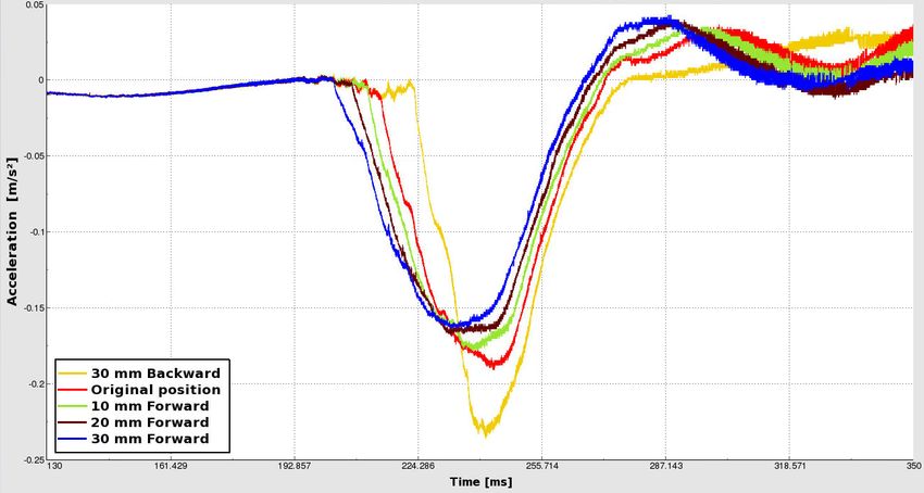
1     Introduction
In this master thesis the VIVA open source Human Body Model, HBM, developed by Chalmers Uni-
versity of Technology together with Volvo Cars, The Swedish National Road and Transport Research
Institute (VTI) and Folksams forskningsstiftelse will be used to investigate how different parameters
affect the safety of a 50th percentile female riding in the back seat during a low velocity rear impact,
around 16 km/h, [1][2]. The thesis project is performed in collaboration with CEVT, China Euro
Vehicle Technology AB. CEVT is a part of the Geely Holding Group and is an innovation center,
developing automotive technology that will meet the demands of tomorrow’s global market. With
their advanced virtual engineering, software development and modular development they are able to
deliver world-class technology to all Geely Group brands [3][4].

1.1     Background
There is a constant ongoing effort in the automotive industry to increase the safety for everyone inside
and outside of a car. One of the steps to improving safety for individuals inside a car is to perform crash
tests. These test provides concrete information of how well suited a car is for different crash scenarios.
However, there are some problems with these tests. It is rather expensive to build a prototype and
crash it, it is time consuming, both for building and for analysing the result, especially if it is a new
model that is not yet in production. As computers have become more and more powerful much of the
testing that was done with prototypes and models are now simulated on a computer instead. It is both
cheaper and faster than performing physical tests. When it comes to car crash simulations the use of
crash test dummies plays a major role. The first crash test dummies were developed during the 1950s
and are continuously developed further. There also exists finite element crash dummy models to be
used in crash simulations [5]. During the last 40 years human body models have been developed and
improved and there is a belief that they will give an even more realistic result from crash simulation
and aid in the battle against injuries, such as whiplash associated disorders, WADs, in car crashes[6].
In Sweden, WADs are responsible for about 50 % of all personal injuries that lead to long term health
loss from motor accidents in Sweden and half of these injuries are a result of rear impacts [7].
When it comes to WADs, females are at a greater risk than men, as shown in Figure 1, but until recently
there were a shortage of available female test models, Figure 2, so despite being over represented in
injury statistic females were underrepresented when it came to safety testing. This is something that
is being addressed in the industry, partly by the creation of the EvaRID FE model, the BioRID50F
dummy and the VIVA OpenHBM F50 FE model. The main differences between a HBM and a FE
model of a crash test dummy is that a HBM can be used in every sort of crash while different crash
test dummies is used for different sort of impact directions, since a dummy is designed to withstand a
crash test to be able to use them again, a HBM might detect something that a dummy model might
miss due to its design [1][8].

1.2     Problem formulation
Investigate how the VIVA HBM developed by Chalmers University of Technology [1] can be imple-
mented in a rear end car crash simulation and investigate how design parameters of the seat will affect
the injuries. First step is to investigate different ways to position the HBM, then a crash simulation for
a generic seat will be conducted and different parameter of the seat will be investigated using design of
experiments, DOE. Then the same simulations will be conducted but with a Lynk&Co 01 seat instead
to see if the result will follow the same behaviour. So in summary:
    1. Positioning the model
    2. Investigate the influence of the stiffness of the backrest on generic seat
    3. Investigate the influence of the stiffness of the backrest in a Lynk&Co 01 seat

                                                     1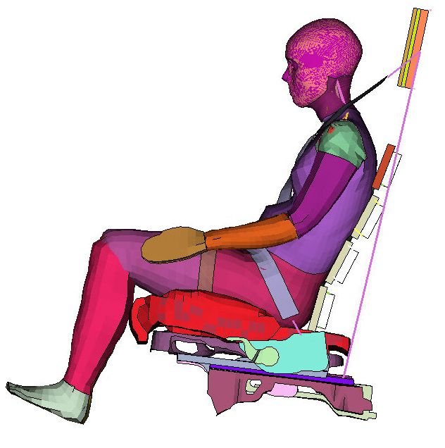
Figure 1: A comparison of the relative risk of whiplash injuries from several studies, it is clear that in all studies the
females are at greater risk than men. Accessed from [8]

Figure 2: A visualisation of the existing crash test dummies used for front and rear end impact testing in 2012 and
the stature distribution of British male, dark grey, and British female, light grey. It is clear that a large portion of the
population is unrepresented. Accessed from [8].

1.3     Software
During this master thesis mainly four different software have been used. Two from BETA CAE Sys-
tems, the pre-processor ANSA and the post-processor BETA, and two from Livermore Software Tech-
nology, the finite element program LS-DYNA and the optimization program LS-OPT. The following
descriptions of the programs are quotes from the companies descriptions of their own products.

                                                             2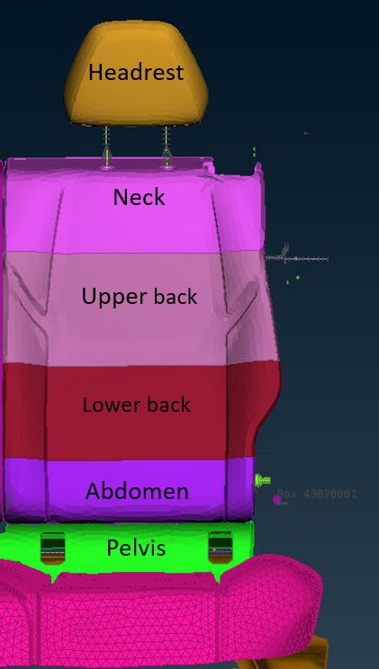
ANSA
   ”ANSA is an advanced multidisciplinary CAE pre-processing tool that provides all the
   necessary functionality for full-model build up, from CAD data to ready-to-run solver
   input file, in a single integrated environment. ANSA is the users’ preference due to its
   wide range of features and tools that meet their needs. The list of productive and versatile
   features is long and the alternative tasks and processes to be completed using them are
   countless.” [9]

META
   ”META is a thriving multi-purpose post-processor meeting diverging needs from various
   CAE disciplines. It owes its success to its impressive performance, innovative features and
   capabilities of interaction between animations, plots, videos, reports and other objects.”
   [10]

LS-DYNA
   ”LS-DYNA is a general-purpose finite element program capable of simulating complex real
   world problems. It is used by the automobile, aerospace, construction, military, manufac-
   turing, and bioengineering industries. LS-DYNA is optimized for shared and distributed
   memory Unix, Linux, and Windows based, platforms, and it is fully QA’d by LSTC. The
   code’s origins lie in highly nonlinear, transient dynamic finite element analysis using explicit
   time integration.”
   ”LS-DYNA’s potential applications are numerous and can be tailored to many fields. In a
   given simulation, any of LS-DYNA’s many features can be combined to model a wide range
   of physical events. An example of a simulation, which involves a unique combination of
   features, is the NASA JPL Mars Pathfinder landing simulation which simulated the space
   probe’s use of airbags to aid in its landing. LS-DYNA is one of the most flexible finite
   element analysis software packages available.
   LS-DYNA consists of a single executable file and is entirely command line driven. Therefore
   all that is required to run LS-DYNA is a command shell, the executable, an input file, and
   enough free disk space to run the calculation. All input files are in simple ASCII format
   and thus can be prepared using any text editor. Input files can also be prepared with the
   instant aid of a graphical preprocessor.
   There are many third party software products available for preprocessing LS-DYNA input
   files. LSTC also develops its own preprocessor, LS-PrePost, which is freely distributed
   and runs without a license. Licensees of LS-DYNA automatically have access to all of the
   program’s capabilities, from simple linear static mechanical analysis up to advanced thermal
   and flow solving methods. Furthermore, they have full use of LS-OPT, a standalone design
   optimization and probabilistic analysis package with an interface to LS-DYNA.”[11]

LS-OPT
   ”LS-OPT is a standalone Design Optimization and Probabilistic Analysis package with an
   interface to LS-DYNA.
   In the ”conventional design” approach, a design is improved by evaluating its ”response”
   and making design changes based on experience or intuition. This approach does not
   always lead to the desired result, that of a ‘best’ design, since the design objectives are
   often in conflict. It is therefore not always clear how to change the design to achieve the
   best compromise of these objectives. A systematic approach can be obtained by using

                                                  3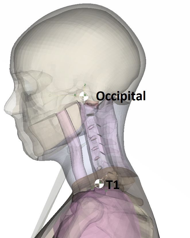
an inverse process of first specifying the criteria and then computing the ‘best’ design
according to a formulation. The improvement procedure that incorporates design criteria
into a mathematical framework is referred to as Design Optimization This procedure is
often iterative in nature and therefore requires multiple simulations.
No two products of the same design will be identical in performance, nor will a product
perform exactly as designed or analyzed. A design is typically subjected to Structural
variation and Environmental variation input variations that cause a variation in its response
that may lead to undesirable behavior or failure. In this case a Probabilistic Analysis, using
multiple simulations, is required to assess the effect of the input variation on the response
variation and to determine the probability of failure.
To run and control multiple analyses simultaneously, LS-OPT provides a simulation envi-
ronment that allows distribution of simulation jobs across multiple processors or networked
computers. Each job running in parallel consists of the simulation, data extraction and disk
cleanup. Measurements of time remaining or performance criteria such as velocity or energy
are used to measure job progress for LS-DYNA’s explicit dynamic analysis calculations.”
[12]

                                              4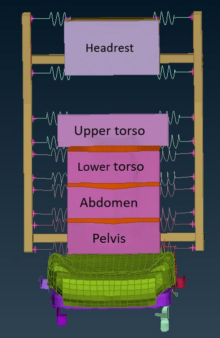
2     Theory
This section covers the fundamental theory that has been used.

2.1    Implicit and explicit solvers
When it comes to the Finite Element Method there are two different solving strategies. Implicit and
explicit solvers, also known as time independent and time dependent solvers. Consider the following
example:
Find x = x(t) such that                         (
                                                    ẋ = f (x, t)
                                                                                                             (1)
                                                    x(t0 ) = x0

Discretization of the time, t, so that t ∈ [t0 , t0 + ∆t, t0 + 2∆t, ..., t0 + n∆t] gives the possibility to solve
the ODE using either the Forward Euler’s method,

                                          xn+1 = xn + ∆tf (xn , tn ),                                        (2)

or the Backward Euler’s method,

                                       xn+1 = xn + ∆tf (xn+1 , tn+1 ),                                       (3)

among others [13][14]. The Forward Euler’s method is an explicit solver. Everything is known and the
next position of the equation can be calculated. However, this method is conditionally stable, i.e the
time step ∆t must be sufficiently small to give a stable solution. This is the case for every explicit
solver [13]. To ensure a sufficiently small timestep the Courant-Friedrichs-Lewy condition, CFL, must
be met. CFL states that the timestep must be equal to, or smaller than the time it would take a wave
to move through a discrete element. For 3D continuum this time step can be calculated using the
following equations:                          s
                                                    E(1 − ν)
                                         c=                                                        (4)
                                                (1 + ν)(1 − 2ν)ρ
                                                       l
                                               ∆t ≤ .                                               (5)
                                                      c
where c is the propagation speed of the wave and l is the element length [13][14][15][16]. The Backward
Euler’s method do not have to fulfill the CFL since it uses an iterative root-finding method, such as
the Newton-Raphson method or regula falsi. This iterative process can be quite calculation heavy
and time consuming, but the fact the number of time steps can be lowered can make the implicit
method faster than the explicit, but high frequency information from the transient solution may be
lost [14][17][18].

2.2    Whiplash associated disorder
Whiplash is a collective name used for injuries to the neck often caused by sudden stop or movement.
The injuries are especially associated with motor accidents. It was during the 1980s that whiplash
started to affect numerous people around the world. Much time, effort, and resources have been spent
on researching, and trying to prevent, whiplash associated disorders, but there are still no generally
accepted description, diagnose, or cause. The name whiplash comes from the fact that the injuries
occur due to a forceful and quick back and forth motion of the neck, similar to the cracking of a whip
[8][19].

                                                          5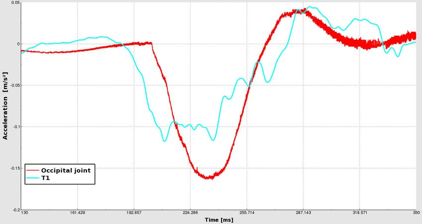
2.3     Injury criteria
To evaluate the risk of WAD injuries two different injury criterion’s have been used, the head injury
criterion and the neck injury criterion.

Head Injury criterion, HIC
The Head Injury Criteria, HIC, is an integration criteria that evaluates the risk of human brain injury
induced by impact, and is the factor that has the greatest influence on the survival rate. It is calculated
as                                                (        Z t2       2.5           )
                                                        1
                      HIC =           max                        a(t)dt     (t2 − t1 )                  (6)
                                t1 ,t2 ,t2 −t1 ≤∆    t2 − t1 t1

,where a is the resultant acceleration at the center of mass of the brain measured in the gravi-
tational constant g, t1 and t2 are arbitrary values chosen to maximise HIC, the duration of t2 − t1 is
limited to 15 ms or 36 ms. A value of 1000 is regarded as critical and exceeding this value indicates a
real threat of severe head injuries [8][20][21].

Neck Injury criterion, NIC
The Neck Injury Criterion, NIC, is calculated via
                                                                2
                                              N IC = 0.2arel + vrel                                              (7)
where the constant 0.2 has the unit m, arel is the relative horizontal acceleration between the occipital
joint and T1, and vrel is the relative horizontal velocity between the occipital joint and T1, Figure 3,
and calculated as                                    Z
                                             vrel = arel .                                            (8)

The critical value for NIC is somewhat debated. Kullgren et al.[22] stated that a NIC value of 15
m2 /s2 means an approximately 20 % risk of neck injuries lasting over one month. But Linder et al[23]
state that a NIC value of 16.7 m2 /s2 only corresponds to a 10 % risk of injuries lasting over one month
[8][24].

Figure 3: An illustration of the occiputal joint and T1. T1 located where the neck meets the torso, and the occipital
joint is located where the spine meets the head.

                                                         6
2.4 Response surface method
The response surface method is used to investigate the relationship between independent variables and
response variables. It is easiest to explain using an example, assume an unknown function f (x1 , x2 ),
if some values of f is known for x1 and x2 a response surface can be approximated using a fitting
method and a chosen order of the response surface. Figure 4. More known values obviously gives a
better fitting and an increase of independent variables demands an increase of data points to get a
good fitting. This method can be applied to highly non-linear responses and does not require any
analytical design sensitivities. [24][25][26].
Figure 4: A visualization of a response surface approximated from five response values, the function f (x1 , x2 ) has two
explanatory variables x1 and x2 . Accessed from [25].
73 Method
In this part the different methods that were investigated or used during the project are described. The
units used in the simulations are mm, ms, kN and kg.
3.1 Positioning of the Human Body Model
The positioning of the model is divided into two different steps. First step is to ensure the correct
body position for the HBM and the second step is to position at the right position in the crash model.
For the second step, the LS-DYNA keyword INCLUDE TRANSFORM and DEFINE TRANSFORMATION
were used [27].
To achieve the correct body position, two different approaches were investigated, the Prescribed
Displacement method and the Marionette Method. The idea of the Prescribed Displacement
method is to choose a number of nodes, that are a part of one or more rigid elements, and use the
LS-DYNA command BOUNDARY PRESCRIBED MOTION NODE to move these nodes into a desired
position. When using the BOUNDARY PRESCRIBED MOTION NODE command the user have the
option to choose to define the motion by velocity, acceleration, or displacement as a function of
time by selecting the corresponding flag when defining the keyword. In this project the displace-
ment flag was used and the displacement was described using a load curve with a ramp up, ramp
down and a settling phase to get a smooth motion. The ramping curve is illustrated in Figure 5 [14][27].
Figure 5: Curve with continues ramping for describing the displacement for nodal motion. From 0 to T is the displacement
phase, and from T to 2T is the settling phase [14].
The marionette method uses a cable between node pairs to move the model into a desired position. The
nodes that are chosen should be a part of a rigid element, or a fixed node in space. A cable is created
between the two nodes using ELEMENT BEAM ELFORM 6 together with MAT CABLE DISCRETE BEAM.
The beam has an initial tensile force, that is defined in the material card, and that force moves the
HBM. The E variable should be set to 0 to avoid added mass as the length of the cables approaches
zero. To assign the material to the element the keyword SECTION BEAM ELFORM 6 is used. To
help the model to settle after displacement dampers are used. The dampers are defined using in a
similar way as the cables but with the keywords ELEMENT DISCRETE, MAT DAMPER VISCOUS, and
SECTION DISCRETE. Each node pair needs a cable and a damper to achieve a smooth motion. To
avoid error termination it is important to assign mass to nodes that are fixed in space, this is done by
using the keywords SET NODE and ELEMENT MASS NODE SET [27][28].
8After consultation from Karl-Johan Larsson and I Puta Alit Putra at Chalmers University of
Technology it was decided to use the marionette method to position the dummy. The reasoning and
the pros and cons with the two methods can be found in section 5.
3.2 Setup generic seat and HBM
Once that HBM was correctly positioned together with the seat, a 3-point seatbelt was added using
ANSAs SeatBelt option [29]. The 1-D elements were assigned the material data according to Table 1
and the 2-D Shell elements the material data presented in table 2.
Table 1: A table of the data used on the keycard MAT SEATBELT for describing the material of 1-D seatbelt
elements. The load curve for loading and unloading can be seen in Figure 6, inputs not defined are set to their
default values.
Option Value
MPUL 5.E-5
LLICD See Figure 6
ULICD See Figure 6
LMIN 1
Table 2: A table of the data used on the keycard MAT ELASTIC for describing the material of 2-D shell
elements used for a seatbelt. Inputs not defined are set to their default values.
Option Value
RO 7.85E-6
E 210
PR 0.3
Figure 6: The load curve used as input for loading and unloading, force vs. engineering strain, for 1-D seatbelt elements.
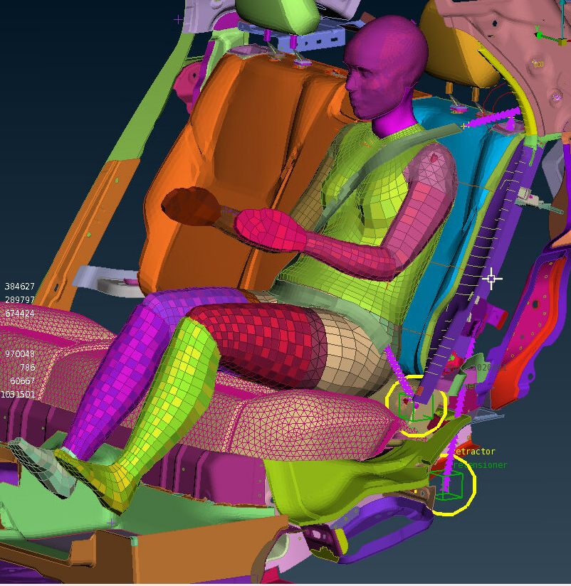
The seatbelt is equipped with two retractors and two pretensioners, as seen in Figure 7, the settings
for the pretensioners and the retractors can be found in table 3 and 4, the pretensioners are triggered
at the start of the simulations by a time sensor, ELEMENT SEATBELT SENSOR. Gravity is applied
9using the keyword LOAD BODY OPTION, with a load value of 0.00981. For the crash pulse the keyword
BOUNDARY PRESCRIBED MOTION RIGID ID was used with the acceleration flag activated and the load
curve shown in Figure 10. The motion has its birth set to 300 to give the HBM time to settle in the
seat and the pretensiors to finish their task.
Figure 7: The model and the seat with the seatbelt. Here the position of the two retractors and pretensioners can be
seen.
Table 3: A table of the data used on the keycard ELEMENT SEATBELT PRETENSIONER. Inputs not listed
are set to their default values.
Option Value
SBPRTY 7
TIME 0
PTLCID See Figure 8
10Table 4: A table of the data used on the keycard ELEMENT SEATBELT RETRACTOR. Inputs not listed are
set to their default values.
Option Value
TDEL 0
PULL 0.5
LLCID See Figure 9
ULCID See Figure 9
LFED 4
Figure 8: The load curve used by the pretensioners. It has the constant value of 0.05
Figure 9: The load curve used by the retractors for loading and unloading.
11Figure 10: Load curve describing the acceleration versus time for the crash pulse. Since the seat is positioned in such
a way that forward for the seat is in the negative x-direction the acceleration is negative. The final velocity after the
acceleration is close to 15.7 km/h
3.3 Generic seat parameter investigation
In Figure 12a it can be observed that the backrest consist of four panels, plus one panel for the
headrest. These panels are attached to the rigid seat frame with spring elements, the stiffness of each
panel is controlled by changing the stiffness coefficient for the springs responsible for each panel, so
in total five parameters are changed. This is performed in LS-OPT and the stiffness coefficients are
defined to be continuous with a value between 5 and 20 kN/m. The response surface is calculated
using a the polynomial method of the quadratic order with a total of 50 simulation points, default
number of simulation points for five parameters is set to 32 in LS-OPT, selected by LS-OPT using the
D-Optimal point selection scheme, which aims to minimize the determinant of the moment matrix and
is the recommended point selection scheme for polynomial response surface by LS-OPT [24].
3.4 Setup Lynk&Co 01 seat and HBM
The setup for the Lynk&Co 01 seat was made as similar to the generic seat as possible to favour a fair
comparison between the two seats. A 3-point seatbelt was added using ANSAs SeatBelt option[29],
just as it had with the generic seat, the 1-D elements had the material data according to table 1 and
the 2-D Shell elements had the material data presented in table 2.
The seatbelt is equipped with two retractors and two pretensioners, as seen in Figure 11, the settings
for the pretensioners and the retractors can be found in table 3 and 4, the pretensioners are triggered
at the start of the simulations by a time sensor, ELEMENT SEATBELT SENSOR. Gravity is applied
using the keyword LOAD BODY OPTION, with a load value of 0.00981. For the crash pulse the keyword
BOUNDARY PRESCRIBED MOTION RIGID ID was used with the acceleration flag activated and the load
curve shown in Figure 10. The motion has its birth set to 160 to give the HBM time to settle in the
seat and the pretensiors to finish their task.
3.5 Lynk&Co 01 seat parameter investigation
The backrest of the Lynk&Co 01 seat is divided into five sections, plus the headrest, as can be seen in
Figure 12b. The material used is MAT LOW DENSITY FOAM and the stiffness of the material is defined
using the stress-strain curve shown in Figure 13 for the backrest, and the stress-strain curve shown in
Figure 14 for the headrest. To change the stiffness, a scale factor ranging from 0.5 to 5 with a initial
value of 1 for the backrest, and a scale factor ranging from 0.002 to 0.02 with a initial value of 0.0045
12Figure 11: A visualisation of the setup of the HBM model and the seat with the seatbelt. Some parts of the car have
been hidden to better illustrate the setup.
13for the headrest was used on the Y values of the two graphs. In total six parameters. The response
surface is calculated using a the polynomial method of the quadratic order with a total of 70 simulation
points, default number of simulation points for five parameters is set to 48 in LS-OPT, selected by
LS-OPT using the D-Optimal point selection scheme, which aims to minimize the determinant of the
moment matrix and is the recommended point selection scheme for polynomial response surface by
LS-OPT [24].
The result was not as conclusive as desired, therefore another setup with a total of 70 simulation points
for the Lynk&Co 01 seat was performed but with slight alterations. The difference compared to the
previous setup was that the range of the scale factor for the headrest was increased to be from between
0.002 and 0.02 to range between 0.002 and 0.04, and the headrest was moved 30 mm towards the rear
of the car, as can be seen in Figure 16, to better match the generic seat, Figure 15.
Once again the result for the different sections was not as conclusive as desired, but it was noticed
that the range for the NIC and the HIC values had about the same span in both simulations but the
median was noticeably higher. To investigate how the position of the headrest influenced the response
values three more simulations was performed were the headrest was moved 10, 20, and 30 mm towards
the front of the car from its original position, while the scale factors for the different sections of the
seat was kept at their initial values. Together with the two previous positions of the headrest a total
of five positions have then been investigated.
(a) Generic seat (b) Lynk&Co 01 seat
Figure 12: The Lynk&Co 01 seat and the generic seat and the name used for the different sections of each seat. The
Lynk&Co 01 seats backrest is divided into five sections plus the headrest, and the generic seat is divided into four
sections plus the headrest.
14Figure 13: The stress-strain curve used for the materials in the five sections in the backrest of the Lynk&Co 01 seat.
This is the initial curve where the scale factor applied to the Y-axis is set to 1.
Figure 14: The stress-strain curve used for the materials in the headrest of the Lynk&Co 01 seat. This is the initial
curve where the scale factor applied to the Y-axis is set to 0.0045.
15Figure 15: A side view of the generic seat.
(a) A side view of the Lynk&Co 01 seat with the headrest (b) A side view of the Lynk&Co 01 seat with the head-
in the original position. rest moved 30 mm to the rear
Figure 16: A comparison of the Lynk&Co 01 seat before and after the headrest was moved 30 mm towards the rear. The
shape of the seat after the headrest is moved better match tha shape of the generic seat, Figure 15. There is however,
still a difference in the angle between backrest and the headrest for the two seats.
164 Result
The accuracy for the three different calculated response surfaces can be seen in Figure 17, 18 and 19. It
is clear that the estimated response surface is a good fit for the simulated values but despite the good
fit there are differences of the optimal parameter settings for the three different seats. The optimal
setting for the stiffness for each section of each seat can be seen in Table 5, 6 and 7. A closer look
at the scatter plot for each setup showed that the majority of the sections did not give a conclusive
result, as exemplified in Figure 20 for the NIC value as a function of the stiffness of the pelvis section
of the generic seat, or in Appendix A for all the results. The parameter that gave a rather conclusive
result for HIC value was the headrest section for both of the Lynk&Co 01 setups, and the headrest
section together with the upper torso section for the generic seat. When it comes to the NIC value the
upper back section of the Lynk&Co 01 setup with the headrest in its original position, and the upper
torso section of the generic seat setup gave a good result, as can be seen in Figure 21. It is worth
noting the difference between the two seat in aspect of how the sections are positioned relative to the
HBM, as visualized in Figure 22. When the headrest was moved towards the rear of the car, the effect
of the upper back section of the seat got less clear, but the a correlation between the NIC values and
the neck section could be noticed. When observing the calculated response surface for the different
parameter of each setup, Appendix A, it is clear that the parameters with at wide spread has a low
influence on the responding injury criteria.
The difference in range between the two Lynk&Co 01 setups can be observed in Figure 23. For the
original setup, the NIC value range from around 22 to 32.5 m2 /s2 , while for the moved headrest they
range from around 27 to 36 m2 /s2 . So the influence of the stiffness remain around 10 m2 /s2 but
the entire range is higher for the setup with a longer distance between the head and the headrest at
the moment of impact. The result of the influence of the headrests relative position to the head can
be observed in Figure 24. The NIC value range from 18 m2 /s2 , when the headrest is moved 30 mm
towards the front of the car, to around 44 m2 /s2 when the headrest is moved 30 mm towards the rear
of the car. For the remaining positions the NIC values are inbetween and they are decreasing as the
distance between the head and the headrest is decreasing.
Table 5: The preferred stiffness for the different sections of the generic seat. See Figure 12a for a visualization
of the location of the different sections.
Section HIC NIC
Headrest Soft Hard
Upper torso Soft Soft
Lower torso Soft Soft
Abdomen Soft Medium
Pelvis Hard Soft
Table 6: The preferred stiffness for the different sections of the Lynk&Co 01 seat with the headrest in its original
position. See Figure 12b for a visualization of the location of the different sections.
Section HIC NIC
Headrest Medium Soft
Neck Soft Soft
Upper back Soft Soft
Lower back Hard Medium
Abdomen Soft Soft
Pelvis Soft Hard
17Table 7: The preferred stiffness for the different sections of the Lynk&Co 01 seat with the headrest moved 30
mm towards the rear of the car. See Figure 12b for a visualization of the location of the different sections.
Section HIC NIC
Headrest Hard Hard
Neck Soft Soft
Upper back Medium Soft
Lower back Medium Soft
Abdomen Soft Soft
Pelvis Medium Medium
(a) Accuracy plot of the response surface for the HIC values for the generic seat.
(b) Accuracy plot of the response surface for the NIC values for the generic seat.
Figure 17: The accuracy plots of how well the estimated response surface fit the calculated values. For both the HIC
and the NIC values the fit is good. The RMS error for the HIC value is 4.964 % and 3.25 % for the NIC values.
18(a) Accuracy plot of the response surface for the HIC values for the original Lynk&Co 01 seat.
(b) Accuracy plot of the response surface for the NIC values for the original Lynk&Co 01 seat.
Figure 18: The accuracy plots of how well the estimated response surface fit the calculated values for the original
Lynk&Co 01 seat. For both the HIC and the NIC values the fit is good. The RMS error for the HIC value is 2.66 %
and 2.3 % for the NIC values.
19(a) Accuracy plot of the response surface for the HIC values for the Lynk&Co 01 seat with the moved headrest.
(b) Accuracy plot of the response surface for the NIC values for the Lynk&Co 01 seat with the moved headrest.
Figure 19: The accuracy plots of how well the estimated response surface fit the calculated values for the Lynk&Co 01
seat with the moved headrest and a larger span for the scale factor applied to the headrests stress-strain curve. For both
the HIC and the NIC values the fit is good. The RMS error for the HIC value is 1.66 % and 1.68 % for the NIC values.
20Figure 20: The scatter plot of the NIC values, [m2 /s2 ], as a function of the spring coefficient, [kN/m] for the pelvis
section of the generic seat. There is no clear correlation between the two factors. This was the case for the majority of
the parameters that were investigated.
21(a) Generic seat
(b) Lynk&Co 01 seat with original headrest position
Figure 21: The scatter plots of the NIC value as a function of the spring coefficient for the upper torso section in the
generic seat, and the stiffness of the upper back section in the Lynk&Co 01 seat with the headrest in its original position.
It is quite clear that a stiffer section gives a higher NIC value in both cases. See Figure 12 for a visualization of the seats
and their section layouts.
22(a) Generic seat.
(b) Lynk&Co 01 seat with the headrest in its original position.
Figure 22: A visualization of the difference between the two seats in aspect to the HBMs position at the point of impact.
Notice how much higher the Lynk&Co 01 seat is in comparison to the generic seat. In the Lynk&Co 01 seat the shoulder
blades of the HBM is in contact with the section called upper back, while in the generic seat they are in contact with
the section called upper torso, in Figure 12
23(a) Lynk&Co 01 seat with original headrest position
(b) Lynk&Co 01 seat with headrest moved 30 mm towards the rear.
Figure 23: The scatter plots of the NIC value as a function of the stiffness of the headrest for the Lynk&Co 01 seat with
the headrest both in its original position, and with it moved 30 mm towards the rear. Notice how the all the NIC values
has increased in the setup with the moved headrest.
24Figure 24: A comparison of the NIC values with the headrest of the Lynk&Co 01 seat in different positions and the
other parameters kept constant at their initial values. It is quite clear that a larger distance between the head and the
headrest results in a higher NIC value.
255 Discussion
This section discusses the different methods that have been used during this thesis, the results, and
the likely cause of them.
5.1 Injury criteria
There are exist several other injury criterions besides HIC and NIC, such as Nij , Nkm , and LNL
[8], but these criterion’s require predefined values for the calculations that are only defined for male
models, such as the Hybrid III, and since one of the objectives in this thesis is to investigate the injury
risk for women and it is known that women is not sufficiently accounted for in crash simulation it was
deemed unwise to use a injury criteria designed for a man.
5.2 Positioning of the model
Two different methods to ensure the correct body position have their pros and cons. The Prescribed
displacement method can be implemented quick and easy. The drawback is that the prescribed motion
keyword uses an infinite force to perform the motion. As a result it can create tensions in the HBM,
and in some cases even rip it apart. This will obviously affect the result and the error can be difficult
to notice. The marionette method is a bit more complicated and time consuming to use, but since it
pulls with a finite force the tensions and positions of the HBM will always be physically reasonable, if
the prescribed force is kept within reasonable bounds. It was deemed that a positioning method that
reduces the risk of errors were more worth than a quick method and therefore the marionette method
was chosen.
5.3 Seat parameter investigation
Both for the generic seat and the Lynk&Co 01 seat the stiffness of the majority of the sections did
not give a clear correlation between the stiffness of a section and the NIC and HIC values, for the
HIC value it was mainly the headrest section in both of the Lynk&Co 01 setups, and the headrest
section together with the upper torso section for the generic seat. This is logical since the HIC value
is calculated from the acceleration of the center of mass of the brain, and the headrest have the most
contact with the head and therefore the most influence. However, the HIC values were very low in
comparison to the critical values and is less important in these sort of collisions compared to the NIC
values.
When it comes to the NIC values the sections that had the highest influence was the headrest and the
upper torso section for the generic seat, the upper back section for the original Lynk&Co 01 setup,
and the neck section together with the lower back section for the Lynk&Co 01 setup with the moved
headrest, however, the correlation for these sections were less clear than those for the original Lynk&Co
01 setup and the generic seat. The upper torso section is the topmost section of the backrest of the
generic seat, while the upper back section is the second section from the top of the backrest in the
Lynk&Co 01 seat. What they have in common though, is that both of the sections are where the
shoulder blades of the HBM are in contact with the seat. Whiplash associated disorders get their
name from the fact that the injuries occur due to a forceful and quick back and forth motion of the
neck, similar to the cracking of a whip. Since the NIC injury criteria is calculated using the difference
of velocity and acceleration between T1 and the occipital joint, Figure 3, it is logical that in a rear
end car collision the section of the seat that hit close to either of the points will have a larger affect
on the result than a section further away. In the setup where the headrest was moved 30 mm towards
the rear of the car neck section of the seat had a slightly clearer correlation between the NIC value.
When observing the collision it was noted that the HBM got more contact with the neck section of the
seat before the head hit the headrest, in comparison to when the headrest was at its original position,
26this most likely contributed to the fact that the stiffness of the neck section had an impact of the NIC
result.
For the investigation of the affect of relative position between the headrest and the head at the moment
of impact the result is clear, a longer distance gives a higher NIC value, the reason for that is the
difference in time for when T1 and the occipital joint is affected by the moving seat, as can be seen
in Figure 25. Here it can be seen that for the simulation where the headrest is moved 30 mm forward
from its original position the acceleration peak for the two measurement points overlaps quite well,
and therefore gives a lower relative acceleration, in comparison to when the headrest is moved 30 mm
towards the rear because the T1 point has already had its acceleration peak and is decreasing when
the occipital joint has its peak, this results in a much higher NIC value. The cause of the difference in
time between the peaks is that the head have a longer distance to travel before coming into contact
with the headrest and starts its acceleration. The difference in time can be seen in Figure 26.
27(a) Headrest moved 30 mm towards the front.
(b) Headrest moved 30 mm towards the rear
Figure 25: A comparison of the acceleration of the occipital joint and T1 for two different positions of the headrest, one
with the headrest moved 30 mm towards the front, and one with it moved 30 mm towards the rear. When the headrest
is moved closer to the head, in other words towards the front, the peak of the two measurement points overlap more
resulting in a lower NIC value.
28Figure 26: A comparison of the acceleration of the occipital joint when the headrest is in different positions. When the
headrest is moved further back there is a longer distance between the headrest and the head at the moment of impact
and this results in a delayed acceleration of the occpitioal joint since the headrest has to travel a longer distance before
hitting the head.
296 Conclusion
At the start of this thesis, the goal was to investigate if the stiffness of the backrest and the headrest
of a car seat have any affect to neck injuries in low speed rear end collisions and if it is wise to divide
the seat into several sections with different stiffness. The result shows that the stiffness of a seat have
a clear affect on the injury criteria for WADs in low speed rear end crashes. It also shows that it
is mainly the part of the seat that is in contact with the shoulder blades at the moment of impact
that have a clear correlation between the stiffness of the section and the responding injury criteria. It
would therefore be unwise to divide the backrest into several sections due to the difference in length of
different individuals, it is better to have it in one section and optimize its stiffness. It should however
be done together with an investigation of how the stiffness in the backrest affect injury criteria in high
velocity impacts as well. The fact that the difference in NIC ranged from around 18 m2 /s2 to around
44 m2 /s2 when the headrest was moved 60 mm while the stiffness of each section was kept constant
shows that the headrest greatly affects the risk of WADs in a low speed rear end crash.
30References
[1] Chalmers University of thecnology. OpenHBM [Internet]. url: https://www.chalmers.se/en/
projects/pages/openhbm.aspx. (accessed: 2020-02-10).
[2] Chalmers University of thecnology. Virtual Vehicle-safety Assessment: Open Source Human Body
Models addressing gender diversity (ViVA I). url: https://www.chalmers.se/en/projects/
Pages / ViVA --- Virtual - Vehicle - safety - Assessment --- Open - Source - Human - Body -
Models-addressing-gender-diversity.aspx. (accessed: 2020-02-10).
[3] CEVT. Redefining automotive engineering [Internet]. url: https://www.cevt.se/what- we-
do/. accessed: 2020-05-19.
[4] CEVT. url: https://www.cevt.se/. accessed: 2020-05-19.
[5] Humanetics. About us [Internet]. url: https://www.humaneticsatd.com/about-us. (accessed:
2020-02-10).
[6] Jonas Östh et al. “The VIVA OpenHBM finite element 50th percentile female occupant model:
whole body model development and kinematic validation”. In: IRCOBI Conference. 2017, pp. 13–
15.
[7] Folksam. Frågor om whiplash [Internet]. url: https : / / www . folksam . se / forsakringar /
bilforsakring/trafikforskning/fragor-om-whiplash. (accessed: 2020-02-19).
[8] Carlsson Anna. “Adressing Female Whiplash Injury Protection”. PhD thesis. Gothenburg, Swe-
den: Department of Applied Mechanics, Chalmers University of Technology, 2012.
[9] BETA CAE Systems. ANSA PRE PROCESSOR [Internet]. url: https://www.beta-cae.com/
ansa.htm. (accessed: 2020-03-02).
[10] BETA CAE Systems. META POST PROCESSOR [Internet]. url: https://www.beta- cae.
com/meta.htm. (accessed: 2020-03-02).
[11] Livermore Software Thechnology. LS-DYNA [Internet]. url: https : / / www . lstc . com /
products/ls-dyna. (accessed: 2020-03-03).
[12] Livermore Software Thechnology. LS-OPT [Internet]. url: https://www.lstc.com/products/
ls-opt. (accessed: 2020-03-03).
[13] Michael Zeltkevic. Forward and Backward Euler Methods [Internet]. url: http://web.mit.
edu/10.001/Web/Course_Notes/Differential_Equations_Notes/node3.html. (accessed:
2020-03-01).
[14] Eliasson E. Wass J. Industrialisation of a Finite Element Active Human Body Model for Vehi-
cle Crash Simultions. Master’s thesis. Gothenburg, Sweden: Department of Applied Mechanics,
Chalmers University of Technology, 2015.
[15] Culbert B. Laney. Computational Gasdynamics. Cambridge University Press, 2007. isbn: 978-0-
521-57069-5.
[16] LS-DYNA Theory Manual. r:6030. Livermore Software Thechnology Corporation (LSTC). Jan.
2015. url: https://www.dynamore.se/en/resources/manuals/ls-dyna-manuals/ls-dyna-
theory-manual.
[17] Flow Science. Implicit vs. Explicit Numerical Methods [Internet]. url: https://www.flow3d.
com / resources / cfd - 101 / numerical - issues / implicit - versus - explicit - numerical -
methods/. (accessed: 2020-03-01).
[18] Ajay Harish. Implicit vs Explicit Finite Element Method (FEM): What is the Difference? [In-
ternet]. url: https : / / www . simscale . com / blog / 2019 / 01 / implicit - vs - explicit - fem/.
(accessed: 2020-03-01).
[19] Whiplashkommisionen. Whiplashkommissionsens slutrapport. Sandviken Sweden, 2005.
31[20] Jong-Min Yoon et al. “Crash optimization considering the head injury criterion”. In: Proceedings
of the Institution of Mechanical Engineers, Part D: Journal of Automobile Engineering 233.11
(2019), pp. 2879–2890. doi: 10.1177/0954407018809298.
[21] Dmitry Balandin et al. “Optimal Impact Isolation for Injury Prevention Evaluated by the Head
Injury Criterion”. In: Shock and Vibration 14 (Jan. 2007), pp. 355–370. doi: 10.1155/2007/
175156.
[22] Anders Kullgren et al. “Validation of neck injury criteria using reconstructed real-life rear-end
crashes with recorded crash pulses”. In: Proceeding 18th ESV Conf. 2003, pp. 1–13.
[23] Anna Linder et al. “Real-world rear impacts reconstructed in sled tests”. In: Proceedings of the
International Conference on the Biomechanics of Impact (IRCOBI), Graz, Austria. Sept. 2004.
[24] LS-OPT User’s Manual. Version 6.0. LIVERMORE SOFTWARE TECHNOLOGY CORPO-
RATION. July 2019.
[25] Oasys Ltd. An Introduction to LS-OPT [Video file]. url: https://www.youtube.com/watch?
v=9cubN5PBR7A. accessed: 2020-03-16.
[26] John R. Wagner, Eldridge M. Mount, and Harold F. Giles. “25 - Design of Experiments”. In:
Extrusion (Second Edition). Ed. by John R. Wagner, Eldridge M. Mount, and Harold F. Giles.
Second Edition. Plastics Design Library. Oxford: William Andrew Publishing, 2014, pp. 291–308.
isbn: 978-1-4377-3481-2. doi: https://doi.org/10.1016/B978- 1- 4377- 3481- 2.00025- 9.
url: http://www.sciencedirect.com/science/article/pii/B9781437734812000259.
[27] LS-DYNA Keyword user’s manual Volume I. R11. Livermore Software Thechnology Corporation
(LSTC). Oct. 2018. url: https://www.dynasupport.com/manuals/ls- dyna- manuals/ls-
dyna_manual_volume_i_r11.pdf.
[28] LS-DYNA Keyword user’s manual Volume II. R11. Livermore Software Thechnology Corporation
(LSTC). Oct. 2018. url: https://www.dynasupport.com/manuals/ls- dyna- manuals/ls-
dyna_manual_volume_ii_r11.pdf.
[29] ANSA User Guide. Ansa Version 20.1.x. BETA CAE Systems. Dec. 2019.
32A Appendix A
A.1 Generic seat
Figure 27: Accuracy plot of the fit between the calculated response curve and the simulated points for the HIC value of
the generic seat.
A1Figure 28: Accuracy plot of the fit between the calculated response curve and the simulated points for the NIC value of
the generic seat.
Figure 29: Calculated response curve between the stiffness of the Pelvis section and the HIC value for the generic seat.
A2Figure 30: Calculated response curve between the stiffness of the Pelvis section and the NIC value for the generic seat.
Figure 31: Calculated response curve between the stiffness of the Abdomen section and the HIC value for the generic
seat.
A3Figure 32: Calculated response curve between the stiffness of the Abdomen section and the NIC value for the generic
seat.
Figure 33: Calculated response curve between the stiffness of the Lower torso section and the HIC value for the generic
seat.
A4Figure 34: Calculated response curve between the stiffness of the Lower torso section and the NIC value for the generic
seat.
Figure 35: Calculated response curve between the stiffness of the Upper torso section and the HIC value for the generic
seat.
A5Figure 36: Calculated response curve between the stiffness of the Upper torso section and the NIC value for the generic
seat.
Figure 37: Calculated response curve between the stiffness of the Headrest section and the HIC value for the generic
seat.
A6Figure 38: Calculated response curve between the stiffness of the Headrest section and the NIC value for the generic
seat.
Figure 39: Scatter plot of the HIC values as a function of the stiffness of the Pelvis section of the generic seat.
A7Figure 40: Scatter plot of the NIC values as a function of the stiffness of the Pelvis section of the generic seat.
Figure 41: Scatter plot of the HIC values as a function of the stiffness of the Abdomen section of the generic seat.
A8Figure 42: Scatter plot of the NIC values as a function of the stiffness of the Abdomen section of the generic seat.
Figure 43: Scatter plot of the HIC values as a function of the stiffness of the Lower torso section of the generic seat.
A9Figure 44: Scatter plot of the NIC values as a function of the stiffness of the Lower torso section of the generic seat.
Figure 45: Scatter plot of the HIC values as a function of the stiffness of the Upper torso section of the generic seat.
A10Figure 46: Scatter plot of the NIC values as a function of the stiffness of the Upper torso section of the generic seat.
Figure 47: Scatter plot of the HIC values as a function of the stiffness of the Headrest section of the generic seat.
A11Figure 48: Scatter plot of the NIC values as a function of the stiffness of the Headrest section of the generic seat.
A12A.2 Original Lynk&Co 01 setup
Figure 49: Accuracy plot of the fit between the calculated response curve and the simulated points for the HIC value of
the original Lynk&Co 01 setup.
Figure 50: Accuracy plot of the fit between the calculated response curve and the simulated points for the NIC value of
the original Lynk&Co 01 setup.
A13Figure 51: Calculated response curve between the stiffness of the Pelvis section and the HIC value for the original
Lynk&Co 01 setup.
Figure 52: Calculated response curve between the stiffness of the Pelvis section and the NIC value for the original
Lynk&Co 01 setup.
A14Figure 54: Calculated response curve between the stiffness of the Abdomen section and the NIC value for the original
Lynk&Co 01 setup.
Figure 53: Calculated response curve between the stiffness of the Abdomen section and the HIC value for the original
Lynk&Co 01 setup.
A15Figure 55: Calculated response curve between the stiffness of the Lower back section and the HIC value for the original
Lynk&Co 01 setup.
Figure 56: Calculated response curve between the stiffness of the Lower back section and the NIC value for the original
Lynk&Co 01 setup.
A16Figure 57: Calculated response curve between the stiffness of the Upper back section and the HIC value for the original
Lynk&Co 01 setup.
Figure 58: Calculated response curve between the stiffness of the Upper back section and the NIC value for the original
Lynk&Co 01 setup.
A17Figure 59: Calculated response curve between the stiffness of the Neck section and the HIC value for the original
Lynk&Co 01 setup.
Figure 60: Calculated response curve between the stiffness of the Neck section and the NIC value for the original
Lynk&Co 01 setup.
A18Figure 61: Calculated response curve between the stiffness of the Headrest section and the HIC value for the original
Lynk&Co 01 setup.
Figure 62: Calculated response curve between the stiffness of the Headrest section and the NIC value for the original
Lynk&Co 01 setup.
A19Figure 63: Scatter plot of the HIC values as a function of the stiffness of the Pelvis section for the original Lynk&Co 01
setup.
Figure 64: Scatter plot of the NIC values as a function of the stiffness of the Pelvis section for the original Lynk&Co 01
setup.
A20Figure 65: Scatter plot of the HIC values as a function of the stiffness of the Abdomen section for the original Lynk&Co
01 setup.
Figure 66: Scatter plot of the NIC values as a function of the stiffness of the Abdomen section for the original Lynk&Co
01 setup.
A21Figure 67: Scatter plot of the HIC values as a function of the stiffness of the Loser back section for the original Lynk&Co
01 setup.
Figure 68: Scatter plot of the NIC values as a function of the stiffness of the Lower back section for the original Lynk&Co
01 setup.
A22Figure 69: Scatter plot of the HIC values as a function of the stiffness of the Upper back section for the original Lynk&Co
01 setup.
Figure 70: Scatter plot of the NIC values as a function of the stiffness of the Uper back section for the original Lynk&Co
01 setup.
A23Figure 71: Scatter plot of the HIC values as a function of the stiffness of the Neck section for the original Lynk&Co 01
setup.
Figure 72: Scatter plot of the NIC values as a function of the stiffness of the Neck section for the original Lynk&Co 01
setup.
A24Figure 73: Scatter plot of the HIC values as a function of the stiffness of the Headrest section for the original Lynk&Co
01 setup.
Figure 74: Scatter plot of the NIC values as a function of the stiffness of the Headrest section for the original Lynk&Co
01 setup.
A25A.3 Lynk&Co 01 setup with moved headrest
Figure 75: Accuracy plot of the fit between the calculated response curve and the simulated points for the HIC value of
the Lynk&Co 01 setup with the headrest moved 30 mm towards the rear.
Figure 76: Accuracy plot of the fit between the response curve and the simulated points for the NIC value of the
Lynk&Co 01 setup with the headrest moved 30 mm towards the rear.
A26Figure 77: Calculated response curve between the stiffness of the Pelvis section and the HIC value for the Lynk&Co 01
setup with the headrest moved 30 mm towards the rear.
Figure 78: Calculated response curve between the stiffness of the Pelvis section and the NIC value for the Lynk&Co 01
setup with the headrest moved 30 mm towards the rear.
A27Figure 79: Calculated response curve between the stiffness of the Abdomen section and the HIC value for the Lynk&Co
01 setup with the headrest moved 30 mm towards the rear.
Figure 80: Calculated response curve between the stiffness of the Abdomen section and the NIC value for the Lynk&Co
01 setup with the headrest moved 30 mm towards the rear.
A28Figure 81: Calculated response curve between the stiffness of the Lower back section and the HIC value for the Lynk&Co
01 setup with the headrest moved 30 mm towards the rear.
Figure 82: Calculated response curve between the stiffness of the Lower back section and the NIC value for the Lynk&Co
01 setup with the headrest moved 30 mm towards the rear.
A29Figure 83: Calculated response curve between the stiffness of the Upper back section and the HIC value for the Lynk&Co
01 setup with the headrest moved 30 mm towards the rear.
Figure 84: Calculated response curve between the stiffness of the Upper back section and the NIC value for the Lynk&Co
01 setup with the headrest moved 30 mm towards the rear.
A30Figure 85: Calculated response curve between the stiffness of the Neck section and the HIC value for the Lynk&Co 01
setup with the headrest moved 30 mm towards the rear.
Figure 86: Calculated response curve between the stiffness of the Neck section and the NIC value for the Lynk&Co 01
setup with the headrest moved 30 mm towards the rear.
A31Figure 87: Calculated response curve between the stiffness of the Headrest section and the HIC value for the Lynk&Co
01 setup with the headrest moved 30 mm towards the rear.
Figure 88: Calculated response curve between the stiffness of the Headrest section and the NIC value for the Lynk&Co
01 setup with the headrest moved 30 mm towards the rear.
A32You can also read