Film Thickness and Shape Evaluation in a Cam-Follower Line Contact with Digital Image Processing - MDPI
←
→
Page content transcription
If your browser does not render page correctly, please read the page content below
lubricants
Article
Film Thickness and Shape Evaluation in
a Cam-Follower Line Contact with Digital
Image Processing
Enrico Ciulli 1, * , Giovanni Pugliese 2 and Francesco Fazzolari 3
 1    Dipartimento di Ingegneria Civile e Industriale, University of Pisa, Largo Lazzarino, 56122 Pisa, Italy
 2    Direzione Edilizia e Telecomunicazione, University of Pisa, via Fermi 6/8, 56126 Pisa, Italy;
      giovanni.pugliese@unipi.it
 3    Parker Hannifin–FCCE, Via Enrico Fermi 5, 20060 Gessate (MI), Italy; francesco_82@hotmail.com
 *    Correspondence: ciulli@ing.unipi.it; Tel.: +39-050-2218-061

 Received: 29 January 2019; Accepted: 25 March 2019; Published: 28 March 2019

 Abstract: Film thickness is the most important parameter of a lubricated contact. Its evaluation in a
 cam-follower contact is not easy due to the continuous variations of speed, load and geometry during
 the camshaft rotation. In this work, experimental apparatus with a system for film thickness and
 shape estimation using optical interferometry, is described. The basic principles of the interferometric
 techniques and the color spaces used to describe the color components of the fringes of the interference
 images are reported. Programs for calibration and image analysis, previously developed for point
 contacts, have been improved and specifically modified for line contacts. The essential steps of the
 calibration procedure are illustrated. Some experimental interference images obtained with both
 Hertzian and elastohydrodynamic lubricated cam-follower line contacts are analyzed. The results
 show program is capable of being used in very different conditions. The methodology developed
 seems to be promising for a quasi-automatic analysis of large numbers of interference images recorded
 during camshaft rotation.

 Keywords: digital image processing; optical interferometry; non-conformal contacts; cam-follower;
 Hertzian contacts; film thickness; elastohydrodynamic lubrication

1. Introduction
     It is well known that film thickness is one of the most important quantities to be determined for a
lubricated contact. Conventionally, engineering methods used for the assessment of film thickness
from which a lubrication regime can be determined are often based on numerical and empirical
formulations obtained by experimental tests conducted in stationary conditions. However, many
practical engineering and mechanical components are characterized by continuous variations of the
operating parameters. For instance, non-conformal contacts such as those occurring in gears and cams,
are characterized by rapid variations of speed, load and geometry. In these cases, experimental results
are difficult to obtain and steady-state numerical solutions can lead to over or underestimation
of the film thickness. Although very complex numerical models of the lubricated contacts are
available—considering for instance also mixed lubrication conditions, thermal effects and transient
conditions—real contacts remain difficult to simulate and experimental studies are therefore important.
Only through experimental measurements, in fact, it is possible to obtain a better comprehension of
what really happens in the lubricated contacts, providing the possibility of validating numerical models
or setting up corrective coefficients for stationary case formulas. During the last decades, the number
of experimental investigations on non-steady state lubricated contacts has increased, mainly due to

Lubricants 2019, 7, 29; doi:10.3390/lubricants7040029                            www.mdpi.com/journal/lubricants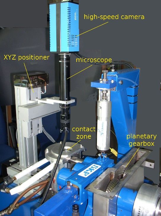
Lubricants 2019, 7, 29                                                                              2 of 17

improvements in the experimental techniques and the more sophisticated instrumentation available.
In Reference [1] a review of studies on transient conditions is presented. Sample recent studies are
reported in References [2,3], in which start-up and sudden halting conditions and the transient behavior
of transverse limited micro-grooves in EHL point contacts are investigated. Experimental tests on
non-conformal lubricated contacts under transient working conditions are commonly performed using
ball on disk test rigs. Often only one quantity is varied, usually the speed of the contacting bodies,
while the geometry and the load are kept constant. Few experimental tests have been performed on
test rigs for cam-follower contacts. The rapid variation of the operating conditions, typical of the
cam-follower contacts, makes it difficult to record the different quantities, particularly those necessary
for the evaluation of film thickness. Different methods were used for the measurement of film thickness
in cam-follower contacts. A capacitance transducer [4], thin film micro transducers [5] and an electrical
resistivity technique [6] were respectively used. Tests on real engines have been also performed, as for
instance in Reference [7], where both friction and minimum oil film thickness were measured, the latter
with a capacitance technique. However, optical interferometry has proven to be the most powerful
and detailed method for measuring film thickness and it is currently a well-established experimental
technique [8]. Two different kinds of light can normally be used: white and monochromatic light.
Many research groups use these techniques. Some examples are briefly mentioned in the following.
In Reference [9] white light interferometry was used with a digital image analysis. A spacer layer
was introduced in Reference [10] to allow measurement of very thin film. White light cannot be used
for thicknesses greater than about 1 µm; monochromatic light can be used in this case. Luo’s group
reported a method based on the relative intensity of images obtained with monochromatic light [11].
This method was further developed by using a multi-beam interference analysis in Reference [12].
In Chen and Huang’s work [13], film thickness was evaluated using monochromatic light. The method
is based on an actual intensity–thickness relation curve. Studies using dichromatic or trichromatic
light were also performed that use both color and light intensity information. Dichromatic light was
used, for instance in References [14,15]. An approach to achieve online measurement of film thickness
in a slider-on-disc contact by using dichromatic optical interferometry was reported in the work [16].
Marklund et al. described the intensity base methods with a phase measurement approach using
trichromatic light [17]. The combination of conventional chromatic interferometry with the computer
image processing methods available nowadays offers good accuracy and the possibility of analyzing a
great number of images in an automatic way [18,19] and can also be used to analyze images obtained
in line contacts [20].
      For the analysis of the large number of images recorded by a high-speed camera, a program
for automatic digital image processing was developed for point contacts by the authors’ research
group [21]. It was used for the analysis of interference images obtained in tests with constant load and
geometry but variable speed using a ball-on-disc experimental apparatus. A test rig was successively
designed and realized for a more realistic simulation of gear teeth and cam-follower contacts. The rig
was tested using circular eccentric cams [22].
      In this work, after a description of the experimental apparatus used, the main issues of the digital
image processing of interference images obtained in the line contacts are presented and discussed.
The former program, developed for point contact [21], has been improved and new versions for
calibration and successive analysis of line contacts have been realized and used for a cylindrical cam
in contact with a glass disc.

2. Materials and Methods

2.1. Experimental Test Rig
    The rig used for the experimental tests, also described in Reference [23], was entirely designed
and developed at the University of Pisa in order to investigate non-conformal lubricated contacts
between a specimen of suitable shape (usually a cam) and a counterface (usually the flat surface of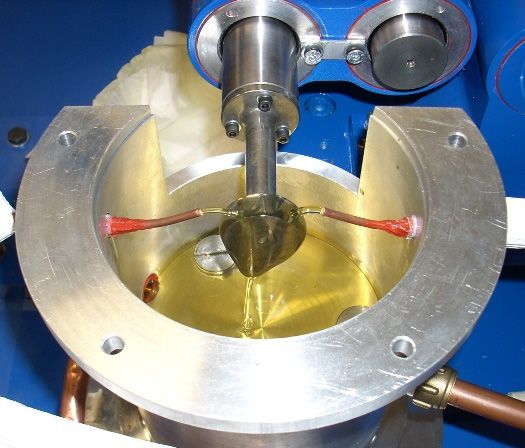
Lubricants 2019, 7, x FOR PEER REVIEW 3 of 17
Lubricants 2019, 7, 29 3 of 17
a disc, simulating a follower). The rig allows simultaneous measurements of contact force and film
thickness.
Lubricants A picture
2019, and
7, x FOR a schematic
PEER REVIEW drawing of the apparatus are shown in Figure 1. 3 of 17
(a) (b)
Figure 1. (a) Picture of the experimental apparatus for testing cam-follower contacts; (b) Schematic
drawing of the apparatus.
The camshaft is installed on a rocker arm and is driven by a planetary gearbox moved by a
brushless electric motor. The rocker arm is connected to the motor by an elastic joint. An absolute
encoder positioned after the (a) elastic joint allows the direct measurement of the (b)angular position and
velocity of the cam.
Figure
Figure 1. (a)
1. (a) Picture
Picture of the
of the experimental
experimental apparatus
apparatus for for testing
testing cam-follower
cam-follower contacts;
contacts; (b)(b) Schematic
Schematic
The contact between the cam and the plane surface of the disc occurs in the measurement unit.
drawing
drawing of the
of the apparatus.
apparatus.
This includes a system of nine annular load cells mounted in three groups, each one composed of two
tangential
The cells and one
camshaft for normal
is installed ononload.
a rockerIn thisarm way,
and alliscomponents
driven by byaofplanetary
the contact force are
gearbox measured.
moved byby a a
The camshaft is installed a rocker arm and is driven a planetary gearbox moved
Different
brushless configurations
electric motor. areThepossible
rocker byarmchanging
is the
connected loading
to thesystem
motor or
by theanmeasurement
elastic joint. group.
An In the
absolute
brushless electric motor. The rocker arm is connected to the motor by an elastic joint. An absolute
basic
encoder version the glass
positioned disc,the
after simulating
elastic the allows
joint follower, theis kept fixed
direct while the cam
measurement of of
theaxis is moving.
angular The load
position and
encoder positioned after the elastic joint allows the direct measurement the angular position and
is applied
velocity of through
the cam. an adjustable spring system. Another approach is to apply the load with weights via
velocity of the cam.
a leverThemechanism
contact mounted
between on
thethecamtheand
rocker
thethearm onsurface
plane the opposite
of of
thethe side occurs
disc of the spring;
in inthethe this configuration
measurement unit.
The contact between cam and plane surface disc occurs measurement unit.
allows
This better
includes regulation
a system of the
of nine contact
annular force,
load especially
cells mounted during the
in three calibration
groups, procedure.
each oneone composed of two
This includes a system of nine annular load cells mounted in three groups, each composed of two
The lubricant
tangential cells and isone
directly
forfor supplied
normal to the
load. contact
In In
this way, zone by an oil system.
allall
components of of
theThe temperature
contact force areis regulated
measured.
tangential cells and one normal load. this way, components the contact force are measured.
using a thermostatic
Different configurations bath. Figure 2 shows the cam used thefor obtaining the results presented in thisgroup.
work
Different configurationsare arepossible
possible by changing
by changing the loading
loading system
system or or
thethe measurement
measurement group. In the
mounted
In basic
the basicon the
versioncamshaft;
the glassthe upper part of the measurement unit with the follower is removed in this
version the glass disc, disc, simulating
simulating the follower,
the follower, is keptisfixed
kept while
fixed while
the cam theaxis
cam axis is moving.
is moving. The load
picture
The to make the cam visible.
is load is applied
applied throughthrough an adjustable
an adjustable spring system.
spring system. AnotherAnotherapproachapproach
is to apply is the
to apply
load withthe load withvia
weights
weightsThe test rig is instrumented and controlled using real-time National Instruments cRIO and
a levervia a lever mechanism
mechanism mounted on mounted
the rocker on thearmrocker
on thearm on theside
opposite opposite
of the side spring;of the
thisspring; this
configuration
LabVIEW
configuration
® software. A sampling frequency of 10 kHz is normally used during tests.
allows better regulation of the contact force, especially during the calibration procedure.
allows better regulation of the contact force, especially during the calibration procedure.
Film
The thickness and
lubricant its shape are estimated using optical interferometry. In thisThe case, the disc used
The lubricantisisdirectly
directly supplied to tothethecontact
contact zonezone by oil
by an ansystem.
oil system.The temperature temperature is
is regulated
for the
regulated experiments is made of glass coated with a thin semi-reflective layer of chromium, Cr, and a
using a using a thermostatic
thermostatic bath. Figure bath.2 Figure
shows the 2 shows
cam usedthe cam used for obtaining
for obtaining the resultsthe results presented
presented in this work
layer
thisofwork
in mounted silicon dioxide,
mounted on SiO 2, to protect the surface from abrasion and to increase the range of
thethecamshaft; the of upper part of the measurement
on the camshaft; upper part the measurement unit with theunit with is
follower the follower
removed inisthis
thicknesses
removed measurable.
picturein tothis
make picture
the camto make
visible.the cam visible.
The test rig is instrumented and controlled using real-time National Instruments cRIO and
LabVIEW® software. A sampling frequency of 10 kHz is normally used during tests.
Film thickness and its shape are estimated using optical interferometry. In this case, the disc used
for the experiments is made of glass coated with a thin semi-reflective layer of chromium, Cr, and a
layer of silicon dioxide, SiO2, to protect the surface from abrasion and to increase the range of
thicknesses measurable.
Figure 2. Picture of the top part of the measurement unit with the cover removed showing the cam
Figure 2. Picture of the top part of the measurement unit with the cover removed showing the cam
mounted on the camshaft and the final part of the oil supply system.
mounted on the camshaft and the final part of the oil supply system.
Figure 2. Picture of the top part of the measurement unit with the cover removed showing the cam
mounted on the camshaft and the final part of the oil supply system.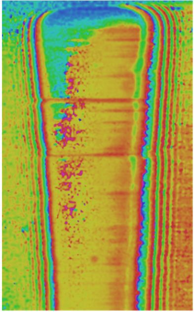
Lubricants 2019, 7, 29 4 of 17
The test rig is instrumented and controlled using real-time National Instruments cRIO and
LabVIEW® software. A sampling frequency of 10 kHz is normally used during tests.
Film thickness and its shape are estimated using optical interferometry. In this case, the disc
used for the experiments is made of glass coated with a thin semi-reflective layer of chromium, Cr,
and a layer
Lubricants 2019,of
7, silicon dioxide,
x FOR PEER REVIEWSiO2 , to protect the surface from abrasion and to increase the range
4 of of
17
thicknesses measurable.
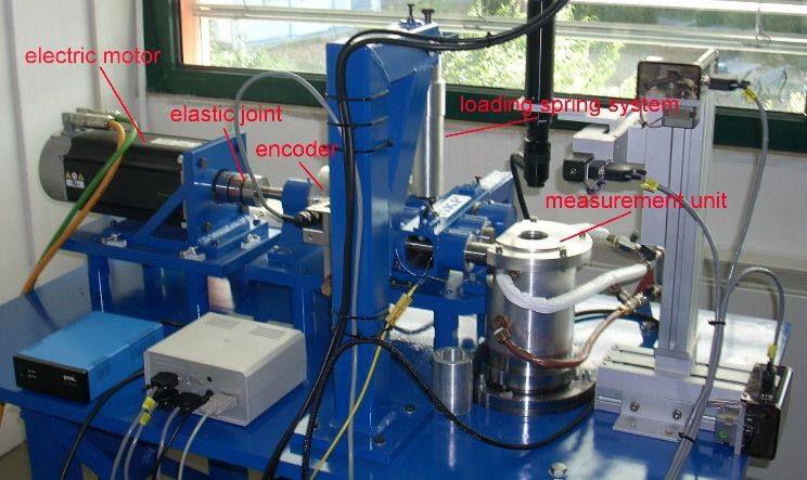
Interference
Interference images
images are
are recorded
recorded by by means
means of a microscope connected
connected to,
to, and moved
moved via, a
computer controlled
controlled XYZ positioner
positioner with
with an independent step motor for moving each axis. Detail of
the test rig
rig with
with thethe optical
opticalsystem
systemisisshown
shownininFigure
Figure3.3.
Figure 3.
Figure Picture of
3. Picture of the
the optical
optical system.
system.
A high-speed
A camera connected
high-speed camera connected toto the
the microscope
microscope allows
allows the
the recording
recording ofof interference
interference images
images
with a frame rate of up to 1000 images per second for film thickness measurements also under
with a frame rate of up to 1000 images per second for film thickness measurements also under transient transient
conditions. The
conditions. The images
images are
are recorded
recorded in
in the
the 44 GB
GB camera
camera internal memory and
internal memory and transferred
transferred toto the
the
computer successively.
computer successively.
The methodology
The methodology used
used for
forobtaining
obtainingthethefilm
filmthickness
thicknessandandshape
shapeisisdescribed
describedinindetail
detailbelow.
below.
2.2. Film Thickness Measurement Procedures
2.2. Film Thickness Measurement Procedures
It is known that a peculiarity of a cam-follower system is the movement of the contact zone during
It is known that a peculiarity of a cam-follower system is the movement of the contact zone during
the rotation of the camshaft. Even using the computer controlled XYZ positioner, depending on the
the rotation of the camshaft. Even using the computer controlled XYZ positioner, depending on the
rotational speed and on the cam’s shape, it is not easy to synchronize the target area of the microscope
rotational speed and on the cam’s shape, it is not easy to synchronize the target area of the microscope
with the contact zone. This is due to the high velocities and accelerations that the contact area can
with the contact zone. This is due to the high velocities and accelerations that the contact area can reach
reach and also due to possible vibration problems. Thus, the recording of the interference images along
and also due to possible vibration problems. Thus, the recording of the interference images along the
the contact was often achieved by repeating tests in the same working conditions, adopting different
contact was often achieved by repeating tests in the same working conditions, adopting different
positions of the microscope. Images of the contact zone were also obtained by reducing the microscope
positions of the microscope. Images of the contact zone were also obtained by reducing the microscope
magnification but the limitation is that the used magnification must be sufficient to distinguish the
magnification but the limitation is that the used magnification must be sufficient to distinguish the
interference fringes. More details of these aspects are reported in Reference [24].
interference fringes. More details of these aspects are reported in Reference [24].
Once the interference images are recorded, film thickness and shape can be evaluated by a proper
Once the interference images are recorded, film thickness and shape can be evaluated by a proper
elaboration. The methodology developed and used for the elaboration of line contact images is
elaboration. The methodology developed and used for the elaboration of line contact images is
described below. For the sake of completeness, the fundamental aspects of optical interferometry and
described below. For the sake of completeness, the fundamental aspects of optical interferometry and
the color spaces are reported before describing the procedure used.
the color spaces are reported before describing the procedure used.
2.2.1. Fundamentals of Optical Interferometry
As mentioned in the introduction, optical interferometry is a well-known powerful technique for
the estimation of the shape and thickness of non-conformal lubricated contacts, developed in the 1960s
[25]. This technique is particularly efficient under transient conditions, for which the use of other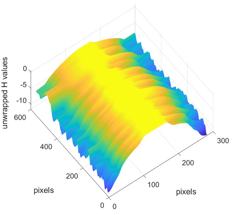
Lubricants 2019, 7, 29 5 of 17
2.2.1. Fundamentals of Optical Interferometry
As mentioned in the introduction, optical interferometry is a well-known powerful technique
for the estimation of the shape and thickness of non-conformal lubricated contacts, developed in the
1960s [25]. This technique is particularly efficient under transient conditions, for which the use of other
methods2019,
Lubricants such 7, as capacitance
x FOR PEER REVIEW or electrical resistivity is not strictly suggested. Optical interferometry 5 of 17
is typically used in ball-on-disc test rigs, but it can be applied to contacts between bodies of different
shapes (as a cylindrical cam) and a transparenttransparent surface (usually the plane surface of aa disc). disc). It is
generally
generally based
based on the interference
interference pattern
pattern created
created by the light beam reflected by a semi-reflecting
semi-reflecting
chromium layer applied to the surface of the disc and the portion of the light beam passing through the
fluid, if present, and reflected by the body. Sometimes the glass disc can be coated, on the side of the
contact, with a further layer of silicon dioxide to protect the surface from abrasion and also to increase
the measurement range towards lower thicknesses. The The two
two beams
beams cover different distances
distances and a
phase shift between the two light waves occurs. The interference interference of the two beams produces greater
visibility when the intensity of the two reflected beams is similar.
visibility similar. Since the investigation is usually
limited to the contact region, the angle formed by the incoming and the reflected beams is very little
and practically negligible.
negligible. The
The resulting
resulting wave
wave will
will have
have an amplitude
amplitude ranging
ranging from
from zero to twice the
amplitude
amplitude of the original wave, that is, destructive and constructive interference, interference, in reference to the
phase difference between the two waves. Thus, the interference pattern, consisting of bright and dark
fringes, will
will be
bevisible
visiblewhen
whenmonochromatic
monochromatic light
light is used.
is used. TheThe interference
interference pattern
pattern results,
results, in white
in white light,
light, in a graduation
in a graduation of colors
of colors due to due to theofdelay
the delay of the beams,
the beams, which iswhich
relatedis to
related to thickness.
the film the film thickness.
In FigureIn4
Figure 4 the
the basic basic principle
principle of the interferometry
of the optical optical interferometry technique
technique for fluidfor fluid
film film measurement
measurement is shown.
is shown.
Figure 4. Basic principle of optical interferometry technique.
The interference
The interference light intensity II given
light intensity given by
by the
the interference
interference of of two
two beams,
beams, with intensities II11 and
with intensities and
II22 respectively,
respectively, can
can be approximately related to the optical film thickness
be approximately related to the optical film thickness hopt h with the following
opt with the following
Equation (1),
Equation (1), taking
takinginto
intoaccount
accountthe
therefractive indices
refractive ni nofi of
indices thethe
traversed media
traversed of thickness
media hi and
of thickness the
hi and
phase difference φ caused by the reflection [26]:
the phase difference ϕ caused by the reflection [26]:
4π hopt
4πh opt + φ
p −c a−hc2opt2
a hoptcos
I = II1=+I I+
1
2 I + 2 1 I2 I e
+
2
2 I I e
1 2 cos λ +φ (1)
(1)
λ0
0
being c the attenuating coefficient of light intensity with the increase of the film thickness due to the
being caa the attenuating coefficient of light intensity with the increase of the film thickness due to the
low-coherent nature of light, λ the wavelength of the spectral light and h given by:
low-coherent nature of light, λ00 the wavelength of the spectral light and hoptopt given by:
hopt = ∑ ni hi
hopt = i ni hi
(2)
(2)
i
Monochromatic or white light can be used. Monochromatic light is characterized by a very
Monochromatic or white light can be used. Monochromatic light is characterized by a very
narrow spectrum around the wavelength λ0 which, as seen, the measurement of the film thickness
narrow spectrum around the wavelength λ0 which, as seen, the measurement of the film thickness is
is dependent on. In this case, destructive and constructive interference of the beams produces only
dependent on. In this case, destructive and constructive interference of the beams produces only dark
dark and bright fringes. With white light the changes in phase are revealed by a color transition, for
and bright fringes. With white light the changes in phase are revealed by a color transition, for
example, from yellow to red or blue to green and so forth. The interferometric image obtained with
white light is therefore characterized by a graduation of colored fringes, each one corresponding to a
value of the film thickness. These fringes are generated by the interference of beams with different
wavelengths λ and refractive index n, therefore the mathematical description of the phenomenon is
more complicated if compared with that of monochromatic light. The relationship between film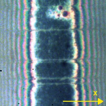
Lubricants 2019, 7, 29                                                                                6 of 17

example, from yellow to red or blue to green and so forth. The interferometric image obtained with
white light is therefore characterized by a graduation of colored fringes, each one corresponding to a
value of the film thickness. These fringes are generated by the interference of beams with different
wavelengths λ and refractive index n, therefore the mathematical description of the phenomenon
is more complicated if compared with that of monochromatic light. The relationship between film
thickness and the colors of the fringes is typically non-linear, thus a calibration table must first be
obtained. White light allows greater resolution, commonly a few nm, but it might be limited by the
human capacity to distinguish each color, which depends on color vision accuracy. To this purpose,
automatic algorithms have been developed. Anyhow, optical interferometry with white light also
presents some disadvantages concerned with the limits of the range of measurement when only the
semi-reflecting chromium layer is used: a film thickness lower than 0.1 µm leads to a dark zone tending
to black (which would mean a thickness equal to zero) and values bigger than 1 µm, due to the low
consistency of the light, leads to a vanishing of the fringes. The spacer layer of SiO2 on the glass disc is
in fact used to reduce the lower limit (and the upper), shifting downward the range of measurement to
the typical values of film thickness of EHL contacts.
      For monochromatic light tests, interference filters are often used for filtering the white light to
select just the desired wavelength. This leads to a reduction of intensity and so, compared to the
images captured using not filtered white light, longer exposure times are needed. Although it does not
represent a big issue for steady state experiments, the longer time needed to capture each image might
counteract the frame rate of the camera used for transient conditions—for cams typically in the order
of milliseconds. Therefore, digital processing of interferometric images obtained with white light has
been performed in this work.

2.2.2. Color Spaces in Optical Interferometry
     Digital image processing was historically based on RGB (Red, Green, Blue) color space. Another
way to represent any chromaticity is the HSV (Hue, Saturation, Value) color space. Some details of the
two color spaces and their relationships are reported in Appendix A.
     Either RGB or HSV color spaces can be used to analyze interferograms for EHL film thickness
measurements since they represent different ways to describe the same information. In the
interferometric images obtained with white light, the changes in phase lead to a color transition
between fringes of the same hue. Adopting Equation (1) for the resulting interference light along
the contact region, each RGB component reveals theoretically sinusoidal behavior with different
phases and frequencies. In this case, the calibration process requires particular attention since all
three color components must be taken into account. In addition, it is worth remarking that, when
RGB deconstruction is applied to interferograms for EHL film thickness measurements, a strong
sensitivity to the method used to illuminate the contact area is revealed. In particular, if the light is
not uniform, as frequently happens, the RGB components could show different values even if related
to the extent that the contact region has the same nominal film thickness. In order to overcome these
kinds of difficulties, HSV color space was adopted by the authors. The variation of the H component
is similar to an almost periodical signal ranging from 0 to 1, which is able to describe the resulting
interference light without any sensitivity in respect to saturation and brightness. It means that, in
order to evaluate the film thickness, the digital process of the image can be carried out adopting only
the H component of the fringes overcoming in this way all the problems related to the illumination
conditions of the contact area. Besides the greater insensibility to the shade and brightness of the light
and the illumination conditions, the adoption of the HSV color space also leads to a simplification
of the image processing and calibration procedures since only the H component must be analyzed
instead of three as is the case for RGB space. In Figure 5a,b sample theoretical distributions of RGB
intensities and their correspondent HSV values as a function of optical thickness are given. They have
been obtained using Equations (1) and (2) in a simple purposely developed program for the three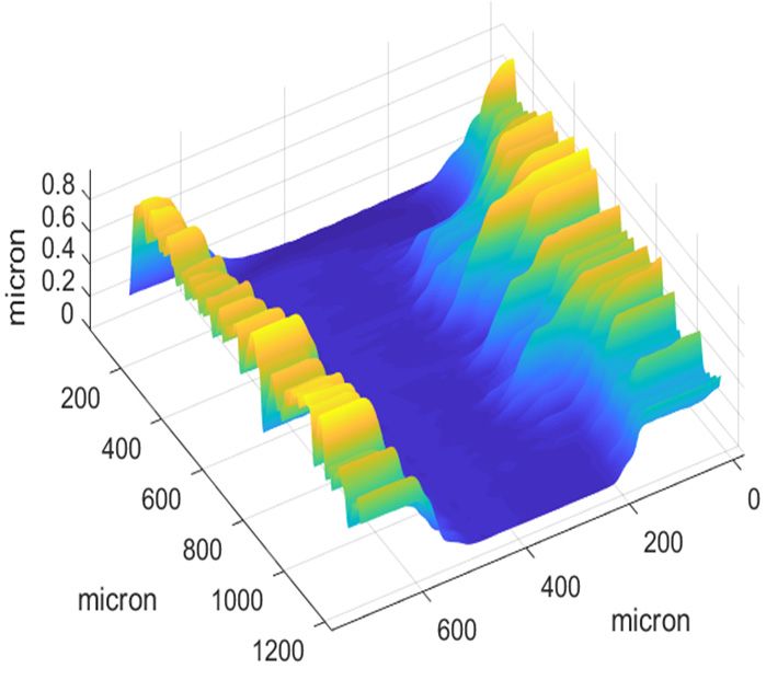
Lubricants 2019, 7, x FOR PEER REVIEW                                                                           7 of 17
 Lubricants 2019, 7, 29                                                                                           7 of 17

leading to a pixel length of 1.32 μm. Note that the image is just a portion of the cam contact zone; even
using the lower
 wavelength   foroptical magnification,
                  R, G and   B and usingit values
                                           was notsimilar
                                                   possible
                                                          toto make
                                                             those   the entire
                                                                   reported  in width of the[26].
                                                                                Reference     camH,
                                                                                                  visible
                                                                                                    S andinV
avalues
  single image.
         have been evaluated according to the conversion methods mentioned in Appendix A.

 Lubricants 2019, 7, x FOR PEER REVIEW                                                                           7 of 17

 leading to a pixel length(a)  of 1.32 µm. Note that the image is just a portion of the    (b) cam contact zone; even
 using the lower
      Figure
     Figure       (a)optical
             5.5. (a)        magnification,
                      Theoretical
                      Theoretical distributionsitofwas
                                   distributions    RGB
                                                   of  not possible
                                                        intensities
                                                      RGB             toand
                                                                    and
                                                            intensities make
                                                                        (b)  (b)the entire width
                                                                            corresponding         of thevalues
                                                                                            HSV values
                                                                                  corresponding  HSV    ascam visible
                                                                                                           function
                                                                                                                as    in
 a single image.
      of the
     functionoptical
               of the thickness.
                       optical thickness.

       The interference images obtained experimentally do not actually produce regular trends due
 to some shape irregularities such as surface roughness. In Figure 6b,c an example of RGB and HSV
 components obtained along the x-axis indicated in the interference image of Figure 6a are shown.
 The interferogram refers to the line contact occurring between a glass disc and the basic circle of a steel
 cam having a curvature radius of 14 mm, an axial width of 8 mm and an average value of the root
 mean square roughness Rq of 0.02 µm. A glass disc without the SiO2 spacer layer was used, as evident
 from the dark zone corresponding to the Hertzian contact zone. The cam was loaded against the disc
 using a load of 30 N, producing a Hertzian contact width and pressure equal to 66 µm and 73 MPa
 respectively. The image, having a size of 350 × 350 pixels, was captured adopting a magnification
                             (a)                                                       (b)
 leading to a pixel length of 1.32 µm. Note that the image is just a portion of the cam contact zone; even
 usingFigure
        the lower
               5. (a)optical magnification,
                      Theoretical             it was
                                   distributions     not possible
                                                 of RGB  intensitiestoand
                                                                       make
                                                                          (b)the entire widthHSV
                                                                              corresponding   of the cam as
                                                                                                   values visible
       function
 in a single    of the optical thickness.
              image.

               (a)                                   (b)                                       (c)
            Figure 6. (a) Interferogram; (b) corresponding RGB and (c) HSV components on x-axis.

     As expected, the variation of the H component, at least in the region close to the contact area,
assumes an almost periodical behavior. The values of S and V components have an irregular behavior.
They do not provide useful information about the changes in film thickness and are not used for the
evaluation of the distance between the two bodies in contact.

2.2.3. Elaboration of the Hue Signal
     The trend of H is similar to a periodical signal often referred to as “wrapped” hue [21]. By using
an algorithm that adds or subtracts an integer to all values subsequent to a discontinuity, a continuous
signal—usually called “unwrapped” hue—is reconstructed. The methodology is described in detail in
Reference [21](a)
                for circular point contacts. The (b) mathematical processing of the wrapped
                                                                                          (c)    hue values
may lead to an amount of noise and uncertainty in the measurement, as shown in Figure 7 where an
             Figure 6. (a) Interferogram; (b) corresponding RGB and (c) HSV components on x-axis.
example of conversion from H to the unwrapped signal, uwH, referred to the processing of the
interference image shown
      As expected,            in Figure
                           variation
                     the variation    of 6a, is
                                      of the Hshown.
                                                component,
                                                component, atat least
                                                                least in the region close
                                                                                    close to the contact
                                                                                                 contact area,
 assumes an almost periodical behavior. The values of
                                                    of SS and
                                                          and V
                                                              V components
                                                                components have
                                                                           have an
                                                                                an irregular
                                                                                    irregular behavior.
                                                                                              behavior.
 They do not provide
              provide useful information about the changes in film thickness and are not used for the
 evaluation of the
               the distance
                   distance between
                            betweenthe
                                    thetwo
                                        twobodies
                                            bodiesinincontact.
                                                       contact.

 2.2.3. Elaboration of the Hue Signal
      The trend of H is similar to a periodical signal often referred to as “wrapped” hue [21]. By using
 an algorithm that adds or subtracts an integer to all values subsequent to a discontinuity, a continuous
 signal—usually called “unwrapped” hue—is reconstructed. The methodology is described in detail in
 Reference [21] for circular point contacts. The mathematical processing of the wrapped hue values
 may lead to an amount of noise and uncertainty in the measurement, as shown in Figure 7 where an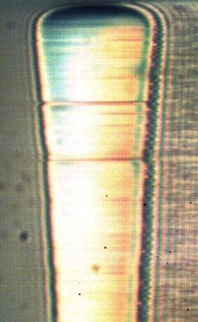
Lubricants 2019, 7, 29 8 of 17
2.2.3. Elaboration of the Hue Signal
The trend of H is similar to a periodical signal often referred to as “wrapped” hue [21]. By using
an algorithm that adds or subtracts an integer to all values subsequent to a discontinuity, a continuous
signal—usually called “unwrapped” hue—is reconstructed. The methodology is described in detail in
Reference [21] for circular point contacts. The mathematical processing of the wrapped hue values
may lead to an amount of noise and uncertainty in the measurement, as shown in Figure 7 where
an example
Lubricants 2019,of7,conversion from H to the unwrapped signal, uwH, referred to the processing of8 the
x FOR PEER REVIEW of 17
interference image shown in Figure 6a, is shown.
Figure 7. H and unwrapped signals uwH along a pixel row starting from the center of Figure 6a.
Figure 7. H and unwrapped signals uwH along a pixel row starting from the center of Figure 6a.
2.2.4. The Image Processing Program
2.2.4.The
Theimage
Imageprocessing
Processingprogram
Programdeveloped in Matlab® had already demonstrated its consistency
for circular point contacts [21]. In this case, the algorithm did not operate directly on the original
wrapped Thephase
imagemap processing
but along program
a sequencedeveloped
of radial in lines
Matlab ® had already demonstrated its consistency
at intervals of a predefined angular increment
for circular
starting frompoint contacts
the center [21].contact.
of the In this case,
In this theway,algorithm did not operate
the unwrapping procedure directly on the original
is performed by a
wrapped phase map but along a sequence of radial lines at intervals
simple mono-dimensional algorithm that unwraps the signal on each line, deciding to add or subtract of a predefined angular
increment
integer starting
values from the center
by comparing of the contact.
the differences betweenIn this way, the unwrapping
consecutive elements to aprocedure
thresholdisvalue performed
T < 1.
This pseudo-two-dimensional algorithm works properly if the threshold value is set to betono
by a simple mono-dimensional algorithm that unwraps the signal on each line, deciding add or
less
subtract integer values by comparing the differences between consecutive
than twice the maximum noise. Finally, the resulting unwrapped matrix is transformed back into the elements to a threshold
value Tcoordinates.
original < 1. This pseudo-two-dimensional algorithm works properly if the threshold value is set to
be no less
In order than twice the
to achieve themaximum
correlation noise.
between Finally,
the the resulting
fringes and the unwrapped
film thickness,matrixthe is interference
transformed
back into the original coordinates.
images are then used as input for the image process algorithm in addition to the gap values and
In orderThe
pixel length. to achieve
programthe correlation
is able to convert between the fringespattern
the interference and theinfilm thickness,
the HSV color the
space interference
allowing
operation on the single H component. The conversion from the wrapped to the unwrapped Hand
images are then used as input for the image process algorithm in addition to the gap values signalpixel
is
length. The program is able to convert the interference pattern
dependent on the threshold value T, which can be modified by the user in order to obtain, as much in the HSV color space allowing
operation
as possible,on the single Hprogression
a monotonic component.ofThe theconversion
unwrapped from thealong
signal wrapped to the unwrapped
the contact region. At H thesignal
end
is dependent on the threshold value T, which can be modified by the
of the unwrapping procedure, the user can finally choose, among the matrix of the results obtained user in order to obtain, as much
as possible,
for each patterns, a monotonic
which progression
rows must be of the unwrapped
considered signal
for the along theand
calibration contactwhichregion.
rowsAthave the end
to beof
the unwrapping procedure, the user can finally choose, among the matrix
neglected in order to consider only the progressions with a monotonic behavior of the signal; in this of the results obtained for
eachitpatterns,
way, is possible which rowsthe
to avoid must be considered
calibration for theby
being affected calibration
scratches on andthe which
glass rows
disc or have
spots to on
be
neglected
the optical in order to consider
instrumentation. Theonly
mean thevalues
progressions with aunwrapped
of the chosen monotonic behavior
signals are of put
the in
signal; in this
relation to
way, it is possible to avoid the calibration being affected by scratches
the theoretical gap between the specimen and the disc in order to obtain the calibration curve, whichon the glass disc or spots on the
opticalthe
allows instrumentation.
relation of the H The mean values
components to ofthethefilmchosen unwrapped signals are put in relation to the
thickness.
theoretical gap between the specimen and
An improvement of the mathematical processing of the wrapped the disc in order to obtainhue thehas calibration curve, which
been implemented in
allows the relation of the H components to the film thickness.
order to extend the automatic calibration procedure to the line contact. The same algorithm is used to
operate Anthe improvement
analysis of of the
line mathematical
contact images along processing of the wrapped
a sequence of parallelhue lineshasinstead
been implemented
of radial ones. in
order to extend the automatic calibration procedure to the line contact. The same algorithm is used
to operate the analysis of line contact images along a sequence of parallel lines instead of radial ones.
The distance between two consecutive lines is given by the operator as a number of pixels (one single
pixel can also be chosen). The operator also chooses a central zone of the contact from which the lines
are swept alternatively to the right and to the left. The program has also been particularly optimized
by making some procedures automatic: input data, such as working conditions, pixel length, optical
Lubricants 2019, 7, 29                                                                                                      9 of 17

The distance between two consecutive lines is given by the operator as a number of pixels (one single
pixel can also be chosen). The operator also chooses a central zone of the contact from which the lines
are swept alternatively to the right and to the left. The program has also been particularly optimized
by making some procedures automatic: input data, such as working conditions, pixel length, optical
magnification and refractive index can be automatically loaded allowing faster analyses of a large
number of images commonly recorded during tests.
     A block diagram of the program is reported in Figure 8. More details on the basic algorithms used
are reported2019,
     Lubricants     7, x FOR PEER
                in Reference      REVIEW
                                [21].                                                        9 of 17

                 Figure 8. Block
                    Figure        diagram
                           8. Block diagramofofthe
                                                the program  forthe
                                                    program for  theelaboration
                                                                     elaboration   of interference
                                                                                of interference    images.
                                                                                                images.

3. Results
    3. Results

3.1. Calibration
     3.1. Calibration
      In order  to obtain
           In order           an evaluation
                        to obtain               of theoffilm
                                    an evaluation          thethickness    starting
                                                                film thickness        from the
                                                                                   starting  frominterferograms,      a calibration
                                                                                                    the interferograms,      a
procedure    must     first be carried   out  to  relate   the  H  component       to the  distance    between
     calibration procedure must first be carried out to relate the H component to the distance between the        the  two   bodies
in contact.   The in
     two bodies     purpose
                        contact.ofThe
                                   image   calibration
                                      purpose    of imageiscalibration
                                                              to find scale
                                                                          is toand
                                                                                findoffset
                                                                                      scale factors  that
                                                                                            and offset      can be
                                                                                                         factors    used
                                                                                                                 that  can to
                                                                                                                           berelate
     used to relate the
the interferometric         interferometric
                         fringes              fringes with
                                   with the clearance         thebetween
                                                            gap    clearancethegaptwo
                                                                                    between
                                                                                        bodies.theAt
                                                                                                   two
                                                                                                     thebodies.
                                                                                                           end ofAtthe
                                                                                                                     theprocedure,
                                                                                                                          end
     of the procedure,
a calibration                a calibration
                table containing             tableintensity
                                       for each      containingcolorforthe
                                                                        each   intensity colorfilm
                                                                            corresponding         the thickness
                                                                                                       corresponding     film
                                                                                                                   is obtained.
     thickness   is obtained.
      The calibration of the interferometric images is usually performed by comparing the clearance
           The calibration of the interferometric images is usually performed by comparing the clearance
gap and contact area given by the interferograms analysis with the analogous known values given by
     gap and contact area given by the interferograms analysis with the analogous known values given
theoretical models of contact mechanics. Practically, the most common way to proceed is to capture the
     by theoretical models of contact mechanics. Practically, the most common way to proceed is to
image    of a Hertzian
     capture   the image    contact  and to then
                              of a Hertzian          correlate
                                               contact    and to thethenHcorrelate
                                                                          value ofthe  each
                                                                                          H point
                                                                                              value of
                                                                                                     of the
                                                                                                         eachinterference
                                                                                                               point of theimage
withinterference
       the theoretical      gap  given   by a   formula.     Different    formulas      are available
                     image with the theoretical gap given by a formula. Different formulas are available  for point   andforfor line
      point and for line contacts as reported for instance in Reference [27,28]. A transparent grid is normally
      used to evaluate the length of each image pixel so that the number of pixels can be converted into
      distance.
           In Figure 9 the color calibration curve obtained with the steel cam loaded against the glass disc
      is shown; the corresponding colors of the H values are given in the color bar.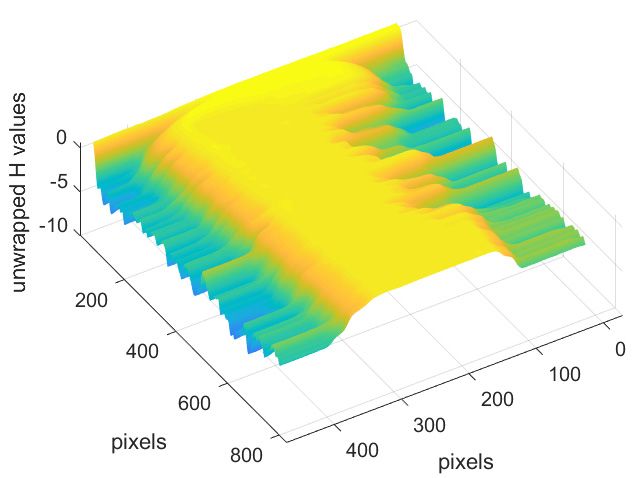
Lubricants 2019, 7, 29 10 of 17
contacts as reported for instance in Reference [27,28]. A transparent grid is normally used to evaluate
the length of each image pixel so that the number of pixels can be converted into distance.
In Figure 9 the color calibration curve obtained with the steel cam loaded against the glass disc is
shown; the2019,
Lubricants
Lubricants 2019, corresponding
7, 7, x FOR
x FOR PEERPEER colors of the H values are given in the color bar.
REVIEW
REVIEW 10 of 17 10 of 17
Figure 9. 9.
Calibration table and and
color bar for cam on glass
on disc indisc
test basic configuration.
Figure
Figure 9.Calibration
Calibrationtable
table andcolor
color bar
bar for cam
for cam on glass
glass disc inintest
test basicconfiguration.
basic configuration.
3.2.Sample
3.2. SampleResult
Resultforfor a Hertzian
a Hertzian Contact
Contact
3.2. Sample Result for a Hertzian Contact
In
Inorder
ordertotohighlight
highlight thethe
efficiency
efficiency of the
of developed
the developed algorithm, interferometric
algorithm, images images
interferometric obtainedobtained
In order to highlight the efficiency of the developed algorithm, interferometric images obtained
with
with static
static contacts
contactsbetween
betweenthe thecamcambasebasecircle
circleand
andthethedisc
discwere
werefirst
first analyzed.
analyzed.The Thecalibration
calibration curves
with static contacts between the cam base circle and the disc were first analyzed. The calibration
curves
presentedpresented
aboveabovehave have
been been
used used for the
forused
the assessment
assessment of of
thethe distancebetween
distance betweenthe the two
two bodies.
bodies.
curves
In
presented
Figure 10, an
above
example
have of
been
the
for the
application of
assessment
the procedure
of the distance
described
between
above in
thecase
the
twoofbodies.
aof a static
In In
Figure
Figure 10, an
10, example
an example of the
of application
the application of the
of procedure
the procedure described
described above
above in the
in casecase
the of a
static contact with a load of 30 N in the presence of lubricant is reported.
contact
static with
contact a load
with of
a 30 Nof
load in30the N presence
in the of lubricant
presence of is reported.
lubricant is reported.
The interferogram of Figure 10a, with a size of 213 × 563 pixels, was captured with a microscope
TheThe
magnification
interferogram
interferogram ofofFigure
leading to a pixel Figure 10a, with
length10a,
aasize
withμm.
of 1.55 size 213 ×
of 213
Theofrelated
563pixels,
× 563 pixels,was
3D unwrapped
wascaptured
captured with
with
signal (Figure
a microscope
a microscope
10c) has
magnification
magnification leading
leading to a pixel length of 1.55 µm. The related 3D unwrapped signal (Figure 10c)
been obtained using 0.1 astoa athreshold
pixel length of 1.55
value. The μm. The related
unwrapping 3D unwrapped
procedure has beensignal (Figure
performed on10c)
a has
hasbeen
been
sequence ofobtained
obtained using
using
lines crossing 0.1 0.1
the aasthreshold
a threshold
asinterferometric value.value.
fringes The The
orderunwrapping
in unwrapping
to obtain the procedure
procedure has been
gap distributionhasperformed
been
throughperformed
on a
on a sequence
sequence of of
lines lines crossing
crossing the the interferometric
interferometric fringes fringes
in order in
to order
obtain
the contact region. Figure 10d,e show the 3D representation and the contour lines of the body distance to
the obtain
gap the gap
distribution distribution
through
through theobtained
the contact
distribution contact
region.region.
Figure Figure
10d,e
by a successive 10d,e
show theshow thewhile
3D representation
3D representation
processing, and
and the contour
a comparison the
between contour
lines of thelines
body
theoretical of
and the body
distance
distribution
distance distribution
evaluated obtained
contact profile by
obtained a
along the successive
byx-axis
a successiveprocessing,
in Figureprocessing, while
10e is shown a
while comparison
a comparison
in Figure 10f. between theoretical
between theoretical andand
evaluated
evaluated contact
contact profilealong
profile alongthe thex-axis
x-axisin inFigure
Figure 10e
10e is shown
shown in in Figure
Figure10f. 10f.
(a) (b) (c)
(a) (b) 10. Cont.
Figure (c)Lubricants 2019, 7, x FOR PEER REVIEW 11 of 17
Lubricants 2019, 7, 29 11 of 17
Lubricants 2019, 7, x FOR PEER REVIEW 11 of 17
(d) (e) (f)
(d) (e) (f)
FigureFigure
10. (a)10.
Interferogram; (b) corresponding
(a) Interferogram;
Interferogram; (b)
enhanced image and (c) related 3D unwrappedsignals;
signals; (d)
Figure 10. (a) (b)corresponding
corresponding enhanced
enhanced image andand
image (c) related 3D unwrapped
(c) related (d)
3D unwrapped signals;
3D representation
3D3D of
representation the gap;
of the (e) contour lines; (f) comparison between theoretical and evaluated contact
(d) representation of gap; (e) contour
the gap; lines; lines;
(e) contour (f) comparison between
(f) comparison theoretical
between and evaluated
theoretical contact
and evaluated
profileprofile
along along
the x-axis
the reported
x-axis in subfigure
reported in (e)–static
subfigure contact–load
(e)–static contact–load30N.
30N.
contact profile along the x-axis reported in subfigure (e)—static contact–load 30N.
3.3. Sample Results
3.3. Sample for
for EHL
Results
Results Contacts
for EHL
EHL Contacts
Contacts
In orderIn order
to give
to to give
give an an idea
an idea
idea of the
of the
of the different
different
different images
images
images thatcan
that
that canbe
can beelaborated
be elaborated by
elaborated by the
by theprogram,
the program,some
program, some
some
images images
images recorded recorded
recordedatat some at
some some particular
particular
particular points
points
points during during
during the rotation
the rotation
the rotation of the same of the
of thecam same
same cam
usedcam used
for theused forforthethe
calibration,
calibration,
calibration, shown shown in
in have Figure
Figurebeen 11a, have
11a,selected.
have been been selected. A synthetic motor oil SAE 5W-40 was used asas
a a
shown in Figure 11a, A selected.
syntheticAmotorsynthetic motor
oil SAE oil SAE
5W-40 was5W-40
used as was used
a lubricant
lubricant (viscosity and pressure-viscosity coefficient 0.145 Pas and 2.2−×8 10−8 −8−Pa−1 respectively at the test
1 −1
lubricant (viscosity
(viscosity and pressure-viscosity
and pressure-viscosity coefficient
coefficient 0.145 Pas 0.145
andPas2.2and
× 2.2
10 × 10Pa Pa respectivelyatatthe
respectively the test
test
temperature of 26.7 ◦ °C). The images reported in the following refer to a test with the cam rotating at
temperature of 26.7 °C). C). The
The images
images reported
reported inin the following refer to a test with the cam rotating at
60 rpm contacting the follower with a preload of 30 N (produced by a spring when the contact occurs
60 rpm contacting
contacting the follower
follower with
with a preload of 30 N (produced by a spring when the contact occurs
on the base circle). Due to the not preload
high rotational speed, the trend of the normal force is similar to
base
on thethat
base circle).
of circle).
the Due to displacement)
lift (vertical the not high rotational speed,
shown in Figure thewith
11b, trend of the normal
a maximum value offorce is 250
about similar
N in to
that ofcorrespondence
the lift (vertical displacement) shown in Figure 11b, with a maximum value of
with the cam’s nose (position corresponding to 0° in the diagram; the abscissa starts about 250 N in
correspondence with the
withonthe cam’s nose (position corresponding to ◦
0° in the diagram; the abscissa starts
from the point thecam’s nose opposite
base circle (positiontocorresponding
the cam nose). Noteto 0 that, as reported in Reference [24],
from the
the point on the
horizontal base circleofopposite
displacement to point
the contact the cam nose). Note
corresponds withthat, as reported
the vertical velocityindivided
Reference [24],
by the
the horizontal
horizontal displacement
rotationaldisplacement
speed. of the contact
of the contact point corresponds with the vertical velocity
corresponds with the vertical velocity divided divided by the
rotational speed.
rotational speed.
(a) (b)
Figure 11. (a) Cam; (b) vertical and horizontal displacement of the contact zone.
(a) (b)
The contact positions at −49°, 0° and 125° of rotation angle, indicated by the black circles in Figure
11b, haveFigure 11. (a) Cam;
been selected (b) vertical
in order to test and
the horizontal
capabilitiesdisplacement of the
of the program in contact
zone.
zone.
very different conditions.
Also, different dimensions of the interference images have been chosen. The images were recorded
The contact
contact positionsatat −490°◦ ,and
0◦ and
125° 125
◦ of rotation
angle, angle, indicated by the black circles
with a framepositions −49°,
rate of 500 frames/s. of rotation indicated by the black circles in Figure
in Figure
11b, have 11b,
beenhave beeninselected
selected order tointest
order
the to test the capabilities
capabilities of theinprogram
of the program in very
very different different
conditions.
conditions. Also,
Also, different different dimensions
dimensions of the interference
of the interference images haveimages
beenhave been
chosen. chosen.
The imagesThe images
were were
recorded
recorded with a frame rate of 500
with a frame rate of 500 frames/s. frames/s.Lubricants 2019, 7, x FOR PEER REVIEW 12 of 17
The interference image shown in Figure 12a (683 × 1147 μm) was recorded at the inversion of
the contact motion on rising flank (rotation angle = −49°). The oil inlet is on the left of the image. The
Lubricants 2019, 7, 29 12 of 17
normal load was 165 N, the entraining velocity 47 mm/s and the curvature radius 17.6 mm. The
enhanced image and the related 3D unwrapped signals are also shown. The 3D representation of the
filminterference
The thickness andimage
the contour
shownlines
in are shown
Figure in(683
12a Figure× 12d,e
1147 while
µm) wasthe film thickness
recorded along
at the the x-
inversion of
axis reported in Figure 12e is shown in Figure 12f. ◦
the contact motion on rising flank (rotation angle = −49 ). The oil inlet is on the left of the image.
Note that the image refers to the zone close to the extremity of the cam where some contacts
The normal load was 165 N, the entraining velocity 47 mm/s and the curvature radius 17.6 mm.
between the two bodies seem to be present. In addition, the central part of the lubricated contact is
The enhanced image
not perfectly and the showing
rectangular, related 3D unwrapped
a certain taperingsignals are
that can bealso shown.
related to an The 3D representation
imperfect parallelism of
the film thickness and the contour lines are shown in Figure 12d,e while the film thickness
of the two surfaces. However, the typical EHL restriction at the exit appears in the diagrams of Figure along the
x-axis12f.
reported in Figure 12e is shown in Figure 12f.
(a) (b) (c)
(d) (e) (f)
FigureFigure 12.Interferogram
12. (a) (a) Interferogram at the
at the inversionpoint
inversion point− 49◦ ;(b)
−49°; (b)corresponding
corresponding enhanced
enhanced image; (c) related
image; (c) related
3D unwrapped
3D unwrapped signals;
signals; (d) (d)
3D3D representationof
representation ofthe
the gap;
gap; (e)
(e)contour
contourlines; (f) (f)
lines; filmfilm
thickness alongalong
thickness the the
x-axis reported in subfigure (e).
x-axis reported in subfigure (e).
In Figure 13 the cam nose being in contact with the follower (rotation angle = 0°) is shown. The
Note that the image refers to the zone close to the extremity of the cam where some contacts
normal load was 250 N, the entraining velocity 38 mm/s and the curvature radius was 6.3 mm. The
between the two bodies seem to be present. In addition, the central part of the lubricated contact is not
interference image of Figure 13a refers again to the zone close to the cam’s extremity. The bigger load
perfectly
and rectangular,
lower velocityshowing
together awith
certain tapering
the slope of thethat
camcan be related
produce to an
very low imperfect
values parallelism
of the film thicknessof the
two surfaces.
captured However, the typical
by the elaboration, EHL restriction
as shown at the exit
in the 3D diagram appears
of Figure 13b in thethe
(note diagrams
differentof Figure
full scale 12f.
In
of Figure 13 the
the vertical axis cam nosetobeing
compared that ofinFigure
contact
12d).with the follower (rotation angle = 0◦ ) is shown.
The normal load was 250 N, the entraining velocity 38 mm/s and the curvature radius was 6.3 mm.
The interference image of Figure 13a refers again to the zone close to the cam’s extremity. The bigger
load and lower velocity together with the slope of the cam produce very low values of the film
thickness captured by the elaboration, as shown in the 3D diagram of Figure 13b (note the different
full scale of the vertical axis compared to that of Figure 12d).x FOR PEER REVIEW
Lubricants 2019, 7, 29 13 of 17
Lubricants 2019, 7, x FOR PEER REVIEW 13 of 17
(a)
(a) (b)
(b)
Figure ◦
13.(a)
Figure13. (a)Interferogram at00°
Interferogramat 0°(cam
(cam nose);
nose); (b)
(b) fluid film 3D
fluid film 3D representation.
representation.
An
AnAninterference
interference
interference image
image(294
image × 318
(294
(294 pixels)
×× 318
318 recorded
pixels)
pixels) whenwhen
recorded
recorded the contact was onwas
the contact
contact the on
was basic
on thecircle
the (rotation
basic
basic circle
circle
angle = 125 ◦ ) is shown in Figure 14a. The normal load was 30 N, the entraining
(rotation angle = 125°) is shown in Figure 14a. The
(rotation angle = 125°) is shown in Figure 14a. The normalnormal load was 30 N, the entraining velocity and
30 N, the velocity
entraining44 mm/s
velocity 4444
the
mm/scurvature
mm/s and
andthe radius 14
thecurvature mm. The
curvatureradius interferogram
radius14
14mm.
mm.The refers to
Theinterferogram the central part
interferogram refers to the of the
the central contact
centralpart
partof with
ofthe dimensions
thecontact
contactwith
with
294 × 318 µm.
dimensions
dimensions 294
294× ×318
318μm.
μm.
(a)(a) (b)
(b) (c)
(c)
Figure 14.(a)
(a)Interferogram
Interferogramatat125 ◦ (b)
125°; (b)fluid
fluid film
film 3D
3D representation; (c) film
film thickness along the x and
Figure
Figure 14.
14. (a) Interferogram at 125°;; (b) fluid film 3D representation; (c) film thickness
thickness along the xx and
along the and
y axes
yy axes shown
shown in in subfigure
subfigure (a).
(a).
axes shown in subfigure (a).
The
The3D3Ddiagram
diagramofofthe
thefilm
filmthickness
thicknessisisshown
shown in
in Figure
Figure 14b and the
the trend
trend of
ofthe
thefilm
filmthickness
thickness
The 3D diagram of the film thickness is shown in Figure 14b and the trend of the film thickness
along the
along thex xand
andy yaxes
axesshown
shownininFigure
Figure14a
14aisisreported
reportedin
inFigure
Figure 14c.
14c.
along the x and y axes shown in Figure 14a is reported in Figure 14c.
4. 4.
Discussion
Discussion
4. Discussion
The
Theresults
resultspresented
presented above above showshowthat thatthe theprogram
program developed
developed for for the line
the line contacts
contacts between between
cam
cam The results presented above show that the program developed for the line contacts between cam
andand follower
follower is able
is able to to analyze
analyze very
very different
different images
images recorded
recorded during
during thetherevolution
revolutionofofthe thecam.
cam.
and follower
However, there is able
areare to
some analyze
aspects very
related different
to to
thethe images recorded
peculiarities of of
thethe during
cam-follower the revolution
contacts of
that the
make cam.
the
However, there some aspects related peculiarities cam-follower contacts that make
However,
analyses there
difficult are
and some
can aspects
explain related
some to the
irregularitiespeculiarities
in the of the
diagrams cam-follower
the analyses difficult and can explain some irregularities in the diagrams shown in the above figures.shown in the contacts
above that
figures.make
the analyses
The difficult
Thepresence
presence ofofand can explain
machining
machining marks
marks some (seeirregularities
(see forinstance
for in
instanceFigure the 12a)
Figure diagrams
12a)andand shown
surface
surface in defects
the above
defects as figures.
as well well
as theas
the The presence
presence
presence of
ofofcavitationmachining
cavitationzones zonescan marks
cancreate (see
createsome for instance
somedifficulties Figure
difficultiesfor 12a)
forthe and
theimage surface
imageanalysis. defects
analysis.Shape as well
Shapeerrors
errors as the
and
and
presence of
roughnesscan
roughness cavitation
cansignificantlyzones can
significantlyinfluence create
influencethe some
thelocal difficulties
local values
values of for
of the the
the film image
film thickness.analysis.
thickness. These Shape
These defects errors
defectscan and
canalso
also
roughness
explain
explain thethecan significantly
differences
differences between
between influence
thethe the local
theoretical
theoretical andvalues
and of the
experimental
experimental film thickness.
Hertzian
Hertzian These
profiles
profiles defects
shown
shown can also
in Figure
in Figure 10f.
explain the differences between the theoretical and experimental Hertzian
10f.The not perfect parallelism between the cam and the follower can create a zone in which the film profiles shown in Figure
10f. Theisnot
thickness notperfect parallelism
sufficient to separatebetween the cam(local
the bodies and the follower
contacts, can create
mixed or even a zone in which
boundary the film
lubrication
The
thickness not isperfect
not parallelism
sufficient to between
separate the the
bodiescam and
(localthe follower
contacts,
conditions), as shown in Figure 13. Under these conditions some wear can occur (some scratches can
mixed create
or even a zone
boundaryin which the film
lubrication are
thickness
visible is
conditions), not
in Figure sufficient
as shown
13a). On to
in Figureseparate
the other the
13. hand, bodies
Under zones (local
these conditions contacts,
with a filmsome mixed
wear can
thickness or even boundary
occurthan
greater (some lubrication
scratches
expected canarebe
conditions),
visible in as shown
Figure 13a). inOnFigure
the
present on the opposite part of the contact. 13.
other Under
hand, these
zones conditions
with a filmsome wear
thickness can occur
greater than(some scratches
expected can are
be
visible
presentin on
Contact Figure
the 13a). On
opposite
conditions thevery
part
vary other
of hand, at
thequickly
contact. zones with
certain a film positions
angular thickness of greater
the cam, than forexpected
instancecan when be
present on
close toContact the opposite
conditions
the inversion part
point vary of the
(−very contact.
49◦ ).quickly
The contact at certainpointangular
movespositions
very quickly of theafter
cam,the forinversion
instance when while
the entraining velocity is close to zero at −45 . The situation at this point is shown in Figure 15. when
Contact
close to the conditions
inversion vary
point very
(−49°). quickly
The at
contact ◦certain
point angular
moves positions
very quickly of the
after cam,
the for instance
inversion while the
Note
close to the inversion point (−49°). The contact point moves very quickly after the inversion while theYou can also read