Performance of Vehicular Visible Light Communications under the Effects of Atmospheric Turbulence with Aperture Averaging

Article

Performance of Vehicular Visible Light Communications under
the Effects of Atmospheric Turbulence with Aperture
Averaging
Elizabeth Eso 1,*, Zabih Ghassemlooy 1, Stanislav Zvanovec 2, Juna Sathian 1, Mojtaba Mansour Abadi 1
and Othman Isam Younus 1

 1 Optical Communications Research Group, Faculty of Engineering and Environment,
 Northumbria University, Newcastle‐upon‐Tyne NE1 8ST, UK; z.ghassemlooy@northumbria.ac.uk (Z.G.);
 juna.sathian@northumbria.ac.uk (J.S.); mojtaba.mansour@northumbria.ac.uk (M.M.A.);
 othman.younus@northumbria.ac.uk (O.I.Y.)
 2 Department of Electromagnetic Field, Faculty of Electrical Engineering, Czech Technical University in Prague,

 16627 Prague, Czech Republic; xzvanove@fel.cvut.cz
 * Correspondence: elizabeth.eso@northumbria.ac.uk

 Abstract: In this paper, we investigate the performance of a vehicular visible light communications
 (VVLC) link with a non‐collimated and incoherent light source (a light‐emitting diode) as the trans‐
 mitter (Tx), and two different optical receiver (Rx) types (a camera and photodiode (PD)) under
 atmospheric turbulence (AT) conditions with aperture averaging (AA). First, we present simulation
 results indicating performance improvements in the signal‐to‐noise ratio (SNR) under AT with AA
 with increasing size of the optical concentrator. Experimental investigations demonstrate the po‐
 tency of AA in mitigating the induced signal fading due to the weak to moderate AT regimes in a
Citation: Eso, E.; Ghassemlooy, Z.; VVLC system. The experimental results obtained with AA show that the link’s performance was
Zvanovec, S.; Sathian, J.; Abadi, stable in terms of the average SNR and the peak SNR for the PD and camera‐based Rx links, respec‐
M.M.; Younus, O.I. Performance of tively with

Sensors 2021, 21, 2751 2 of 17

 applications have been intensely investigated over the last decade [7,8]; however, their
 applications in outdoor environments, including VC, are still relatively new and needs
 further investigations [9,10]. In this emerging field of VC, channel modelling is critical to
 determining the performance boundaries imposed by the models and sizes of vehicles,
 infrastructure facilities, and real outdoor conditions (i.e., fog, atmospheric turbulence
 (AT), and rain/snow), which will significantly impact the performance of the link and has
 been sparsely reported in the literature [11]. In this work, the focus is on the AT, which is
 due to the varying temperature gradients and air pressure. AT is more evident on the
 road’s surface on hot days and around vehicle exhausts.
 Among the few studies reported on AT in VLC systems is [12], where the effects of
 AT on the signal quality by means of simulation considering the signal‐to‐noise ratio
 (SNR), bit error rate (BER) performance, and channel capacity metrics of the VLC system
 were investigated. The results obtained showed that there was a considerable variation in
 the BER as a function of AT levels; e.g., the BERs at a 100 m link span for two AT conditions
 of refractive index structure parameter of 1 10 and 1 10 were 3 10 and
 4 10 , respectively. In [13], the effects of AT on the BER performance of a VLC system
 were experimentally investigated under controlled laboratory conditions; however, the
 strength of AT studied was not characterized or specified. Results obtained showed a
 slight increment in the BER; e.g., under the same system parameters, the BER rose from
 3 10 to ~2 10 for a link with a 128‐quadrature amplitude modulation data format.
 The average BER of the maritime VLC system under oceanic turbulence was evaluated in
 [14], and it was found that the BER decreased with increasing aperture size and wave‐
 length, and increased with oceanic turbulence and link span. In [15], the effects of fog and
 weak AT on a VLC link with a camera‐based optical receiver (Rx) were investigated using
 Pearson’s correlation coefficient with reference to a template signal. The results obtained
 showed that under weak AT there was no significant change in the signal quality. In [11],
 we experimentally investigated the effects of higher AT strengths with AA than in [15],
 up to of 1.1 × 10–10 m−2/3 in vehicular VLC (VVLC) with a camera‐based Rx for two cam‐
 era gain factors (i.e., low and high). Results showed that the peak SNR (PSNR) perfor‐
 mance (i.e., an image quality metric) of the link was not significantly degraded by AT with
 AA for both gain factors investigated.
 Note that (i) in VLC systems, depending on applications, two types of Rxs are used:
 a photodiode (PD) and a camera. (ii) The effects of AT have been reported extensively for
 OWC links based on a coherent and a highly collimated light source (i.e., lasers) with a
 PD, as the Tx and Rx, respectively. There is still the scarcity of information on experi‐
 mental/simulation studies on the effects of AT in VVLC systems employing incoherent
 and non‐collimated light sources (i.e., LEDs) as the Txs. In this study, we extended our
 previous works by experimentally investigating the effects of AT with AA on the perfor‐
 mance of a VVLC link with a PD‐based Rx under weak to moderate AT regimes. Further‐
 more, we illustrate the effects of beam divergence of the light source on the link perfor‐
 mance considering practical VVLC system parameters. It is worth noting that optical wire‐
 less systems (visible and infrared bands) employing camera‐based Rxs offer relatively
 lower data rates compared with the high‐speed PD‐based Rxs, due to the camera frame
 rates. However, the low data rate Rb feature of optical camera communications (OCC)
 should not be seen as a problem, considering that there are many applications, including
 VC [16], indoor localization [16], Internet of Things (IoT) [16], sensor networks, motion
 capturing [17], and advertising [18], where Rb is considerably low. In OCC systems, each
 pixel at the receiving image sensor can detect signals at different wavelengths over the
 visible range, e.g., red, green, and blue (RGB), hence offering parallel detection capabili‐
 ties, an adaptive field of view feature, and even enhanced Rb using multiple‐input multi‐
 ple‐output [16,19] and artificial neural network‐based equalizers [20]. In addition, the in‐
 formation carrying light beams from different sources and many directions via the line‐
 of‐sight (LOS) [21,22], non‐LOS, and/or both paths [23] can be captured using the camera‐
 based Rxs with the extended transmission range [24] compared with the PD‐based links.

Sensors 2021, 21, 2751 3 of 17

 The remainder of the paper is organized as follows: Section 2 presents the system’s
 description, including AT parameters, models, and the VLC channel. Section 3 presents
 the simulation results. The experimental setup, signal extraction, and detection are de‐
 scribed in Section 4. In Section 5, results are presented. Finally, conclusions are given in
 Section 6.

 2. System Description
 2.1. AT Parameters and Models
 2.1.1. AT Parameters
 AT is an effect that arises from disparities in both the temperature and pressure of
 the atmosphere along the communications path. This, therefore, causes variations of the
 refractive index, which result in both amplitude and phase fluctuations of the propagating
 light beam, which leads to fading, and consequently reduced SNR and increased BER
 [25]. (in m−2/3) is most commonly used to describe the strength of AT [26], which is given
 by [27]:
 
 79 10 (1)
 
 where P represents the pressure in millibars, T is the temperature in Kelvin, and is the
 temperature structure parameter, which is related to the universal 2/3 power law of tem‐
 perature variations given as [27]:

 , ≪ ≪ 
 ⟨ ⟩ (2)
 ,0 ≪ ≪ 
 where is the separation distance between two points with temperatures of and ,
 and the inner and outer scales of the small temperature variations are denoted by and
 , respectively.
 Another important parameter, which is adopted to reflect the AT regime, is the Rytov
 variance , which indicates the irradiance fluctuations of the optical signal resulting from
 AT and is given as [27]:

 1.23 (3)

 where the wave number (λ is the wavelength), and is the link span. The AT con‐
 ditions are categorized as follows based on [27]:
 i. Weak regime, < 1;
 ii. Moderate regime, ~1;
 iii. Strong regime, 1;
 iv. Saturation regime, → ∞.
 The scintillation index is also used to quantify the normalized intensity variance
 generated by AT, and it is given by [28]:
 ⟨ ⟩
 1, (4)
 ⟨ ⟩
 where I denotes the intensity of the optical beam at the Rx, and ⟨. ⟩ represents the ensemble
 average.

 2.1.2. AT Models
 The lognormal AT model is a widely utilized model for the probability density func‐
 tion (PDF) of the randomly fluctuating signal irradiance in weak to moderate AT regimes
 due to its simplicity. This model, however, underestimates the behavior of the irradiance
 fluctuations with the increasing AT strength [27]. Consequently, to address the large‐ and

Sensors 2021, 21, 2751 4 of 17

 small‐scale scintillations in moderate to strong AT conditions, a modified Rytov theory
 was proposed in [27], where the optical channel was outlined as a function of disturbances
 arising from small and large‐scale atmospheric effects in relation to factors that behave
 like a modulation process. This model assumes that gamma distributions guide large and
 small‐scale irradiance fluctuations to develop a PDF model of the irradiance in such a way
 that the parameters used relate to the AT conditions and are still consistent with the scin‐
 tillation theory [27]. The gamma–gamma (GG) model is a suitable model covering the
 weak to strong AT regime, and its PDF is given by [29,30]:
 ∝
 2 ∝ ∝
 (5)
 2 , 0
 
 where α and β are the effective numbers of large and small‐scale eddies of the scattering
 process, respectively. . and . denote the gamma function and the modified Bes‐
 sel function of the second order (α − β), respectively. For the plane wave radiation at the
 Rx, α and β are given by, respectively [27]:
 . ⁄
 1/ 1 , (6)
 . ⁄
 1/ 1 (7)

 where 1 1.11 and 1 0.69 .

 Alternatively, a generalized statistical model of the Malaga distribution can be used
 to model the irradiance fluctuations under all AT conditions [31]. The merits of this model
 include a closed‐form and a mathematically tractable expression for the fundamental
 channel statistics under all AT regimes, as well as unifying most of the pre‐existing statis‐
 tical models for irradiance fluctuations [31,32]. The PDF of the Malaga distribution is
 given as [32]:

 2 , 0 (8)
 Ω

 Where

 ∝ ∝
 ∝
 ≜ ∝
 ’ (9)
 ∝

 1 Ω Ω (10)
 ≜ ,
 1 1 ! 

 Ω ≜Ω 2 2 2 Ωcos φ φ (11)
 where 2 is the average power of the total scatter components, is a natural number
 representing the amount of AT, 0 1 is the amount of scattering power that is
 coupled to the LOS component, is related to the effective number of large scale cells of
 the scattering process, Ω is the average power of the LOS component, = 2 ( 1 , and
 φ , φ are the LOS phases and coupled to LOS components.

 2.2. VLC System
 For a VLC system, the received signal via the LOS path is given by [33]:
 ℛ ⊗ ℎ , (12)

Sensors 2021, 21, 2751 5 of 17

 where ℛ is the responsivity of the PD; n(t) denotes the additive white Gaussian noise, in‐
 cluding the sunlight noise, thermal noise, signal, and dark current‐related shot noise
 sources with zero mean and a total variance ; and h(t) represents the channel impulse
 response, which is related to the channel DC gain as given by [33]:

 ℎ d . (13)

 Note that the daytime ambient sunlight‐induced shot noise is the dominant noise
 source in VVLC, which is expressed as [34,35]:
 2 (14)
 Where is the electron charge, and is the system’s bandwidth. Note that for the on–
 off keying (OOK) data format, ⁄2 [36]. is the ambient noise current, and dur‐
 ing the daytime , which can be expressed as [37]:

 cos ℛ , (15)

 where is the active area the PD; is the incidence angle; is the solar irradiance; 
 and are the integration limits, i.e., the wavelength band, which are 405–690 nm for the
 visible range; and represent the gain of the optical concentrator (OC) and the trans‐
 mittance of the optical filter, respectively. Additionally, the thermal noise, signal‐depend‐
 ent shot noise at the PD, the PD’s dark current noise, and consequently the total noise
 variances are given, respectively, as [33,36,38]:
 4 
 , (16)
 
 2 ℛ (17)
 2 , (18)
 (19)
 where is Boltzmann’s constant, is the absolute temperature in Kelvin, is the load
 resistance, and is the dark current. denotes the average optical transmit power, and
 H for the LOS VVLC link with a symmetrical Tx light radiation pattern can be expressed
 as [33]:
 1 
 cos cos , 0 ∅
 2 (20)
 0, ∅
 where denotes the irradiance angle, ∅ is the angular field of view (AFOV) semi‐angle of
 the Rx, and is the distance between the Tx and Rx. The of a non‐imaging OC can be
 expressed as ⁄ [39], where ⁄4) is the collection area of the non‐
 imaging OC, is the diameter of the OC, and m represents Lambertian order of emission
 of the Tx, which is given by [33]:
 ln2
 , (21)
 ln cos ⁄

 where ⁄ is the half power angle. Lambertian radiant intensity is expressed as [33]:
 1
 cos , (22)
 2 
 The average SNR without and with the AT for a point Rx (i.e., with no OC) for OOK
 signaling are given, respectively, as [27,33]:

Sensors 2021, 21, 2751 6 of 17

 ℛ 0
 SNR 0 , (23)
 2 0
 SNR
 SNR 0 , (24)
 1 0 SNR
 Using an OC (i.e., aperture averaging), the average SNR with and without the AT are
 given as [27,33]:
 ℛ 
 SNR , (25)
 2 
 SNR 
 SNR , (26)
 1 SNR 
 is the variance of the intensity fluctuations for an OC of D, and 0 is the
 scintillation index for a point Rx ( 0). For the plane wave propagation with the outer‐
 and inner‐scale temperature variation parameters of ∞ and 0, respectively, can
 be expressed as [40]:

 0.49 0.51 1 0.69 
 exp 1, (27)
 1 0.653 1.11 1 0.9 0.621 

 where .
 The average BER is given as [33]:
 BER √SNR , (28)
 where is the ‐function used for the calculation of the tail probability of the standard
 Gaussian distribution given by [33]:
 1
 , (29)
 √2 
 Next, with (23), (24), and (28) the average BER of the link under AT can be expressed
 as [27,33]:
 ℛ 
 BER . (30)
 2 ℛ 
 In OCC systems, an image quality metric known as the PSNR is used for assessing
 the link’s quality, which is given by [41]:
 
 PSNR 10log , (31)
 MSE
 where = 255 for the grayscale image (i.e., the maximum possible pixel value), and MSE
 is the pixel luminance mean squared error, which is defined by [16]:

 1
 MSE , (32)
 
 where are the pixel values for the transmitted symbols, (in this work we have obtained
 from captured images at approximately a zero distance from the Tx, i.e., without con‐
 sidering the channel impact), are the average pixel values for the received symbols, n
 is the number of rows (i.e., the on and off states of the Tx for OOK signaling scheme), and
 j is the pixel’s row index number.

Sensors 2021, 21, 2751 7 of 17

 3. Simulation of AT Effects with AA
 To reduce the degradation of the propagating signal due to AT effects, a number of
 options have been proposed, including (i) spatial diversity with adequate spacing [42],
 which is not suitable in VVLC since the width of vehicles is within the range 1.5–2.0 m
 [43]; (ii) beam width optimization [44], where the radiation pattern of the beam is altered,
 which is also impractical in VVLC since vehicles will have different HL and TL shapes,
 dimensions, and radiation patterns; in addition, including additional optics in HL and TL
 or in another infrastructure lighting to change the radiation properties may not be a viable
 option; (iii) complex modulation and coding [45]; and (iv) AA technique [40], which is a
 simple method and can be easily achieved in a VVLC system on the Rx side. AA involves
 using a lens in front of a small optical detector, thereby increasing the collection area of
 the Rx, hence lowering the effects of AT and spatially filtering the high fluctuations of the
 received optical beam. The AA factor is expressed as [40] .
 We present here simulation results for the degree of light collimation (i.e., the beam
 divergence angle ⁄ ) of a light source with AA and under weak to moderate turbulence
 conditions using Equations (14)–(30). Using the key system parameters given in Table 1,
 first, we investigate the dependency of the mean BER performance on ⁄ of the Tx with‐
 out and with weak to moderate AT (i.e., = 0.5) for a range of inter‐vehicle distances
 with D of 25 mm under sunlight, as depicted in Figure 1. The plot shows that the BER
 increased with the inter‐vehicle distance crossing the forward error correction (FEC)
 limit of 3.8 10 at of 50 and 64 m for ⁄ of 50°, with and without AT, respectively.
 Moreover, for the of 40 m, the BERs without and with AT are 4.3 10 and 3.1 10
 for ⁄ = 60°; and 1.0 10 and 1.0 10 for ⁄ = 30°, respectively.

 Table 1. Key simulation parameters.

 Parameter Value
 PD responsivity ℛ 0.43 A/W
 Rytov variance 0.1–1
 Beam divergence angle (half power angle) ⁄ 30–60°
 Inter‐vehicle distance 10–100 m
 Bandwidth B 5 MHz
 Optical transmit power 0.5 W
 Diameter of OC D 20–35 mm
 Tx wavelength 630 nm
 PD area 0.75 10 m
 Diameter of PD 9.8 10 m
 Incidence angle 0°
 Absolute temperature 298 K
 Solar irradiance 100 W/m2
 Load resistance 50 ohms
 PD dark current 5 nA
 Transmission coefficient of filter 1

 Furthermore, we investigate the average SNR as a function of ⁄ for a range of D
 under weak to moderate AT (i.e., = 0.5) and of 50 m, as shown in Figure 2a. Addi‐
 tionally, shown for reference is the SNR plot for the case with no AT and OC. As shown,
 the SNR plots are almost independent of ⁄ with AA but increases with D under AT.
 E.g., for D = 30 mm and ⁄ = 20, 30, and 40°, the SNRs were 23.9, 23.8, and 23.4 dB, re‐
 spectively. Next, the average SNR performance gain achieved by AA under AT can be
 expressed as:

Sensors 2021, 21, 2751 8 of 17

 SNR 1 0 SNR 0 SNR 
 , (33)
 SNR 0 1 SNR SNR 0
 where SNR and SNR 0 are the mean SNRs with and without AA under AT. Fig‐
 ure 2b shows as a function of D for a range of , where = 50 m and ⁄ = 45°.
 It is apparent that increases with a decrease in AT strength) and an increase
 in D. For example, at = 0.4, the s were 14.3, 17.5, 19.9, and 21.8 dB for D of 20,
 25, 30, and 35 mm, respectively.

 100

 10-1

 10-2

 10-3

 10-4

 10-5

 10-6
 10 20 30 40 50 60 70 80 90 100
 Link span (m)
 Figure 1. Bit error rate (BER) performance without and with weak to moderate atmospheric turbu‐
 lence (AT) conditions for a range of inter‐vehicle distances and ⁄ .

 50
 no AT & no OC
 45 with AT & no AA
 with AT & D=20 mm
 40 with AT & D=25 mm
 with AT & D=30 mm
 35 with AT & D=35 mm

 30
 SNR (dB)

 25

 20

 15

 10

 5

 0
 10 20 30 40 50 60
 o
 1/2
 ( )
 (a)

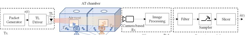
Sensors 2021, 21, 2751 9 of 17

 30 2
 R
 =0.1
 2
 =0.4
 R
 25 2
 =0.7
 R
 2
 =1.0
 R
 20

 G SNR-AA (dB)
 15

 10

 5

 0
 5 10 15 20 25 30 35
 D (mm)
 (b)

 Figure 2. (a) Effects of aperture averaging (AA) for a range of D on the signal to noise ratio (SNR)
 performance as a function of ⁄ , and (b) the SNR gain as a function of D with AA for a range of .

 4. System Setup
 4.1. Experimental Testbed
 Experimental investigation of AT with AA was carried out. The schematic block di‐
 agram of the proposed VVLC system with the PD and camera‐based Rxs with AA and
 under AT is depicted in Figure 3. Rx1 was composed of a camera (Thorlabs DCC1645C‐
 HQ) with a lens (Computar MLH‐10X), and Rx2 was composed of a PD (PDA100A2) and
 a convex lens. An indoor laboratory atmospheric chamber was used to simulate the out‐
 door AT, as proposed in [26]. At the Tx, data packets of length 90 bits in the non‐return to
 zero OOK format were generated using an arbitrary waveform generator, the output of
 which was used for intensity modulation of the TL (Truck‐trailer DACA08712AM) via the
 driver module. The intensity‐modulated light beam transmitted over a dedicated atmos‐
 pheric chamber was captured at the Rxs. AT was generated within the chamber by vary‐
 ing the temperature along the transmission path using hot/cold fans. Seventeen tempera‐
 ture sensors were used within the chamber to measure the temperature distribution. The
 key experimental parameters adopted in the proposed system are listed in Table 2.

 Figure 3. Setup of experimental investigation on AT effects on the vehicular visible light communications (VVLC) link
 with: (a) the camera and (b) the photodiode (PD) optical receiver (Rx).

Sensors 2021, 21, 2751 10 of 17

 Table 2. Key parameters of the experiment.

 Description Value
 Tx peak wavelength 630 nm
 Tx Tx bias current 98 mA
 Transmit power 32.4 mW
 Thorlabs PDA100A2
 Responsivity 0.43 A/W at 630 nm
 PD area 0.75 10 m
 PD Rx Bandwidth @ 0 dB gain 11 MHz
 Noise equivalent power @ 960 nm 7.17 10 W√Hz
 Lens focal length f 25 mm
 Lens diameter D 25 mm
 Thorlabs DCC1645C‐HQ
 Camera shutter speed 600 μs
 Camera gain factors 1.07 , 3.96
 Lens focal length f 130 mm
 Camera Rx Lens aperture f5.6
 Samples per frame 2588
 Pixel clock 10 MHz
 Camera frame rate 6.25 fps
 Camera resolution 1280 × 1024
 Data format NRZ‐OOK
 Packet Generator Packet generator sample rate 11.125 kHz
 Number of samples per bit 10
 Channel AT chamber dimension 33 × 35 × 720 cm3

 4.2. Signal Extraction
 On the Rx side, the captured regenerated electrical signals from PD and camera‐
 based Rxs were processed offline in MATLAB®. Algorithm 1 shows the image processing
 algorithm for signal extraction for the camera Rx. For Rx1, a rolling shutter (RS)‐based
 camera was employed; the captured frames’ RGB components were converted to gray‐
 scale for both the data and calibration video streams following pixelation (i.e., digitizing
 the image to obtain the pixel value) using Algorithm 1. Note that the data and calibration
 video streams represent the captured transmitted data and the template shape of the Tx
 (i.e., the DC gain), respectively. The latter was used for the intensity compensation (i.e.,
 normalization) of the data video frames. Subsequently, the captured frames were then
 normalized over the rows to obtain the received signal waveform as illustrated in Figure
 4a,b, which shows an example of a captured frame before and after normalization, respec‐
 tively. Note that in RS‐based cameras, the camera sequentially integrates incoming light
 illuminating the camera pixels, thereby offering flicker‐free transmission with increased
 data rates.

 Algorithm 1. The image processing algorithm for signal extraction.
 Input: Captured data frames and the DC signal only frames 
 Output: 
 1 For each do
 Read 3 sized frame = [ , , . The RGB components of
 denoted as , , , , , , re‐
 2
 spectively, i = 1, 2, …, U and j = 1, 2, …, V represents the pixels indices of cap‐
 tured frame, and c = 1, 2, 3.

Sensors 2021, 21, 2751 11 of 17

 Apply grayscale conversion by calibrating the RGB components
 3
 , , and together over c, resulting .
 Accumulate intensities for all pixels at each row 
 4
 where ∑ .
 5 Estimate the averaged DC value ̅ by repeating previous steps on .
 6 Calibrate s with respect to the averaged DC value ⁄ ̅
 7 Resample with respect to the packet length
 8 End.
 104
 3.5
 Captured signal
 DC gain

 3

 Cumulative received intensity
 2.5

 2

 1.5

 1
 0 200 400 600 800 1000
 Pixel row number
 (a)
 1

 0.9

 0.8

 0.7

 0.6

 0.5

 0.4
 0 200 400 600 800 1000
 Pixel row number
 (b)
 Figure 4. An example of a captured image frame for the camera‐based Rx: (a) before and (b) after
 intensity normalization.

 For Rx2, i.e., the PD‐based Rx, the signal was captured using a digital oscilloscope
 (Agilent Technologies DSO9254A) for offline processing in MATLAB®. For both Rxs, the
 detection process included (i) a low pass Butterworth filter (first‐order with a normalized
 cut off frequency wn of 0.1 rad/sample for the PD received signals, and a third‐order with
 wn = 0.25 rad/sample for the camera signals are used); (ii) a sampler (sampling at the
 middle of the samples received for each bit and at an interval of ; and (iii) a slicer

Sensors 2021, 21, 2751 12 of 17

 (with the threshold level set to the mean value of the signal, and for Rx1 this was done per
 frame).

 5. Results and Discussions
 5.1. Camera‐Based Rx
 Measurements were carried out for link with and without AT for the camera shutter
 speed of 600 μs and the low and high gain factors of 1.07 times ( ) and 3.96 , respectively.
 Note that the camera‐based Rx had a gain factor in the range of 1 to 4.27 ; where 1 and
 4.27 imply no gain and the maximum gain, respectively. Consequently, to assess the link
 quality, we have used the PSNR as given in Equations (31) and (32). Figure 5 shows the
 PSNR versus with AA for the low and high gain factors. It illustrates that with AA (i)
 the PSNR is almost independent of AT with a marginal drop for the link with a gain factor
 of 3.96 ; and (ii) there was a PSNR gain of ~7 dB for the captured frames at the higher
 gain factor.
 Note that the corresponding for the experimentally measured for different AT
 strengths were determined using Equation (3) for equal to the length of the AT chamber
 (7.2 m), which are given in Table 3. Note that both the image contrast and its brightness
 increase with the camera’s gain factor, since the signal is amplified prior to the digitizing
 process [46]. The choice of the two gain factors (i.e., low and high) is used to illustrate the
 image contrast/brightness effects under AT.

 Table 3. for corresponding values measured in the experiments.

 ( ⁄ ) 
 3.9 10 0.2619
 PD 7.9 10 0.5304
 1.0 10 0.6714
 3.6 10 0.2417
 3.9 10 0.2619
 7.9 10 0.5304
 Camera
 8.0 10 0.5371
 8.3 10 0.5573
 1.1 10 0.7386
 PSNR (dB)

 Figure 5. The peak SNR (PSNR) as a function of for the two gain factors.

Sensors 2021, 21, 2751 13 of 17

 Figure 6 shows the captured received signal waveforms prior to being applied to the
 detection module for different AT strengths with AA after normalization. The received
 signal employing a higher gain factor showed improved PSNR performance and higher
 received signal intensity with lower intensity fluctuations. The BER measured was less
 than the target BER of 10–4 for all the link scenarios considered. Furthermore, the histo‐
 gram plots prior to the detection module are depicted in Figure 7a–d, which illustrate the
 distributions of discrete intensity levels of the captured images within the range of 0 to 1
 for the captured image frames per link. Figure 7e shows the histogram for the sampled
 received intensity levels of Figure 7a at the output of the sampler (i.e., within the detection
 module). Note the slight overlap between the received intensities for the bits 0 and 1 in
 Figure 7a–d, which was due to the slow rise‐time of the captured on and off states of the
 Tx. This was because of the transition between different illumination levels brought about
 by the sampling process in the RS‐based camera [20]. Consequently, this happened at the
 transition edges; however, for the proposed detection module, the sampling takes place
 at the center of the received samples per bit; hence the system’s performance was not de‐
 graded and bits 0 are 1 were clearly distinguishable, as in Figure 7e. Moreover, it can be
 observed that the link with a higher gain factor (i.e., Figure 7c,d) had higher peak counts
 than Figure 7a,b with the low gain factor.

 1.1

 1

 0.9

 0.8

 0.7

 0.6

 0.5
 0 100 200 300 400 500
 Data samples
 (a)
 1.1

 1

 0.9

 0.8

 0.7

 0.6

 0.5
 0 100 200 300 400 500
 Data samples
 (b)
 Figure 6. Waveforms of Rx data at varying AT strengths for the gain factors of: (a) 1.07 and (b)
 3.96 [11].

Sensors 2021, 21, 2751 14 of 17

 (a) (b)
 10 4
 6

 4

 2

 0
 0.4 0.6 0.8 1
 Received intensity (a.u.)
 (c) (d)

 (e)
 Figure 7. Camera Rx histogram plot: prior detection module for (a) gain 1.07 with no AT, (b) gain
 1.07 with the highest AT scenario, = 1.0 10 m ⁄ , (c) gain 3.96 with no AT, and (d) gain
 3.96 , with the highest AT scenario = 1.1 10 m ⁄ ; and (e) output of the sampler for (a).

 5.2. PD‐Based Rx
 For the link with AA and the PD‐based Rx, we have measured the SNR of the cap‐
 tured signals and produced histogram plots for bits 0 and 1, i.e., the signal distribution
 profile for the channel with and without AT, as shown in Figure 8, prior to the detection
 module. From the results obtained, (i) the histogram plot shows a clear distinction be‐
 tween the received signal for bits 0 and 1; and the average SNR is independent of the weak
 to moderate AT (with only ~0.1 dB of SNR penalty compared with the clear channel with
 OC). Thus, this demonstrates that AA can effectively combat the induced signal fading
 due to AT for the VVLC systems under weak to moderate turbulence regimes.

Sensors 2021, 21, 2751 15 of 17

 SNR = 12.7 dB SNR = 12.6 dB

 (a) (b)
 SNR = 12.6 dB SNR = 12.6 dB

 (c) (d)
 Figure 8. PD Rx histogram plot for (a) a clear channel and channels with AT conditions of (b) =
 3.9 10 m ⁄ , (c) = 7.9 10 m ⁄ , and (d) = 1.0 10 m ⁄ .

 6. Conclusions
 First, we presented the simulation results for a VVLC system with aperture averaging
 to mitigate the signal degradation due to atmospheric turbulence. The results obtained
 showed a performance improvement in terms of the SNR under weak to moderate turbu‐
 lence regimes with an increasing diameter of the receiver lens. Moreover, results also re‐
 vealed that, for an increasing beam divergence angle (half power angle) the inter‐link BER
 degradation decreased with and without turbulence. Furthermore, we experimentally in‐
 vestigated the effects of aperture averaging for the VVLC link under turbulence using an
 LED‐based vehicle’s taillight. The results obtained showed that with the aperture averag‐
 ing there was no significant system performance degradation under atmospheric turbu‐
 lence, whereas both PSNR and SNR dropped by 0.7 and 0.1 dB for the camera and PD‐
 Rxs, respectively, compared with the clear channel. Finally, we demonstrated that in
 VVLC systems employing incoherent non‐collimated LED light sources as the Tx, the ap‐
 erture averaging method proved to be very potent at mitigating weak to moderate turbu‐
 lence regimes, and in fact also increased the optical power density of the received signal
 at the Rx.

Sensors 2021, 21, 2751 16 of 17

 Author Contributions: Conceptualization, E.E.; methodology, E.E.; software, E.E. and M.M.A.;
 validation, E.E., Z.G., M.M.A., and S.Z., investigation, E.E.; resources, Z.G. and M.M.A.; writing—
 original draft preparation, E.E.; writing—review and editing, E.E., Z.G., S.Z., J.S., O.I.Y., and
 M.M.A.; supervision, Z.G.; funding acquisition, Z.G. All authors have read and agreed to the pub‐
 lished version of the manuscript.
 Funding: The work was supported by the European Union’s Horizon 2020 Research and Innova‐
 tion Programme under the Marie Sklodowska–Curie grant agreement number 764461 (VISION)
 and the EU COST Action on Newfocus (CA19111), and partly by CELSA project PICNIC.
 Institutional Review Board Statement: Not applicable.
 Informed Consent Statement: Not applicable.
 Data Availability Statement: The data presented in this study are available on request from the
 corresponding author.
 Conflicts of Interest: The authors declare no conflict of interest. The funders had no role in the
 design of the study; in the collection, analyses, or interpretation of data; in the writing of the man‐
 uscript, or in the decision to publish the results.

References
1. Gao, S.; Lim, A.; Bevly, D. An empirical study of DSRC V2V performance in truck platooning scenarios. Digit. Commun. Netw.
 2016, 2, 233–244.
2. Shen, W.‐H.; Tsai, H.‐M. Testing vehicle‐to‐vehicle visible light communications in real‐world driving scenarios. In Proceedings
 of the 2017 IEEE Vehicular Networking Conference (VNC), Torino, Italy, 27–29 November 2017; pp. 187–194.
3. Vivek, N.; Srikanth, S.V.; Saurabh, P.; Vamsi, T.P.; Raju, K. On field performance analysis of IEEE 802.11p and WAVE protocol
 stack for V2V & V2I communication. In Proceedings of the International Conference on Information Communication and Em‐
 bedded Systems (ICICES2014), Chennai, India, 27–28 February 2014; pp. 1–6.
4. Xu, Z.; Li, X.; Zhao, X.; Zhang, M.H.; Wang, Z. DSRC versus 4G‐LTE for Connected Vehicle Applications: A Study on Field
 Experiments of Vehicular Communication Performance. J. Adv. Transp. 2017, 2017, 1–10.
5. Bazzi, A.; Masini, B.M.; Zanella, A.; Calisti, A. Visible light communications as a complementary technology for the internet of
 vehicles. Comput. Commun. 2016, 93, 39–51.
6. Car Lighting District. Halogen vs. HID vs. LED—Which is Best? 2018. Available online: https://www.carlightingdis‐
 trict.com/blogs/news/halogen‐vs‐hid‐vs‐led‐which‐is‐best (accessed on 1 April 2019).
7. Karunatilaka, D.; Zafar, F.; Kalavally, V.; Parthiban, R. LED Based Indoor Visible Light Communications: State of the Art. IEEE
 Commun. Surv. Tutor. 2015, 17, 1649–1678.
8. Pathak, P.H.; Feng, X.; Hu, P.; Mohapatra, P. Visible Light Communication, Networking, and Sensing: A Survey, Potential and
 Challenges. IEEE Commun. Surv. Tutor. 2015, 17, 2047–2077.
9. Cailean, A.M.; Dimian, M. Impact of IEEE 802.15. 7 Standard on Visible Light Communications Usage In Automotive Applica‐
 tions. IEEE Commun. Mag. 2017, 55, 169–175.
10. Cailean, A.‐M.; Dimian, M. Current Challenges for Visible Light Communications Usage in Vehicle Applications: A Survey.
 IEEE Commun. Surv. Tutor. 2017, 19, 2681–2703, doi:10.1109/comst.2017.2706940.
11. Eso, E.; Younus, O.I.; Ghassemlooy, Z.; Zvanovec, S.; Abadi, M.M. Performances of Optical Camera‐based Vehicular Commu‐
 nications under Turbulence Conditions. In Proceedings of the 2020 12th International Symposium on Communication Systems,
 Networks and Digital Signal Processing (CSNDSP), Porto, Portugal, 20–22 July 2020; pp. 1–5.
12. Guo, L.‐D.; Cheng, M.‐J. Visible light propagation characteristics under turbulent atmosphere and its impact on communication
 performance of traffic system. In Proceedings of the 14th National Conference on Laser Technology and Optoelectronics (LTO
 2019), 2019, Shanghai, China, 17 May 2019; Volume 11170, p. 1117047.
13. Martinek, R.; Danys, L.; Jaros, R. Visible Light Communication System Based on Software Defined Radio: Performance Study
 of Intelligent Transportation and Indoor Applications. Electron. 2019, 8, 433, doi:10.3390/electronics8040433.
14. Zheng, X.‐T.; Guo, L.‐X.; Cheng, M.‐J.; Li, J.‐T. Average BER of Maritime Visible Light Communication System in Atmospheric
 Turbulent Channel *. In Proceedings of the 2018 Cross Strait Quad‐Regional Radio Science and Wireless Technology Conference
 (CSQRWC), Xuzhou, China, 21–24 July 2018; pp. 1–3, doi:10.1109/CSQRWC.2018.8455332.
15. Matus, V.; Eso, E.; Teli, S.R.; Perez‐Jimenez, R.; Zvanovec, S. Experimentally Derived Feasibility of Optical Camera Communi‐
 cations under Turbulence and Fog Conditions. Sensors 2020, 20, 757.
16. Cahyadi, W.A.; Chung, Y.H.; Ghassemlooy, Z.; Hassan, N.B. Optical Camera Communications: Principles, Modulations, Poten‐
 tial and Challenges. Electronics 2020, 9, 1339.
17. Teli, S.R.; Zvanovec, S.; Ghassemlooy, Z. Performance evaluation of neural network assisted motion detection schemes imple‐
 mented within indoor optical camera based communications. Opt. Express 2019, 27, 24082–24092.
18. Saeed, N.; Guo, S.; Park, K.‐H.; Al‐Naffouri, T.Y.; Alouini, M.‐S. Optical camera communications: Survey, use cases, challenges,
 and future trends. Phys. Commun. 2019, 37, 100900.

Sensors 2021, 21, 2751 17 of 17

19. Teli, S.R.; Matus, V.; Zvanovec, S.; Perez‐Jimenez, R.; Vitek, S.; Ghassemlooy, Z. Optical Camera Communications for IoT–
 Rolling‐Shutter Based MIMO Scheme with Grouped LED Array Transmitter. Sensors 2020, 20, 3361.
20. Younus. O.I.; Hassan, N.B.; Ghassemlooy, Z.; Haigh, P.A.; Zvanovec, S.; Alves, L.N.; Le Minh, H. Data Rate Enhancement in
 Optical Camera Communications Using an Artificial Neural Network Equaliser. IEEE Access 2020, 8, 42656–42665.
21. Lee, H.‐Y.; Lin, H.‐M.; Wei, Y.‐L.; Wu, H.‐I.; Tsai, H.‐M.; Lin, K.C.‐J. RollingLight: Enabling Line‐of‐Sight Light‐to‐Camera Com‐
 munications. In Proceedings of the 13th Annual International Conference on Mobile Systems, Applications, and Services, Flor‐
 ence, Italy, 19–22 May 2015; pp. 167–180.
22. Nguyen, T.; Islam, A.; Hossan, T.; Jang, Y.M. Current Status and Performance Analysis of Optical Camera Communication
 Technologies for 5G Networks. IEEE Access 2017, 5, 4574–4594.
23. Hassan, N.B.; Ghassemlooy, Z.; Zvanovec, S.; Biagi, M.; Vegni, A.M.; Zhang, M.; Luo, P. Non‐Line‐of‐Sight MIMO Space‐Time
 Division Multiplexing Visible Light Optical Camera Communications. J. Lightw. Technol. 2019, 37, 2409–2417.
24. Eso, E.; Teli, S.; Hassan, N.B.; Vitek, S.; Ghassemlooy, Z.; Zvanovec, S. 400 m rolling‐shutter‐based optical camera communica‐
 tions link. Opt. Lett. 2020, 45, 1059–1062.
25. Ghassemlooy, Z.; Popoola, W.; Rajbhandari, S. Optical Wireless Communication: System and Channel Modelling with MATLAB, 2nd
 ed.; CRC Press: Boca Raton, FL, USA, 2019.
26. Nor, N.A.M.; Fabiyi, E.; Abadi, M.M.; Tang, X.; Ghassemlooy, Z.; Burton, A.; Mohd, N.N.A. Investigation of moderate‐to‐strong
 turbulence effects on free space optics A laboratory demonstration. In Proceedings of the 2015 13th International Conference on
 Telecommunications (ConTEL), Graz, Austria, 13–15 July 2015; pp. 1–5.
27. Andrews, L.C.; Phillips, R.L. Laser Beam Propagation through Random Media, 2nd ed.; SPIE Press: Washington, DC, USA, 2005.
28. Ghassemlooy, Z.; Le Minh, H.; Rajbhandari, S.; Perez, J.; Ijaz, M. Performance Analysis of Ethernet/Fast‐Ethernet Free Space
 Optical Communications in a Controlled Weak Turbulence Condition. J. Light. Technol. 2012, 30, 2188–2194.
29. Andrews, L.; Phillips, R.; Hopen, C. Theory of Optical Scintillation with Applications, 1st ed.; SPIE Optical Engineering Press: Bel‐
 lingham, WA, USA, 2001.
30. Al‐Habash, M.; Phillips, R.; and Andrews, L. Mathematical model for the irradiance probability density function of a laser beam
 propagating through turbulent media. Opt. Eng. 2001, 40, 1554–1562.
31. Sandalidis, H.G.; Chatzidiamantis, N.D.; Karagiannidis, G.K. A Tractable Model for Turbulence‐ and Misalignment‐Induced
 Fading in Optical Wireless Systems. IEEE Commun. Lett. 2016, 20, 1904–1907.
32. Jurado‐Navas, A.; Garrido‐Balsells, J.M.; Paris, J.F.; Castillo‐Vazquez, M.; Puerta‐Notario, A. Further insights on Málaga distri‐
 bution for atmospheric optical communications. In Proceedings of the 2012 International Workshop on Optical Wireless Com‐
 munications (IWOW), Pisa, Italy, 22 October 2012; pp. 1–3.
33. Kahn, J.M.; Barry, J.R. Wireless infrared communications. Proc. IEEE 1997, 85, 265–298.
34. Komine, T.; Nakagawa, M. Fundamental analysis for visible‐light communication system using LED lights. IEEE Trans. Consum.
 Electron. 2004, 50, 100–107.
35. Hui, R. Introduction to Fiber‐Optic Communications; Academic Press: Cambridge, MA, USA, 2020; pp. 125–154.
36. Haddad, O.; Khalighi, A.; Zvanovec, S. Channel Characterization for Optical Extra‐WBAN Links Considering Local and Global User
 Mobility; SPIE OPTO: San Francisco, CA, USA, 2020.
37. Farahneh, H.; Kamruzzaman, S.M.; Fernando, X. Differential Receiver as a Denoising Scheme to Improve the Performance of
 V2V‐VLC Systems. In Proceedings of the 2018 IEEE International Conference on Communications Workshops (ICC Workshops),
 Kansas City, MO, USA, 20–24 May 2018; pp. 1–6.
38. Paudel, R. Modelling and Analysis of Free Space Optical Link for Ground‐to‐Train Communications. Ph.D. Thesis, Northum‐
 bria University, Newcastle upon Tyne, UK, 2014.
39. O’Brien, D.C.; Faulkner, G.; Le Minh, H.; Bouchet, O.; El Tabach, M.; Wolf, M.; Walewski, J.W.; Randel, S.; Nerreter, S.; Franke,
 M.; et al. Gigabit optical wireless for a Home Access Network. In Proceedings of the 2009 IEEE 20th International Symposium
 on Personal, Indoor and Mobile Radio Communications, Tokyo, Japan, 13–16 September 2009; pp. 1–5.
40. Khalighi, M.‐A.; Schwartz, N.; Aitamer, N.; Bourennane, S. Fading Reduction by Aperture Averaging and Spatial Diversity in
 Optical Wireless Systems. J. Opt. Commun. Netw. 2009, 1, 580–593, doi:10.1364/jocn.1.000580.
41. Huynh‐Thu, Q.; Ghanbari, M. Scope of validity of PSNR in image/video quality assessment. Electron. Lett. 2008, 44, 800–801.
42. Yang, G.; Khalighi, M.‐A.; Ghassemlooy, Z.; Bourennane, S. Performance evaluation of receive‐diversity free‐space optical com‐
 munications over correlated Gamma–Gamma fading channels. Appl. Opt. 2013, 52, 5903–5911.
43. Nationwide Vehicle Contracts. Understanding Car Size and Dimensions. 2020. Available online: www.nationwidevehiclecon‐
 tracts.co.uk/blog/understanding‐car‐size‐and‐dimensions (accessed on 1 March 2021).
44. Lee, I.E.; Ghassemlooy, Z.; Ng, W.P.; Khalighi, M.‐A.; Liaw, S.‐K. Effects of aperture averaging and beam width on a partially
 coherent Gaussian beam over free‐space optical links with turbulence and pointing errors. Appl. Opt. 2015, 55, 1–9.
45. Uysal, M.; Li, J.; Yu, M. Error rate performance analysis of coded free‐space optical links over gamma‐gamma atmospheric
 turbulence channels. IEEE Trans. Wirel. Commun. 2006, 5, 1229–1233.
46. IDS Imaging and Development Systems GmbH: Brighter Images Thanks to gain‐ How to work with gain. Available online:
 https://en.ids‐imaging.com/tl_files/downloads/techtip/TechTip_Gain_EN.pdf (accessed on 13 January 2020).