Refraction Wiggles for Measuring Fluid Depth and Velocity from Video
←
→
Page content transcription
If your browser does not render page correctly, please read the page content below
Refraction Wiggles for Measuring Fluid Depth and
                  Velocity from Video

 Tianfan Xue1 , Michael Rubinstein2,1 , Neal Wadhwa1 , Anat Levin3 , Fredo Durand1 ,
                             and William T. Freeman1
                1                2                        3
                    MIT CSAIL        Microsoft Research       Weizmann Institute

       Abstract. We present principled algorithms for measuring the velocity and 3D
       location of refractive fluids, such as hot air or gas, from natural videos with
       textured backgrounds. Our main observation is that intensity variations related
       to movements of refractive fluid elements, as observed by one or more video
       cameras, are consistent over small space-time volumes. We call these intensity
       variations “refraction wiggles”, and use them as features for tracking and stereo
       fusion to recover the fluid motion and depth from video sequences. We give
       algorithms for 1) measuring the (2D, projected) motion of refractive fluids in
       monocular videos, and 2) recovering the 3D position of points on the fluid from
       stereo cameras. Unlike pixel intensities, wiggles can be extremely subtle and
       cannot be known with the same level of confidence for all pixels, depending on
       factors such as background texture and physical properties of the fluid. We thus
       carefully model uncertainty in our algorithms for robust estimation of fluid mo-
       tion and depth. We show results on controlled sequences, synthetic simulations,
       and natural videos. Different from previous approaches for measuring refractive
       flow, our methods operate directly on videos captured with ordinary cameras,
       do not require auxiliary sensors, light sources or designed backgrounds, and can
       correctly detect the motion and location of refractive fluids even when they are
       invisible to the naked eye.

1   Introduction
Measuring and visualizing the flow of air and fluids has great importance in many
areas of science and technology, such as aeronautical engineering, combustion research,
and ballistics. Multiple techniques have been proposed for this purpose, such as sound
tomography, Doppler LIDAR and Schlieren photography, but they either rely on com-
plicated and expensive setups or are limited to in-lab use. Our goal is to make the
process of measuring and localizing refractive fluids cheaper, more accessible, and
applicable in natural settings.
    In this paper, we develop passive, markerless techniques to measure the velocity and
depth of air flow using natural video sequences. Our techniques are based on visual cues
produced by the bending of light rays as they travel through air of differing densities.
Such deflections are exploited in various air measurement techniques, described below
in related work. As the air moves, small changes in the refractive properties appear as
small visual distortions (motions) of the background, similar to the shimmering effect
experienced when viewing objects across hot asphalt or through exhaust gases. We call
such motions “refraction wiggles”, and show they can be tracked using regular video
cameras to infer information about the velocity and depth of a refractive fluid layer.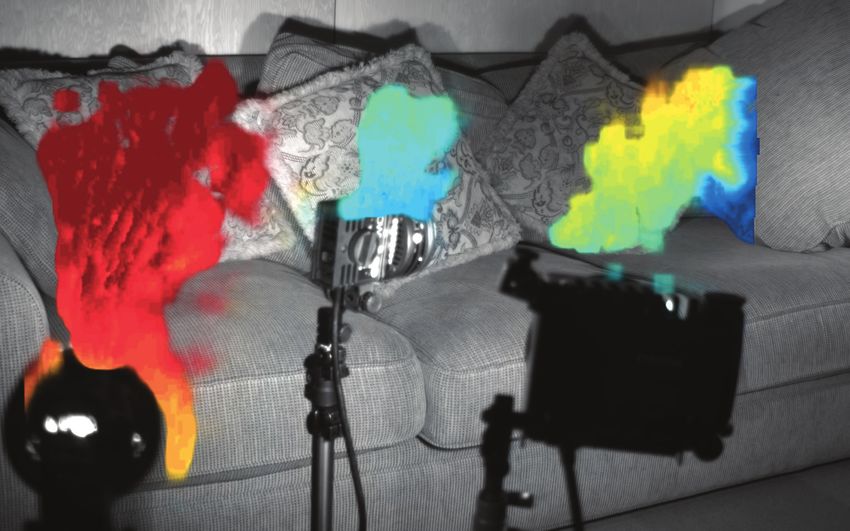
2          Tianfan Xue et al.

                                   Optical                                    Refractive
                                    flow                                        flow

(a) Representative frame (left)              (c) Refraction wiggles (left)                  (e) Velocity of hot air (left)
                                                y

                                                    x
                                   Optical                                     Refractive
                                    flow                                        stereo

                                                                                                                             Pixels

(b) Representative frame (right)             (d) Refraction wiggles (right)                    (f) Disparity of hot air

Fig. 1. Measuring the velocity and depth of imperceptible candle plumes from standard
videos. The heat rising from two burning candles (a, b) cause small distortions of the background
due to light rays refracting as they travel from the background to the camera passing through
the hot air. Methods such as synthetic Schlieren imaging (c, d) are able to visualize those small
disturbances and reveal the heat plume, but are unable to measure its actual motion. We show that,
under reasonable conditions, the refraction patterns (observed motions) move coherently with the
refracting fluid, allowing to accurately measure the 2D motion of the flow from a monocular
video (e), and the depth of the flow from a stereo sequence (f). The full sequence and results are
available in the supplementary material.

However, wiggles are related to the fluid motion in nontrivial ways, and have to be
processed by appropriate algorithms.
    More specifically, measuring refractive flow from video poses two main challenges.
First, since the air or fluid elements are transparent, they cannot be observed directly
by a camera, and the position of intensity texture features is not directly related to the
3D position of the fluid elements. We therefore cannot apply standard motion analysis
and 3D reconstruction techniques directly to the intensity measurements. Our main
observation in this paper is that such techniques are still applicable, but in a different
feature space. Specifically, while intensity features result from a background layer
and their location is not directly related to the fluid layer, motion features (wiggles)
correspond to the 3D positions and motion of points on the transparent fluid surface. The
movement of those wiggles between consecutive frames (i.e. the motion of the observed
motions) is an indicator of the motion of the transparent fluid, and the disparity of these
motion features between viewpoints is a good cue for the depth of the fluid surface.
    Following this observation, we derive algorithms for the following two tasks: 1)
tracking the movement of refractive fluids in a single video, and 2) recovering the 3D
position of points on the fluid surface from stereo sequences. Both these algorithms are
based on the refractive constancy assumption (analogous to the brightness constancy as-
sumption of ordinary motion analysis): that intensity variations over time (the wiggles)
are explained by the motion of a constant, non-uniform refractive field. This distortion
is measured by computing the wiggle features in an input video, and then using those
features to estimate the motion and depth of the fluid, by matching them across frames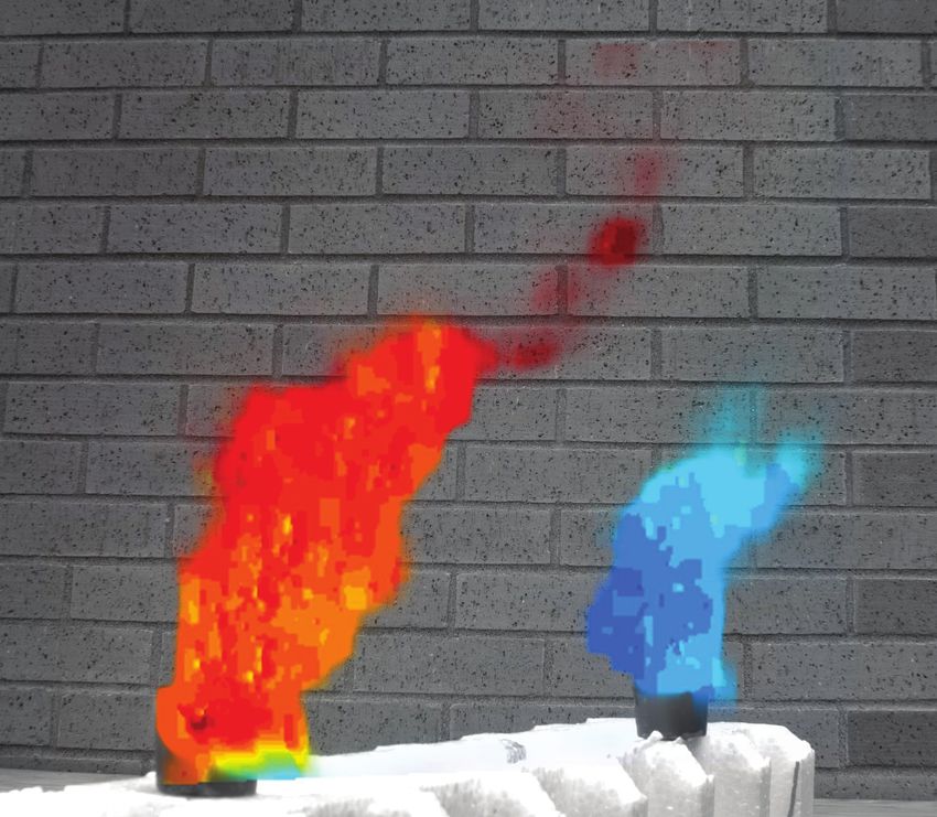
Refraction Wiggles for Measuring Fluid Depth and Velocity from Video      3

and viewpoints. In this paper, we focus on estimating the fluid motion and depth from
stationary cameras, assuming a single, thin refractive layer between the camera and the
background.
    The second challenge in measuring refractive flow from video is that the distortion
of the background caused by the refraction is typically very small (on the order of
0.1 pixels) and therefore hard to detect. The motion features have to be extracted
carefully to overcome inherent noise in the video, and to properly deal with regions
in the background that are not sufficiently textured, in which the extracted motions are
less reliable. To address these issues, we develop probabilistic refractive flow and stereo
algorithms that maintain estimates of the uncertainty in the optical flow, the refractive
flow, and the fluid depth.
    The proposed algorithms have several advantages over previous work: (1) a simple
setup that can be used outdoors or indoors, (2) they can be used to visualize and measure
air flow and 3D location directly from regular videos, and (3) they maintain estimates
of uncertainty. To our knowledge, we are the first to provide a complete pipeline that
measures the motions and reconstructs the 3D location of refractive flow directly from
videos taken in natural settings.
    All the videos and results presented in this paper, together with additional supple-
mentary material, are available on: http://people.csail.mit.edu/tfxue/proj/fluidflow/.

2   Related Work
Techniques to visualize and measure fluid flow can be divided into two categories: those
that introduce tracers (dye, smoke or particles) into the fluid, and those that detect the
refraction of light rays through the fluid, where variations in index of refraction serve
as tracers.
    In tracer-based methods, the fluid motion is measured by tracking particles intro-
duced into the fluid, a technique called particle image velocimetry (PIV). Tradition-
al PIV algorithms are based on correlating the particles between image patches [1].
Recently, optical flow algorithms were used with PIV images [19, 20], and different
regularization terms were proposed to adapt the optical flow methods to track fluids
rather than solid objects [13].
    In tracer-free methods, Schlieren photography is a technique to visualize fluid flow
that exploits changes in the refractive index of a fluid. It works by using a carefully
aligned optical setup to amplify deflections of light rays due to refraction [21, 22, 24,
25]. To measure the velocity of the fluid, researchers have proposed Schlieren PIV [14,
5], in which the motion of a fluid is recovered by tracking vortices in Schlieren pho-
tographs using PIV correlation techniques. These methods still require the optical setup
for Schlieren photography, which can be expensive and hard to deploy outside a lab.
    The initial stage of our approach is most similar to a technique called Background
Oriented Schlieren (BOS, a.k.a Synthetic Schlieren) [6, 8, 10, 12, 15, 18]. The optical
setup in Schlieren photography is replaced by optical flow calculations on a video
of a fluid in front of an in-focus textured background. The refraction due to the fluid
motion is recovered by computing optical flow between each frame of the video and an
undistorted reference frame. Most previous BOS techniques focus on visualizing, not
measuring, the fluid flow, and produce visualizations of the flow similar to the results
shown in Fig. 1(c,d). Atcheson et al. use BOS tomography to recover the volumetric 3D
4       Tianfan Xue et al.

shape of air flow [6]. However, their technique requires a camera array that covers 180◦
of the air flow of the interest, making the whole system difficult to use outdoors. To the
best of our knowledge, ours is the simplest camera-based system–only requiring stereo
video–that can measure the motion and 3D location of air flow.
     While artificial backgrounds are often used when performing BOS [6], Hargather et
al. [12] showed that natural backgrounds, such as a forest, are sufficiently textured for
BOS, allowing for the visualization of large-scale air flows around planes and boats. To
address the fact that the background must be in focus, Wetzstein et al. [28] introduced
light field BOS imaging in which the textured background is replaced by a light field
probe. However, this comes at the cost of having to build a light field probe as large as
the flow of interest.
     Another limitation of the aforementioned BOS algorithms is that they require a
reference frame, which has no air flow in front of it. To avoid having to capture such
a reference frame, Raffel et al. proposed background-oriented stereoscopic Schlieren
(BOSS) [17] , where images captured by one camera serve as reference frames for the
other camera. It is important to note that BOSS uses stereo setup for a different purpose
than our proposed refractive stereo algorithm: the acquisition of a background image,
not depth. BOSS uses stereo to achieve a reference-frame-free capture while we use it
for depth recovery. Moreover, an important weakness of all of these BOS algorithms
is that they require a background that has a strong texture. While texture also helps
our algorithms, the probabilistic framework we propose also allows for more general
backgrounds.
     Complementary to the visualization of BOS, several methods have been developed
to recover quantitative information about a scene from refraction. Several authors have
shown that it is possible to recover the shape of the surface of an air-water interface by
filming a textured background underneath it [9, 16, 30]. Alterman et al. [4] proposed to
recover refraction location and strength from multiple cameras using tomography. Tian
et al. [27] showed that atmospheric turbulence provides a depth cue as larger deflections
due to refraction typically correspond to greater depths. Wetzstein et al. [29] proposed
to recover the shape of a refractive solid object from light field distortions. Alterman
et al. [2, 3] showed that it is possible to locate a moving object through refractive
atmospheric turbulence or a water interface.

3   Refraction Wiggles and Refractive Constancy
Gradients in the refractive properties of air (such as temperature and shape) introduce
visual distortions of the background, and changes in the refractive properties over time
show up as minute motions in videos. In general, several factors may introduce such
changes in refractive properties. For example, the refractive object may be stationary
but change in shape or temperature. In this paper, however, we attribute those changes to
non-uniform refractive flow elements moving over some short time interval [t, t + Δt].
We assume that for a small enough Δt, a refractive object maintains its shape and
temperature, such that the observed motions in the video are caused mostly by the
motion of the object (and the object having a non-uniform surface, thus introducing
variation in the refractive layer). While this is an assumption, we found it to hold well
in practice as long as the video frame-rate is high enough, depending on the velocity of
the flow being captured (more details in the experimental section below). In this section,
Refraction Wiggles for Measuring Fluid Depth and Velocity from Video 5
ݔ௧ᇱᇱమ Background ݔ௧ᇱᇱభ
࢚ ܍ܕܑ܂ ܜ ܗܜ + ઢܜ ࢚ ܍ܕܑ܂ ܜ ܗܜ + ઢߙ ܜ௧ᇱభା௧
ߙ௧ᇱభ
ݖԢԢ ߙ௧ᇱమା௧ ߙ௧ᇱమ
ݔ௧ᇱమା௧ ݔ௧ᇱమ ݔ௧ᇱభା௧ ݔ௧ᇱభ
ݖԢ Wiggle ݐ(ݒଶ ) Wiggle ݐ(ݒଵ )
ݔ௧మା௧ ݔ௧మ ݔ௧భା௧ ݔ௧భ Image plane
ߙ௧భ
ߙ௧మ
ݖ ߙ௧మା௧ ߙ௧భା௧
Center of projection
(a) Refractive flow
ᇱᇱ ᇱᇱ
ݔ௧,ଶ ݔ௧,ଵ Background
ᇱ ᇱ
ߙ௧ା௧,ଵ ᇱ
ߙ௧,ଶ ߙ௧,ଵ
ݖԢԢ ᇱ
ܜ ܍ܕܑ܂ + ઢܜ ߙ௧ା௧,ଶ ࢚ ܍ܕܑ܂
ᇱ ᇱ
ᇱ ᇱ ݔ௧,ଵ (= ݔ௧,ଶ )
ݔ௧ା௧,ଵ (= ݔ௧ା௧,ଶ )
ݖԢ
Wiggle ݒଵ (ݐଵ ) Wiggle ݒଶ (ݐଵ )
ݔ௧ା௧,ଵ ݔ௧,ଵ ݔ௧ା௧,ଶ ݔ௧,ଶ Image plane 2
Image plane 1
ߙ௧,ଵ ߙ௧ା௧,ଶ
ݖ ߙ௧ା௧,ଵ ߙ௧,ଶ
ଵ Center of projection 1 ଶ Center of projection 2
(b) Refractive stereo
Fig. 2. Refractive distortions (wiggles) in a single view (a) and multiple views (b). A single,
thin refractive layer is moving between one or more video cameras and a background. As the
refractive fluid moves between time ti (solid lines) and time ti +Δt (dashed lines), changes in the
refractive patterns move points on the background (shown in blue and red) to different positions
on the image plane, generating the observed “wiggles” (red and blue arrows). The direction of
the wiggles on the image plane can be arbitrary, but they are consistent over short time durations
and between close viewpoints as the fluid moves (see text). By tracking the wiggles over time we
can recover the projected 2D fluid motion (a), and by stereo-fusing the wiggles between different
views, we can recover the fluid’s depth (b). Note: as discussed in the text, wiggle constancy holds
if the refraction, the motion of the object and the baseline between the cameras are small. In these
illustrations we exaggerated all these quantities for clarity.
we establish the relation between those observed motions in one or more cameras and
the motion and depth of refractive fluids in a visual scene.
To understand the basic setup, consider Fig. 2. A video camera, or multiple video
cameras, are observing a static background through a refractive fluid layer (such as hot
air). In this paper, we assume that the cameras are stationary, and that a single, thin
and moving refractive layer exists between the camera and the background. We use the
notation xt,j for points on the j’th camera sensor plane at time t, xt,j for points on the
(locally planar) fluid, and xt,j for background points, where t denotes the time index.
The depths of these planes are denoted by z, z , z , respectively. We denote the camera
centers by oj , and denote by αt,j , αt,j the angles between the optical axis to the ray
6       Tianfan Xue et al.

from the j’th camera center to points on the image plane and background, respectively.
For brevity, we will omit the subscript j in the case of a single camera.
    Now consider the stereo setup in Fig. 2(b). An undistorted ray from the camera
center oj to points xt,j , xt,j on the j’th camera plane has angle (assuming small αt,j ,
such that tan αt,j ≈ αt,j )
                         αt,j = (xt,j − oj )/z = (xt,j − oj )/z  .                      (1)

     This ray is distorted as it passes through the fluid, and transfers into angle αt,j . The
exact distortion is determined by Snell’s law. As is common in the optics literature,
if the difference between the incident and refraction angles is small, we can use first
order paraxial approximations, which imply that Snell’s refraction law is effectively an
additive constant,

                                     αt,j  ≈ αt,j + Δαt ,                                  (2)
where the angle difference Δαt depends only on the local geometric and refractive
properties of the fluid around the intersection point xt , and is independent of the in-

coming ray direction αt,j , and in particular independent of the location of the observing
camera oj . The distorted ray then hits the background surface at the point
                     xt,j = xt,j + ζ · αt,j

                                               = xt,j + ζ (αt,j + Δαt )                  (3)
where ζ = z  − z  is the distance between the fluid object and the background.
    At a successive time step t + Δt the fluid moves (dashed gray blob in Fig. 2(b)). We
assume this motion introduces an observed motion of the projection of the background
point xt,j on the image plane, from point xt,j to point xt+Δt,j . We call that motion a
“refraction wiggle”, or “wiggle” for short. The geometry of the fluid can be complex
and predicting the exact path of the light ray mathematically is not straightforward.
Nevertheless, We define as xt+Δt,j the point at which a ray connecting xt,j to the
camera center oj intersects and refracts at the fluid layer.
    Let us now fix a point x̄t = xt,j on the fluid surface, and refer to the image xt,j of
that same physical point in all cameras. The rays from each camera to that point have

different angles αt,j  , and as a result they intersect the background layer at different

points xt,j . Thus, the texture intensity observed by each camera at the points xt,j can
be arbitrarily different. Therefore, we cannot match intensities between the cameras
if we wish to match features on the fluid layer and recover their depth. However, we
observe that the wiggles correspond to features on the fluid layer rather than on the
background, which allows us to stereo-fuse them to estimate the fluid depth. For this
we need to show that despite the fact that, without loss of generality, xt,1 = xt,2 , the
two points are refracted at time t + Δt via the same fluid point xt+Δt,1 = xt+Δt,2 . To
see that, we use Eq. (3) to express
             xt+Δt,j − xt,j = −ζ(αt+Δt,j − αt,j ) − ζ(Δαt+Δt − Δαt ),                   (4)
and from Eq. (1), we have
                         αt+Δt,j − αt,j = (xt+Δt,j − xt,j )/z  .                       (5)
Plugging Eq. (5) in Eq. (4) we thus have
                         xt+Δt,j − xt,j = c · (Δαt+Δt − Δαt ),                          (6)
Refraction Wiggles for Measuring Fluid Depth and Velocity from Video        7

where c = −(z  − z  )z  /z  . Therefore, since the terms on the RHS of Eq. (6) are
all camera-independent (under our setup and assumptions), if xt,1 = xt,2 = x̄t , we
conclude that xt+Δt,1 = xt+Δt,2 and the wiggles in both cameras are equal.
    This refraction constancy can be shown similarly for the monocular case (Fig. 2(a)).
That is, if the fluid object is moving at constant velocity over a short spatio-temporal
window, then the observed refraction wiggles move coherently with the fluid object
between consecutive frames. This stands in contrast to the fact that the observed motions
themselves (the wiggles) are unrelated to the actual fluid motion, and in fact can point in
opposite directions (Fig. 1, Fig. 4). We refer the interested reader to our supplementary
material for the derivation, as well as for a more detailed version of the derivation we
gave here. Also note that in Eq. (1) and Eq. (3) we assumed the viewing angle α is small
to simplify the derivation, however refraction constancy is not restricted by the viewing
angle (not to be confused with Δα, which does need to be small). In the supplementary
material we give the derivation without making this assumption.
    The practical implication of the observations we made in this section is that if
we wish to match the projection of a point on the fluid object across frames or
viewpoints, we can match the observed wiggle features. That is, while the position
of intensity texture features is unrelated to the fluid 3D structures, the position of wiggle
features respect features on the fluid surface, and can serve as an input feature for optical
flow and stereo matching algorithms. In the following sections we will use this to derive
optical flow and stereo algorithms for tracking and localizing refractive fluids.

4   Refractive Flow
The goal of fluid motion estimation is to recover the projected 2D velocity, u(x, y, t),
of a refractive fluid object from an observed image sequence, I(x, y, t) (Fig. 2(a)).
As discussed in the previous section, the wiggle features v(x, y, t), not the image
intensities I(x, y, t), move with the refractive object. Thus, there are two steps in es-
timating the fluid’s motion: 1) computing the wiggle features v(x, y, t) from an input
image sequence I(x, y, t), and 2) estimating the fluid motion u(x, y, t) from the wiggle
features v(x, y, t). We will now discuss each of these steps in turn.

Computing wiggle features. We use optical flow to compute the wiggles v(x, y, t) from
an input image sequence. Recall the brightness constancy assumption in optical flow is
that any changes in pixel intensities, I, are assumed to be caused by a translation v =
(vx , vy ) over spatial horizontal or vertical positions, x and y, of the image intensities,
where vx and vy are the x and y components of the velocity, respectively. That is,

                        I(x, y, t + dt) = I(x − vx dt, y − vy dt, t).                   (7)

Based on this brightness constancy equation, a traditional way to calculate the motion
vector v is to minimize the following optical flow equation [7]:
                                                 2
                                ∂I   ∂I      ∂I         ∂v 2  ∂v 2
         ṽ = arg min
                            α 1  vx +    vy +
                                                     + α2
                                                                 +     ,               (8)
                   u
                        x
                                  ∂x   ∂y      ∂t          ∂x     ∂y

where α1 and α2 are weights for the data and smoothness terms, respectively.
8           Tianfan Xue et al.

    (a) Source
     (candle)

                    (b) Wiggles, visualized in two ways   (c) Refractive flow (d) Prob. refractive flow
Fig. 3. Example result of our refractive flow algorithm (single view) on a sequence of burning
candles. Wiggle features (b) are extracted from the input video (a). Notice how the directions of
the wiggles (observed motions) are arbitrary and inconsistent with the air flow direction (the right
visualization in (b) uses the same wiggle color coding as in Fig. 1). (c) and (d) show refractive
flows calculated by two algorithms, refractive flow and probabilistic refractive flow, respectively.

Estimating fluid motion. Let ux and uy be the x and y components of the fluid’s veloc-
ity as seen in the image. Following Section 3, we thus define the refractive constancy
equation for a single view sequence as
                           v(x, y, t + Δt) = v(x − ux Δt, y − uy Δt, t).                           (9)
 Notice that refractive constancy has the exact same form as brightness constancy
(Eq. 7), except that the features are the wiggles, v, rather than the image intensities,
I. This implies that running an optical flow algorithm on the wiggle features v (i.e. the
motion of the motion features), will yield the fluid motion u.
    Formally, we calculate the fluid motion u by minimizing the following equation:
                                                          2
                                  ∂ ṽ     ∂ ṽ     ∂ ṽ           ∂u 2  ∂u 2
            ũ = arg min       β1       u +
                                   ∂x x ∂y y     u +        + β         +
                                                                               ∂y  .            (10)
                                                      ∂t             ∂x
                                                                  2
                      u
                           x

  This is similar to the Horn-Schunck optical flow formulation, except that we use
L2 -norm for regularization, as opposed to robust penalty functions such as L1 -norm
traditionally used by optical flow methods. This is because fluid objects, especially hot
air or gas, do not have clear and sharp boundaries like solid objects. We use a multi-scale
iterative algorithm to solve Eq. 10, as is common in the optical flow literature.
     Fig. 3 demonstrates a result of this refractive flow algorithm, when applied to a
video of burning candles. First, wiggle features (Fig. 3(b)) are extracted from the input
video (Fig. 3(a)). Since wiggle features move coherently with the air flow, the algorithm
correctly estimates the motion of the thermal plume rising from the candle. Notice that
the observed motions (wiggles) have arbitrary directions, yet the estimated refractive
flow is much more coherent.
     Such processing is very sensitive to noise, however, as can be seen in Fig. 3(b) (the
noise is more obvious in an enlarged image). The problem is even more severe for less
textured backgrounds. This motivates the probabilistic formulation, which we will now
describe.

4.1      Probabilistic Refractive Flow
We seek to estimate both the refractive flow, and its uncertainty. Consider a background
that is smooth in the x direction and textured in the y direction. Due to the aperture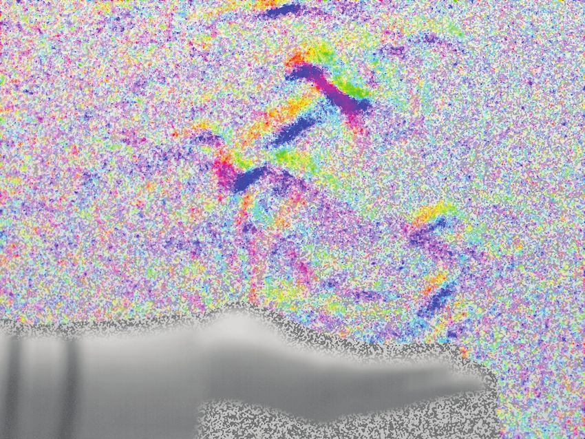
Refraction Wiggles for Measuring Fluid Depth and Velocity from Video       9

problem [11], the flow in the x direction may be dominated by noise, while the opti-
cal flow in the y direction can be clean. Knowing the uncertainty in the flow allows
uncertain estimates to be down-weighted, increasing the robustness of the algorithm.
    To find the variance of the optical flow, let us reformulate Eq. (8) as a posterior
distribution:
                                                 2
                                 ∂I   ∂I      ∂I         ∂v 2       ∂v 2
    P (v|I) = exp −
                             α 1  vx +    vy +
                                                      + α2
                                                                   + α2      .        (11)
                         x
                                   ∂x   ∂y      ∂t          ∂x          ∂y

 Here, P (v|I) is a Gaussian distribution, and the mean of P (v|I) is equal to the
solution of the original optical flow equation (8). With this formulation, we can also
calculate the variance of the optical flow (the wiggle features). Please refer to the
supplementary material for the detailed calculation. Let ṽ and Σv be the mean and
covariance, respectively, of the wiggle features computed from Eq. (11).
    Then, with the variance of the wiggle features, we can reweight the fluid flow
equation as follows:
                                                2
                      ∂ ṽ      ∂ ṽ      ∂ ṽ         ∂u 2  ∂u 2
ũ = arg min
                   β1       ux +      uy +
                                                    + β2
                                                                +       + β3 u2 , (12)
         u
               x
                        ∂x        ∂y        ∂t Σv         ∂x     ∂y

 where  x2Σ    = x Σ −1 x is the squared Mahalanobis distance. In this formulation,
the data term is reweighted by the variance of the optical flow to robustly estimate the
fluid motion: wiggle features with less certainty, such as motions measured in regions
of low-contrast, or of flat or one-dimensional structure, will have lower weight in the
fluid flow equation. To increase the robustness, we also penalize the magnitude of u
to avoid estimating spurious large flows. Including the uncertainty information leads to
more accurate estimation of the fluid motion, as shown in Fig. 3(d).
    In practice, calculating the covariance matrix precisely for each pixel is compu-
tationally intractable, as we need to compute the marginal probability distribution for
each optical flow vector. To avoid this calculation, we concatenate all the optical flow
vectors into a single vector and compute its covariance. See the supplementary material
for the details. Also, notice that the fluid flow equation (12) still has a quadratic form,
so we can model the posterior distribution of the fluid flow u as a Gaussian distribution,
and compute its variance. This variance serves as a confidence measure in the estimated
fluid motion.

5   Refractive Stereo
The goal of fluid depth estimation is to recover the depth z  (x, y) of a refractive fluid ob-
ject from a stereo sequence IL (x, y, t) and IR (x, y, t) (Fig. 2(b)). Following Section 3,
we can find the depth of the fluid object by stereo-matching the refraction wiggles from
the left and right views. Therefore, we first use the algorithm discussed in the previous
section to calculate the mean and variance of the optical flows in the left and right views,
vL ∼ N (ṽL , ΣL ) and vR ∼ N (ṽR , ΣR ), respectively. We then use a discrete Markov
Random Field (MRF), commonly used in the stereo literature [23], to regularize the
depth estimates.
    Formally, let xL and xR be the projection of a point on the fluid object onto the left
and right image plane, respectively, and define disparity as d = xL − xR . We first solve
the disparity map by minimizing the objective function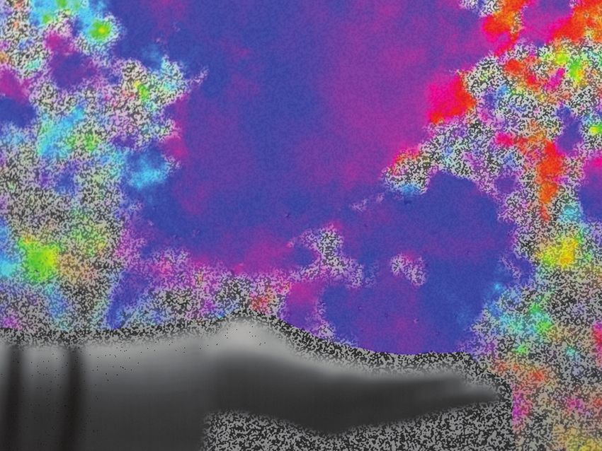
10         Tianfan Xue et al.

                                                              ∂d 2  ∂d 2
      d̃ = min         f (vR (x, y), vL (x + d(x, y), y)) + α
                                                               ∂x  +  ∂y  ,       (13)
             d
                 x,y

where f (vR , vL ) is the data term based on the observed wiggles vR and vL , and
the last two terms regularize the disparity field. We found that using the L2 -norm for
regularization generates better results overall, better explaining the fuzzy boundaries of
fluid refractive objects (similar to what we observed for estimating the optical flow in
Section 4).
    As with the refractive flow, we weigh the data term by the variance of the optical
flow to make the depth estimation robust to points in a scene where the extracted
wiggles are not as reliable. To achieve this, we define the data term, f (vR , vL ), as
the log of the covariance between the two optical flows from the left and right views,
                                             1                 1
      f (ṽR , ṽL ) = log cov(vR , vL ) =     log |ΣL + ΣR | + vR − vL 2ΣL +ΣR ,   (14)
                                             2                 2
where vR − vL 2ΣL +ΣR = (vR − vL ) (ΣL + ΣR )−1 (vR − vL ). This data term will
assign a higher penalty to inconsistencies in the wiggle matching where the wiggles are
more reliable, and a lower penalty where the wiggles are less reliable (typically where
the background is less textured and the optical flow is noisy). The choice of the log of
the covariance as the data term is not arbitrary. It is the log of the conditional marginal
distribution of vL and vR , given that vL and vR match. See the supplementary material
for a detailed derivation.
    With calibrated cameras, we can then compute the depth map, z  (x, y), from the
disparity map, d(x, y).

6      Experiments
We show several examples of measuring and localizing hot air radiating from several
heat sources, such as people, fans, and heating vents. Please refer to the supplemen-
tary materials for the full sequences and results.
    All the videos were recorded in raw format to avoid compression artifacts. To deal
with small camera motions or background motions, we subtracted the mean flow for
each frame from the optical flow result. For each sequence we captured, we first applied
a temporal Gaussian blur to the input sequence to increase SNR. For fast-moving flow,
we recorded high-speed videos using a Phantom v10 high-speed camera. In some of
the indoor high-speed sequences that required additional lighting, we used a temporal
band-stop filter to remove intensity variations from the lighting due to AC power.

6.1     Refractive Flow
Qualitative Results. In Fig. 4 we show several results of refractive flow analysis from
a single camera.
    We first tested our algorithm in a controlled setting, using a textured background.
In hand, we took a 30fps video of a person’s hand after he held a cup of hot water. The
algorithm was able to recover heat radiating upward from the hand. In hairdryers, we
took a 1000fps high-speed video of two hairdryers placed in opposite directions (the
Representative frame Refraction Wiggles for Measuring Fluid Depth and Velocity from Video 11
hand hairdryer kettle vents
Refractive flow (var) Refractive flow (mean) Optical flow (mean)
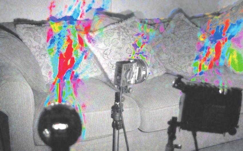
Fig. 4. Refractive flow results. First row: sample frames from the input videos. Second row:
the mean of the optical flow for the same representative frames (using the colormap shown in
Fig. 1), overlayed on the input images. Third row: the mean of the refractive flow, weighted
by the variance. Fourth row: the variance of the estimated refractive flow (the square root of the
determinant of the covariance matrix for each pixel). For this visualization, variance values above
0.03 were clipped. The full videos are available in the accompanying material.
two dark shapes in the top left and bottom right are the front ends of the hairdryers),
and our algorithm detected two opposite streams of hot air flows.
kettle and vents demonstrate the result on videos with more natural backgrounds.
In vents (700fps), the background is very challenging for traditional Background Ori-
ented Schlieren algorithms (BOS), as some parts of the background are very smooth or
contain edges in one direction, such as the sky, the top of the dome, and the boundary
of the buildings or chimneys. BOS algorithms rely on the motion calculated from input
videos, similar to the wiggle features shown in the second row of Fig. 4, which is very
noisy due to the insufficiently textured background. In contrast, the fluid flow (third
row of Fig. 4) clearly shows several flows of hot air coming out from heating vents.
By modeling the variance of wiggles in the probabilistic refractive flow (bottom row of
Fig. 4), most of noise in the motion is suppressed.
Quantitative Evaluation. To quantitatively evaluate the fluid velocity recovered by the
proposed algorithm, we tested it on simulated sequences with precise ground truth.
We generated a set of realistic simulations of dynamic refracting fluid using Stable12 Tianfan Xue et al.
50
Angular Error (degree)
40
30
Tex 1
20 Tex 2
Tex 3
10
5 10 20 40 80 160 320 640
Tempature Difference
(a) Simulated fluid (b) Grounth truth motion (c) Refractive flow result (d) Backgrounds (e) Flow estimation error
Fig. 5. Quantitative evaluation of refractive flow using synthetic sequences. Simulated fluid
density (a) and velocity field (b) were generated by Stable Fluids [26], a physics-based fluid flow
simulation technique, and rendered on top of three different textures (d). The recovered velocity
field from one of the simulations in which the fluid was at 320◦ Celsius (c) is similar to the ground
truth velocity field (b). Quantitative evaluation is given in (e). As expected, larger temperature-
related index of refraction differences between the fluid and the background give better flow
estimates. The error also increases for backgrounds that do not contain much texture.
Hairdryer
By By
Ruler Algorithm Velometer
x1 0.8 0.0
x2 1.4 0.3
(b) Representative frame
x3 3.2 1.4
x4 12.0 13.8
(d) velocities (in m/s)
for the points in (c)
Velometer
(a) Setup (c) Estimated flow velocity (in m/s)
Fig. 6. Quantitative evaluation of refractive flow using a controlled experiment. (a) The
experiment setup. (b) A representative frame from the captured video. (c) The mean velocity
of the hot air blown by the hairdryer, as computed by our algorithm, in m/s. (d) Numerical
comparison of our estimated velocities with velocities measured using a velometer, for the four
points marked x1 − x4 in (c).
Fluids [26], a physics-based fluid flow simulation technique, resulting in fluid densities
and (2D) ground truth velocities at each pixel over time (Fig. 5(a-b)). We then used
the simulated densities to render refraction patterns over several types of background
textures with varying spatial smoothness (Fig. 5(d)). To render realistic refractions, we
assumed the simulated flow is at a constant distance between the camera and back-
ground, with thickness depending linearly on its density (given by the simulation). For
a given scene temperature (we used 20◦ Celsius) and a temperature of the fluid, we can
compute exactly the amount of refraction at every point in the image. We then apply our
algorithm to the refraction sequences. The angular error of the recovered fluid motion
at different temperature is shown in (e). All the sequences and results are available in
the supplemental material.
To further demonstrate that the magnitude of the motion computed by the refractive
flow algorithm is correct, we also performed a controlled experiment shown in Fig. 6.
We use a velocimeter to measure the velocity of hot air blown from a hairdryer, and
compare it with the velocities extracted by the algorithm. To convert the velocity on the
image plane to the velocity in the real world, we set the hairdryer parallel to the imagingRefraction Wiggles for Measuring Fluid Depth and Velocity from Video 13
plane and put a ruler on the same plane of the hairdryer. We measured the velocity of
the flow at four different locations as shown in Fig. 6(c). Although our estimated flow
does not match the velocimeter flow exactly, it is highly correlated, and we believe the
agreement is accurate to within the experimental uncertainties.
6.2 Refractive Stereo
Qualitative Results. We captured several stereo sequences using our own stereo rig,
comprised of two Point Grey Grasshopper 3 cameras recording at 50fps. The two
cameras are synchronized via Genlock and global shutter is used to avoid temporal
misalignment. All videos were captured in 16-bit grayscale.
Several results are shown in Fig. 7. The third row in Fig. 7 shows the disparity map
of air flow as estimated by our refractive stereo algorithm, and the forth row shows
a 3D reconstruction of the scene according to the estimated depths of the solid and
refractive objects. For the 3D reconstructions, we first used a standard stereo method
to reconstruct the (solid) objects and the background, and then rendered fluid pixels
according to their depth as estimated by our refractive stereo algorithm, colored by their
disparities (and weighted by the confidence of the disparity). In candle, two plumes
of hot airs at different depth are recovered. In lamps, three lights were positioned at
different distances from the camera: the left one was the closest to the camera and the
middle one was the furthest. The disparities of three plumes recovered by the algorithm
match the locations of the lights. In monitor, the algorithm recovers the location of hot
air radiating from the center top of a monitor. We intentionally tilted the monitor such
that its right side was closer to the camera to introduce variation in the depth of the air
flow. The algorithm successfully detects this gradual change in disparities, as shown in
the right column of Fig. 7.
Quantitative Evaluation. We compared the recovered depths of the refractive fluid
layers with that of the heat sources generating them, as computed using a standard
stereo algorithm (since the depth of the actual heat sources, being solid objects, can be
estimated well using existing stereo techniques). More specifically, we picked a region
on the heat source and picked another region of hot air right above the heat source
(second row in Fig. 7), and compared the average disparities in these two regions. The
recovered depth map of the (refractive) hot air matched well the recovered depth map
of the (solid) heat sources, with an average error of less than a few pixels (bottom row
in Fig. 7). We show more evaluations of our refractive stereo algorithm using synthetic
experiments in the supplementary material.
7 Conclusion
We proposed novel methods for measuring the motion and 3D location of refractive
fluids directly from videos. The algorithms are based on wiggle features, which cor-
responds to the minute distortions of the background caused by changes in refraction
as refractive fluids move. We showed that wiggles are locally constant within short
time spans and across close-by viewpoints. We then used this observation to propose
a refractive flow algorithm that measures the motion of refractive fluids by tracking
wiggle features across frames, and a refractive stereo algorithm that measures the depth14 Tianfan Xue et al.
lamps candle monitor
:LJJOHV OHIW
:LJJOHV ULJKW
'LVSDULWLHV
(YDOXDWLRQ 'UHFRQVWUXFWLRQ
300 170 190
Disparity (pixels)
Disparity (pixels)
Disparity (pixels)
160
280
150 180 6ROLG
260 140
)OXLG
170 6ROLG
130
240 )OXLG
120
160 6ROLG
220 110
)OXLG
100
200 150
0 20 40 60 80 0 50 100 150 0 5 10 15 20
Time (frame) Time (frame) Time (frame)
Fig. 7. Refractive stereo results. First and second rows: representative frames from the input
videos. The observed wiggles are overlayed on the input frames using the same color coding as
in Fig. 1. Third row: the estimated disparity maps (weighted by the confidence of the disparity) of
the fluid object. Forth row: 3D reconstruction of the scene, where standard stereo is used for solid
objects (and the background), and refractive stereo is used for air flows (the depth was scaled
for this visualization). Bottom row: Comparison of our estimated refractive flow disparities, with
the disparities of the (solid) heat sources that generated them as computed with a standard stereo
algorithm, for the points marked as rectangles on the frames in the second row.
of the fluids by matching wiggle features across different views. We further proposed
a probabilistic formulation to improve the robustness of the algorithms by modeling
the variance of the observed wiggle signals. This allows the algorithms to better handle
noise and more natural backgrounds. We demonstrated results on realistic, physics-
based fluid simulations, and recovered flow patterns from controlled and natural monoc-
ular and stereo sequences. These results provide promising evidence that refractive
fluids can be analyzed in natural settings, which can make fluid flow measurement
cheaper and more accessible.Refraction Wiggles for Measuring Fluid Depth and Velocity from Video 15
Acknowledgements We thank the ECCV reviewers for their comments. Tianfan Xue was
supported by Shell International Exploration & Production Inc. and Motion Sensing Wi-Fi Sensor
Networks Co. under Grant No. 6925133. Neal Wadhwa was supported by the NSF Graduate
Research Fellowship Program under Grant No. 1122374. Part of this work was done when
Michael Rubinstein was a student at MIT, supported by the Microsoft Research PhD Fellowship.
We also acknowledge support from ONR MURI grant N00014-09-1-1051.
References
1. Adrian, R.J., Westerweel, J.: Particle image velocimetry. Cambridge University Press (2011)
2. Alterman, M., Schechner, Y.Y., Perona, P., Shamir, J.: Detecting motion through dynamic
refraction. IEEE Trans. Pattern Anal. Mach. Intell. 35(1), 245–251 (2013)
3. Alterman, M., Schechner, Y.Y., Swirski, Y.: Triangulation in random refractive distortions.
In: Computational Photography (ICCP), 2013 IEEE International Conference on. pp. 1–10.
IEEE (2013)
4. Alterman, M., Schechner, Y.Y., Vo, M., G, S.N.: Passive tomography of turbulence strength.
In: Proc. of European Conference on Computer Vision (ECCV). IEEE (2014)
5. Arnaud, E., Mémin, E., Sosa, R., Artana, G.: A fluid motion estimator for schlieren image
velocimetry. In: Proc. of European Conference on Computer Vision (ECCV). pp. 198–210.
IEEE (2006)
6. Atcheson, B., Ihrke, I., Heidrich, W., Tevs, A., Bradley, D., Magnor, M., Seidel, H.P.: Time-
resolved 3D capture of non-stationary gas flows. ACM Trans. Graph. 27(5), 132:1–132:9
(Dec 2008)
7. Baker, S., Scharstein, D., Lewis, J., Roth, S., Black, M., Szeliski, R.: A database and
evaluation methodology for optical flow. International Journal of Computer Vision 92(1),
1–31 (2011)
8. Dalziel, S.B., Hughes, G.O., Sutherland, B.R.: Whole-field density measurements by
synthetic schlieren. Experiments in Fluids 28(4), 322–335 (2000)
9. Ding, Y., Li, F., Ji, Y., Yu, J.: Dynamic fluid surface acquisition using a camera array. In:
Computer Vision (ICCV), 2011 IEEE International Conference on. pp. 2478–2485 (2011)
10. Elsinga, G., van Oudheusden, B., Scarano, F., Watt, D.: Assessment and application
of quantitative schlieren methods: Calibrated color schlieren and background oriented
schlieren. Experiments in Fluids 36(2), 309–325 (2004)
11. Fleet, D., Weiss, Y.: Optical flow estimation. In: Handbook of Mathematical Models in
Computer Vision, pp. 237–257. Springer US (2006)
12. Hargather, M.J., Settles, G.S.: Natural-background-oriented schlieren imaging. Experiments
in Fluids 48(1), 59–68 (2010)
13. Has, P., Herzet, C., Mmin, E., Heitz, D., Mininni, P.D.: Bayesian estimation of turbulent
motion. IEEE Trans. Pattern Anal. Mach. Intell. 35(6), 1343–1356 (June 2013)
14. Jonassen, D.R., Settles, G.S., Tronosky, M.D.: Schlieren “PIV” for turbulent flows. Optics
and Lasers in Engineering 44(3-4), 190–207 (2006)
15. Meier, G.: Computerized background-oriented schlieren. Experiments in Fluids 33(1), 181–
187 (2002)
16. Morris, N.J., Kutulakos, K.N.: Dynamic refraction stereo. In: Computer Vision (ICCV), 2005
IEEE International Conference on. vol. 2, pp. 1573–1580 (2005)
17. Raffel, M., Tung, C., Richard, H., Yu, Y., Meier, G.: Background oriented stereoscopic
schlieren (BOSS) for full scale helicopter vortex characterization. In: Proc. of International
Symposium on Flow Visualization (2000)
18. Richard, H., Raffel, M.: Principle and applications of the background oriented schlieren
(BOS) method. Measurement Science and Technology 12(9), 1576 (2001)16 Tianfan Xue et al.
19. Ruhnau, P., Kohlberger, T., Schnrr, C., Nobach, H.: Variational optical flow estimation for
particle image velocimetry. Experiments in Fluids 38(1), 21–32 (2005)
20. Ruhnau, P., Schnrr, C.: Optical stokes flow estimation: an imaging-based control approach.
Experiments in Fluids 42(1), 61–78 (2007)
21. Ruhnau, P., Stahl, A., Schnrr, C.: On-line variational estimation of dynamical fluid flows
with physics-based spatio-temporal regularization. In: Pattern Recognition, Lecture Notes in
Computer Science, vol. 4174, pp. 444–454. Springer Berlin Heidelberg (2006)
22. Schardin, H.: Die schlierenverfahren und ihre anwendungen. In: Ergebnisse der exakten
Naturwissenschaften, pp. 303–439. Springer (1942)
23. Scharstein, D., Szeliski, R.: A taxonomy and evaluation of dense two-frame stereo
correspondence algorithms. International Journal of Computer Vision 47(1-3), 7–42 (2002)
24. Settles, G.S.: Schlieren and shadowgraph techniques: visualizing phenomena in transparent
media, vol. 2. Springer Berlin (2001)
25. Settles, G.S.: The penn state full-scale schlieren system. In: Proc. of International
Symposium on Flow Visualization (2004)
26. Stam, J.: Stable fluids. In: Proceedings of the 26th Annual Conference on Computer Graphics
and Interactive Techniques. pp. 121–128. SIGGRAPH ’99, ACM Press/Addison-Wesley
Publishing Co., New York, NY, USA (1999)
27. Tian, Y., Narasimhan, S., Vannevel, A.: Depth from optical turbulence. In: Computer Vision
and Pattern Recognition (CVPR), 2012 IEEE Conference on. pp. 246–253. IEEE (June 2012)
28. Wetzstein, G., Raskar, R., Heidrich, W.: Hand-held schlieren photography with light field
probes. In: Computational Photography (ICCP), 2011 IEEE International Conference on.
pp. 1–8 (April 2011)
29. Wetzstein, G., Roodnick, D., Heidrich, W., Raskar, R.: Refractive shape from light field
distortion. In: Computer Vision (ICCV), 2011 IEEE International Conference on. pp. 1180–
1186 (2011)
30. Ye, J., Ji, Y., Li, F., Yu, J.: Angular domain reconstruction of dynamic 3d fluid surfaces. In:
Computer Vision and Pattern Recognition (CVPR), 2012 IEEE Conference on. pp. 310–317
(2012)You can also read