Non closed acoustic cloaking devices enabled by sequential step linear coordinate transformations - Nature
←
→
Page content transcription
If your browser does not render page correctly, please read the page content below
www.nature.com/scientificreports
OPEN Non‑closed acoustic cloaking
devices enabled by sequential‑step
linear coordinate transformations
Zahra Basiri1,4, Mohammad Hosein Fakheri1,4, Ali Abdolali1,4* & Chen Shen2,3,4
Hitherto acoustic cloaking devices, which conceal objects externally, depend on objects’
characteristics. Despite previous works, we design cloaking devices placed adjacent to an arbitrary
object and make it invisible without the need to make it enclosed. Applying sequential linear
coordinate transformations leads to a non-closed acoustic cloak with homogeneous materials,
creating an open invisible region. Firstly, we propose to design a non-closed carpet cloak to conceal
objects on a reflecting plane. Numerical simulations verify the cloaking effect, which is completely
independent of the geometry and material properties of the hidden object. Moreover, we extend this
idea to achieve a directional acoustic cloak with homogeneous materials that can render arbitrary
objects in free space invisible to incident radiation. To demonstrate the feasibility of the realization,
a non-resonant meta-atom is utilized which dramatically facilitated the physical realization of our
design. Due to the simple acoustic constitutive parameters of the presented structures, this work
paves the way toward realization of non-closed acoustic devices, which could find applications in
airborne sound manipulation and underwater demands.
Invisibility cloak is one of the most attractive research topics due to its exotic properties in deflecting the waves
around objects. A powerful approach to achieve invisibility devices is the coordinate transformation method
firstly utilized by Pendry et al. for the design of ideal electromagnetic (EM) c loak1. Not long after, Cummer and
Schurig presented a two-dimensional (2D) acoustic cloak by illustrating the analogy between 2D time harmonic
Maxwell equations and acoustic wave e quations2. Later, a similar coordinate transformation method was further
extended to design of 3D acoustic cloaks by Chen and Chan3. The same relations through the acoustic scattering
theory were also derived i n4 by Cummer et al. Due to the potential applications of cloaking in a variety of both
acoustics and electromagnetics scenarios, numerous schemes have been devoted to theoretical development
and fabrication of cloaking devices5–10. The major difficulty in ideal cloak implementation is the requirement of
extreme material properties, which is resulted from the mapping of a point or line to the cloaked region in the
cylindrical or spherical cloak, respectively. To remove this obstacle, the concept of carpet cloak was p roposed11.
Carpet cloak or ground plane cloak is a device that restores the signature of the target as if the incident wave
reflects from a mirror plane. The carpet cloak is designed by employing a coordinate transformation from a flat
sheet to the cloaked region that creates a bump with the mirror plane, resolving the need to extreme materials’
parameters. Later, inspired by the carpet cloak concept, unidirectional free space cloak was proposed to repre-
sent the cloaking effect for a specified direction of p ropagation12. The strategy to unidirectional cloak design is
based on the property of the mirror plane to be invisible when probed by a plane wave propagating parallel to it.
The first proposal of carpet cloak and unidirectional cloak was presented through quasi-conformal
mapping11,12 with the remarkable advantage of minimizing the anisotropy of obtained m aterials12–15. However,
the inhomogeneous structure of quasi-conformal cloaks leads to a difficult fabrication process and neglecting
the weak anisotropy causes a lateral shift in the reflected w ave16. Another disadvantage is the size of this type of
cloaks, which is bulky compared to that of the target. To overcome these challenges, linear transformation based
carpet cloak17–20 and unidirectional c loak21–23 were proposed. Cloaks based on linear coordinate transformation
have homogeneous constitutive parameters with finite anisotropy, which obviates the need for space depend-
ent materials. So far, in addition to huge amount of theoretical investigations to advance of c loaks24–28, several
studies experimentally demonstrated acoustic carpet cloaks via homogeneous fluid-like materials. For example,
1
Applied Electromagnetic Laboratory, School of Electrical Engineering, Iran University of Science and Technology,
1684613114 Tehran, Iran. 2Department of Mechanical Engineering, Rowan University, Glassboro, NJ 08028,
USA. 3Department of Electrical and Computer Engineering, Duke University, Durham, NC 27708, USA. 4These
authors contributed equally: Zahra Basiri, Mohammad Hosein Fakheri, Ali Abdolali and Chen Shen. *email:
abdolali@iust.ac.ir
Scientific Reports | (2021) 11:1845 | https://doi.org/10.1038/s41598-021-81331-3 1
Vol.:(0123456789)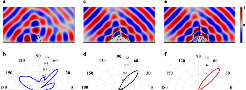
www.nature.com/scientificreports/
Figure 1. A schematic of (a) conventional carpet cloak and (b) NCAC for arbitrary object. The desired non-
closed carpet cloak has an acoustically equal signature with its corresponding conventional one. So, the incident
wave is reflected from the non-closed device as a reflecting plane, without any perturbation.
in airborne acoustics, perforated plastic plates have been applied for 2 D29 and 3 D30 ground plane cloaks and for
underwater acoustics, steal s trips31 and brass p
lates32 have been proposed. In addition, acoustic unidirectional
cloaks were implemented via composites of metals and porous materials for a multi-layered host medium33 and
meta-fluid structured by slab-shape units for air host34.
Although considerable progress has been made in invisibility cloaks, all conventional cloaking devices are
“interior” cloaks and thus prevent the target from interacting with outer world, which is a restriction for the
use of these applicable devices. In order to obviate this drawback, Lai et al.35 presented "external" cloaking and
illusion devices for the EM framework. Because of relevant acoustic demands, not long after the first proposal,
the idea was extended to acoustics by Zhu et al.36. The key enabling feature of designing such external or “non-
closed” invisibility devices is the complementary media concept, which is designed to conceal a predefined
object37–40. However, complementary media based cloaks depend on the shape and material properties of the
hidden object41,42. Therefore, any changes in description of object or any movements disturb the cloaking effect.
Consequently, the dependence of the cloaking device on target and inevitable inhomogeneity of obtained mate-
rials are the remaining challenges that make the implementation of conventional external cloaks practically
nonrealistic.
Differ from conventional design, in this paper; we design non-closed acoustic cloaks (NCACs), in which their
materials are feasibly independent of the target geometry and its constitutive materials. The proposed technique
is based on applying sequential linear transformations to create a non-closed invisible region positioned on a
reflecting plane. Therefore, any standing or moving object in the hidden region will be acoustically invisible
without being blinded. Due to the nature of linear coordinate transformation, the obtained materials of NCAC
are homogeneous which results in easy to fabricate non-closed carpet cloaks. Moreover, the idea of non-closed
devices is further extended to design a free space unidirectional acoustic cloak that can conceal any arbitrary
objects. The full wave numerical simulations using COMSOL finite element solver verify the expected behavior
of NCACs. Finally, to give a more realistic point of view, the required constitutive materials are realized with the
aid of non-resonant acoustic meta-atoms.
Design and theory
Non‑closed carpet cloak. To start with a conception of idea, it is well understood that the conventional
carpet cloak18 has a hidden region underneath a sound hard boundary bump where any arbitrary object located
becomes invisible. The main purpose is to design an acoustic cloak, which, in addition to attempting to avoid
enclosing objects, its constitutive parameters being independent of the material, geometry and position of
objects. Figure 1 illustrates the equivalence between the behavior of the desired non-closed device and its cor-
responding conventional one, where the reflected wave of the whole NCAC and neighbor target is not disturbed.
At the first step, the conventional carpet cloak18 will be proposed. Without loss of generality, the problem
is discussed in 2D framework while
it could be extended to 3D case. As demonstrated
in
Fig. 2a,b, the triangle
BCD in reference space x0 , y0 is mapped to the quadrilateral BCDA in real space x1 , y1 . Therefore, any object
located beneath the BAD sound hard boundary (SHB) bump becomes invisible. At the second step, the existing
SHB in the carpet cloak is physically eliminated by utilizing a linear folded transformation. The resulted folded
medium is a type of complementary media35 and is actually an SHB mimicking structure, without any imposed
sound hard boundary condition. Considering the geometrical symmetry of the scheme, the problem is discussed
only in the left half space of the reference and real spaces and a same method is applied to the right
side. Analyti-
cally, a linear coordinate
transformation that maps KBE region in the reference space x1 , y1 to KBA region
in the real space x2 , y2 folds the ground plane boundary BE to AB and makes an effective SHB on AB , as shown
in Fig. 2c. Hence, the folded medium creates an illusionary SHB bump and regenerates the cloaking effect of the
conventional carpet cloak without making any disturbance in the scattered wave. From now on, for brevity, we
call the domain mimicking the sound hard boundary condition as “spoof sound hard boundary” (SSHB) and
the carpet cloak without physical SHB bump as the carpet cloak with SSHBs.
Scientific Reports | (2021) 11:1845 | https://doi.org/10.1038/s41598-021-81331-3 2
Vol:.(1234567890)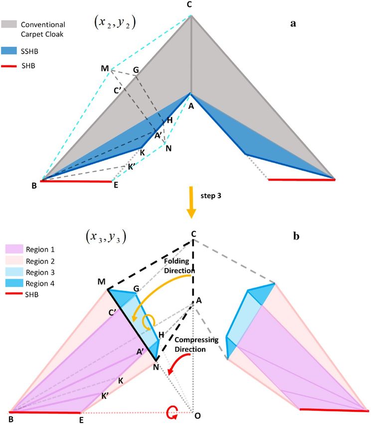
www.nature.com/scientificreports/
Figure 2. Schematic diagram of first and second steps to NCAC design. (a) The reference space. (b)
Conventional carpet cloak’s scheme. (c) The spoof sound hard boundary folds the ∆KBE region in (x1, y1) space
to ∆KBE in (x2,y2) space and makes an illusionary sound hard boundary condition on AB boundary that is
shown by red dashed lines.
In order to verify the effect of carpet cloak with SSHBs, numerical simulations are carried out using the
COMSOL Multiphysics finite element solver. All simulations are performed by adopting the acoustic pressure
field in the frequency of 3.34 kHz, and the host medium is chosen as air with ρ0 = 1 kg/m3 and c0 = 343 m/s
values for mass density and speed of sound, respectively. It is worth to mention that, due to the frequency inde-
pendence of transformation acoustics m ethod1–3, our design strategy is valid for any desired operating frequency
and the chosen frequency, is completely arbitrary. By taking the left side of problem’s geometry as the reference,
at the first and second steps of the design, the acoustic
constitutive materials for conventional
cloaks and the
1.2871 −1.2146 −16.0124 13.0663
SSHB region are ρ cloak = ρ0 , κcloak = 1.9231κ0 and ρ SSHB = ρ0 ,
−1.2146 1.9231 13.0663 −10.7247
κSSHB = −0.0714κ0, where ρ0 and κ0 densities and bulk modulus of the background medium, respectively. The
geometric parameters and derivation of the acoustic properties are detailed in the next section. The performance
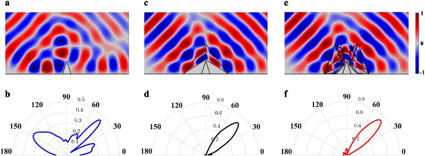
of the carpet cloak with SSHBs comparing with the conventional carpet cloak is demonstrated in Fig. 3a–f. The
near-field and far-field distribution of pressure fields of an object located on the reflecting plane is shown in
Fig. 3a,b, respectively. It is obvious that the presence of object disturbs the reflecting wave. In Fig. 3e,f, the carpet
cloak with SSHBs is used to make the object invisible, whose scattering is closely similar to that of the conven-
tional carpet cloak depicted in Fig. 3c,d. All the aforementioned simulations verify the idea of the illusionary
SHB bump and prove the validity of the carpet cloak with SSHBs.
Finally, we can open a window in the carpet cloak with SSHBs to make its hidden region non-closed. Sub-
sequently, at the third step, the carpet cloak with SSHBs and its surrounding
fluid in the reference space x2 , y2
(Fig. 4a), are compressed to smaller domains in the real space x3 , y3 , as shown in Fig. 4b. For detail, a linear
transformation that maps the OCB region to the OC ′ B, as illustrated by red arrows in Fig. 4b, compresses the
carpet cloak with SSHBs to non-closed regions depicted by region 1. Similarly, the BMC and ENA regions of
the surrounding host fluid are also compressed to BMC ′ and ENA′ domains denoted by region 2 in order to
35,43
satisfy the matching c ondition
. Thereupon, the compressing transformations map NA , AC
and CM bounda-
ries in the reference space x2 , y2 to NA′ , A′ C ′ and C ′ M boundaries in the real space x3 , y3 .
In the coordinate transformation frame, by mapping the carpet cloak with SSHBs to the compressed regions,
the path of the wave and outer boundaries of the structure in the reference space follow the compressing trans-
formation in the real space and are mapped to transformed lines in compressed domains. In order to restore
the path of wave, other folded regions are also utilized. The added domains, which are denoted by regions 3 and
4 shown in Fig. 4b, are a type of complementary media35 that convey the route of wave in the real space to the
compressed space by employing a linear transformation. The linear coordinate mapping folds the black dashed
lines representing the reference space to black solid lines in the real space. The significant result of this mapping
is the invariance of waves’ path from the reference space to the real space (Fig. 4b). Another remarkable implica-
tion of complementary regions is mapping of each outer boundary to itself, which results in satisfaction of the
matching condition35,43. Finally, the incident acoustic fields are conveyed to the compressed domains and track
the compression direction, bypass the cloaked region and are scattered as that in the reference space.
Scientific Reports | (2021) 11:1845 | https://doi.org/10.1038/s41598-021-81331-3 3
Vol.:(0123456789)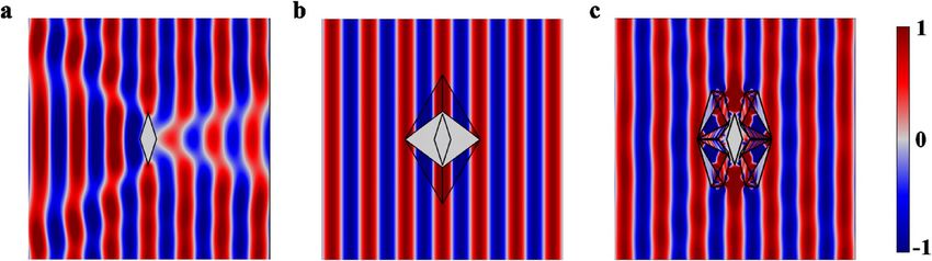
www.nature.com/scientificreports/
Figure 3. Comparison between the field distribution of target, conventional carpet cloak and the carpet cloak
with SSHBs. (a,b) The near field distribution and far field scattering pattern of the object with sound hard
boundaries. (c,d) The near field distribution and far field scattering pattern of conventional carpet cloak. (e,f)
The near field distribution and far field scattering pattern of the carpet cloak with SSHBs. It can be seen that the
results in (c,d) and (e,f) are closely similar to each other.
To mathematically restate the complementary regions, firstly, the complementary medium GHA′ C ′ denoted
by region 3 in Fig. 4b is obtained by mapping OGC in the reference space to OGC ′ in the real space. In fact,
region 3 folds the AC boundary in the reference space to A′ C ′ in the real space and GH boundary to itself, as
illustrated by yellow arrows in Fig. 4b. Similarly, the complementary media of the compressed surrounding
host fluid, denoted by region 4 in Fig. 4b, are achieved by mapping GMC and HNA in the reference space,
respectively to GMC ′ and HNA′ in the real space. The obtained material of GMC ′ region folds MC to MC ′
and MG to itself. In the same manner, the material of HNA′ region folds NA to NA′ and HN to itself. In sum-
mary, the employed linear coordinate transformations to achieve complementary materials drawn by regions
3 and 4 are chosen in a way that MC , NA and AC dashed line boundaries in the reference space, respectively
fold to MC ′ , NA′ and A′ C ′ solid line boundaries in the real space and all outer boundaries of the real space, i.e.
MG , GH and HN are mapped to themselves (Fig. 4b). As a result, the compressed structure in the presence of
complementary materials is matched to the host medium. Therefore, the compounded compressed regions and
complementary materials have an identical scattering effect with the conventional carpet cloak in the reference
space or equally, with a reflecting plane.
By applying the compression and complementing transformations (the steps illustrated in Fig. 4), the neces-
sitating homogeneous constitutive parameters are obtained for each region, which are given in Table 1. More
detailed explanations and derivation of data presented in Table 1, have been proposed in Supplementary Mate-
rial 1.
Recently, the acoustic metamaterial technology has been the subject of numerous r esearches44–48. These studies
show promising results for realization of anisotropic media which are presented in Table 1. The detailed informa-
tion of geometry and constructive materials is also supported in the next section. In order to provide more intui-
tive perception of the designed NCAC, numerical simulations are performed. In Fig. 5, the numerical simulation
results are demonstrated to compare the scattering pattern of the object with and without the non-closed carpet
cloak. Figure 5a,b respectively display the near-field distribution and far-field scattering pattern of an object with
SHB boundaries under the excitation of a Gaussian beam propagating at the angle of π/4 which disturbs the
reflected wave. As demonstrated in Fig. 5e,f, the presence of the designed NCAC adjacent to the object restores
the pressure field distribution and far-field pattern the same as the conventional carpet cloak (shown in Fig. 5c,d).
It is obvious that due to the presence of SSHB, the incident fields do not penetrate the hidden region. Because of
this feature, the target shape and its constitutive materials do not affect the cloaking behavior of the non-closed
structure. Therefore, the significant effect of the device is to hide an arbitrary object without making it blinded.
The simulation results decisively confirm the identical behavior of the designed non-closed carpet cloak with
the original carpet cloak. Using homogeneous materials is another supreme benefit that facilitates realization of
non-closed invisibilities. It is worth mentioning that there is a tradeoff between the extent of the created window
on the cloaking device and difficulty of the realization process. If the cloaking shell is compressed to a highly
smaller region, it looks more fascinating and is really toward fictions; however, complementary materials take
higher values of negative constitutive parameters and implementation of materials will become harder.
Theories and coordinate transformations. In this section, we present mathematical derivation of the
proposed sequential-step coordinate transformations to design of non-closed carpet cloak that is schematically
illustrated in Fig. 4. For convenience, the left side of the structure is considered and all relations can be extended
to the right side. The corresponding transformation equation for the first designing step, which represents the
Scientific Reports | (2021) 11:1845 | https://doi.org/10.1038/s41598-021-81331-3 4
Vol:.(1234567890)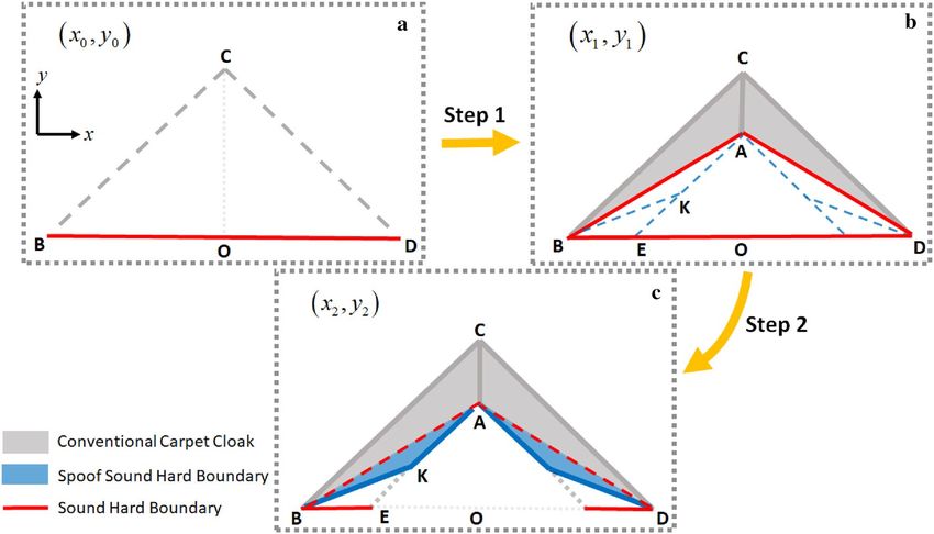
www.nature.com/scientificreports/
Figure 4. Schematic diagram of the proposed object independent non-closed carpet cloak. (a) Carpet cloak
with SSHBs. In order to make a window on this structure, the trapezoidal region AEBC and its surrounding
fluid (dashed light blue lines) in the reference space (x2,y2) are going to be compressed to smaller domains. (b)
Non-closed carpet cloak. The trapezoidal domain AEBC, is compressed to the smaller purple trapezoid denoted
by region 1 in real space (x3,y3) and the surrounding host medium, is also compressed to the melon domains
named region 2. Blue domains show the complementary materials. The black dashed line boundaries represent
the original boundaries before compressing. The incident wave that meeting the dashed lines, is routed to the
solid lines by complementary domains denoted by regions 3 and 4. Significant result of this transformation is
that the signature of the created window on conventional carpet cloak is canceled. Therefore, the whole structure
is matched to host fluid and acts like an illusionary single reflecting plane.
mapping of a reflecting plane in the reference space x0 , y0 to a SHB bump in the real space denoted by x1 , y1
(as depicted in Fig. 2), can be expressed as:
x1 = x0
BOC → BAC :
y1 =
1
x0 + 1 −
YA
y0 + YA (1)
mAB YC
wherein Y A and YC are the ordinates of A and C points in Fig. 2 and mAB is the inverted slope of AB or
(XA − XB ) (YA − YB ). Generally, each point is determined as (Xi , Yi ) where the subscript of i denotes the points’
name. Moreover, the parameter “m” denotes the inverted slope of the line labeled with its index. Due to the
acoustic coordinate transformation t heory3, constitutive
parameters for the resultant conventional cloak are
obtained from the Jacobin matrix J = ∂(x1 , y1 ) ∂(x0 , y0 ) as follows:
� xx xy � � �
ρcloak ρcloak J + m2AB J0−1 −mAB J0−1
ρ cloak = det(J1 )(J1−1 )T ρ0 (J1−1 ) = = ρ0 0
xy yy
ρcloak ρcloak −mAB J0−1 J0−1 (2)
−1 −1
κcloak = κ0 det (J1 ) = κ0 J0
wherein ρ0 and κ0 are the mass density and bulk modulus of the host fluid and J0 = YC (YC − YA ). For the
second step depicted in Fig. 2a,b, the transformation function related with the SSHB region is given by:
Scientific Reports | (2021) 11:1845 | https://doi.org/10.1038/s41598-021-81331-3 5
Vol.:(0123456789)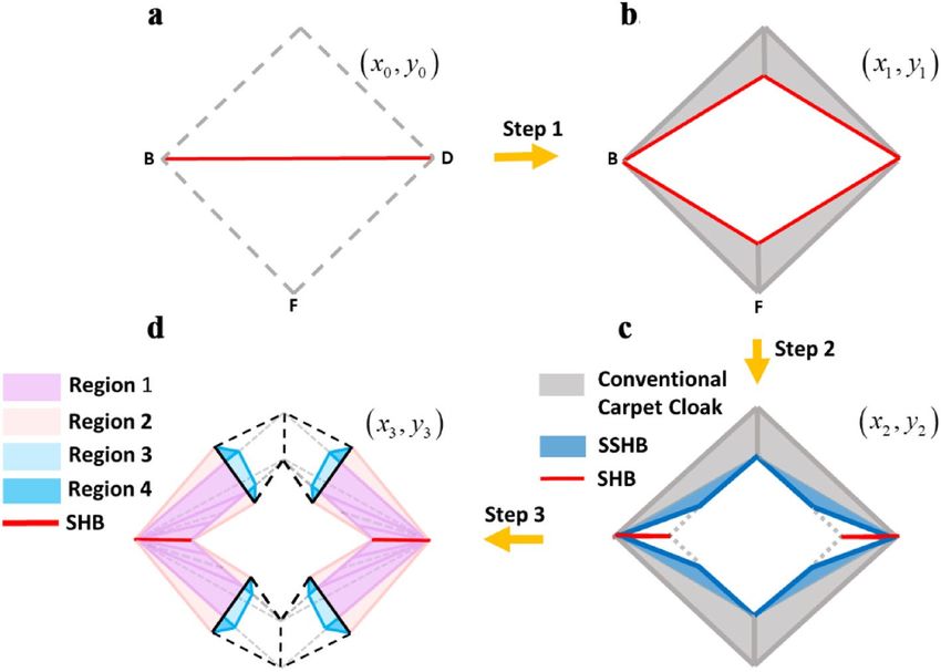
www.nature.com/scientificreports/
0.8703 −0.8978
ρ BA′ C ′ = ρ0 −0.8978 2.0752 , κBA′ C ′ = 2.8441κ0
0.6762 0.2461
Region 1 ρ BK ′ E = ρ0 0.2461 1.5685 , κBK ′ E = 1.4789κ0
−10.8272 9.1255
ρ BA′ K ′ = ρ0 9.1255 −7.7837 , κBA K = −0.1056κ0
′ ′
3.6440 −0.0305
ρ BMC ′ = ρ0 −0.0305 0.2747 , κBMC ′ = 1.4789κ0
Region 2
0.4298 −0.2741
ρ ENA′ = ρ0 −0.2741 2.5015 , κENA′ = 1.4789κ0
−5.3226 0.7788
Region 3 ρ GHC ′ A′ = ρ0 0.7788 −0.3018 , κGHC A = −1.3897κ0
′ ′
−1.2121 −0.3662
ρ MC ′ G = ρ0 −0.3662 −0.9356 , κMC ′ G = −1.3897κ0
Region 4
−7.6589 1.8469
ρ NA′ H = ρ0 1.8469 −0.5759 , κNA′ H = −1.3897κ0
Table 1. The constitutive materials of the NCAC’s regions.
Figure 5. Simulation results of non-closed carpet cloak. (a,b) Near field distributions and far field scattering
pattern of the target with sound hard boundaries that is located on the reflecting plane. The scattered field of
reflecting plane is disturbed in the presence of the target. (c,d) Near field distributions and far field scattering
pattern of the conventional carpet cloak. (e,f) Near field distributions and far field scattering pattern of the target
near the non-closed carpet cloak. The non-closed device restored the scattering pattern of the object as well
as the reflecting plane. It is also similar to field distribution of the conventional structure, which illustrates the
validity of the fenestrated carpet cloak.
x2 = mABm−m AB
x1 + −mAE mKB
m −m y1 + m
−mAB XE
−m
(3)
AE
AB AE AB
AE
KBE → KBA :
1 mAE
−XB
y2 = mAB −m AE
x1 + 1 − m AB −m AE
y1 + m AB −m AE
The above transformation
function folds the KBE region in the reference space x1 , y1 to the KBA region
in the real space x2 , y2 and makes an illusionary SHB on the AB boundary as illustrated in Fig. 2c. By employing
the corresponding Jacobin matrix, the constitutive parameters of the SSHB region are obtained as:
� �
� xx xy � (1+(mBA −mEA −mKB )2 ) mKB XE (mBA −mEA −mKB )+XB
mAB (mBA −mEA −mKB )+mAE mAB − XB (mBA −mEA −mKB )−XE mAB
ρSSHB ρSSHB
ρ = xy yy = ρ
SSHB 0 XB2 +m2KB XE2
ρSSHB ρSSHB − XmBKB(mXBA
E (mBA −mEA −mKB )+XB
−mEA −mKB )−XE mAB − XB (mBA −mEA −mKB )−XE mAB (4)
2
κ (mBA −mEA )
SSHB =κ 0 mAB (mBA −mEA −mKB )+mAE mAB
Then, corresponding to the third step illustrated
in Fig. 4a,b, the transformation equation that maps the carpet
cloak with SSHBs
in the reference space x2 , y2 to non-closed compressed regions denoted by region 1 in the
real space x3 , y3 is expressed as follows:
Scientific Reports | (2021) 11:1845 | https://doi.org/10.1038/s41598-021-81331-3 6
Vol:.(1234567890)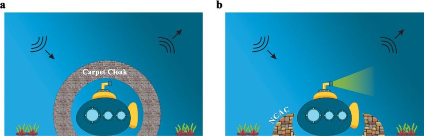
www.nature.com/scientificreports/
x3 = x2 + kmOC ′ y2
OCB → OC ′ B :
y3 = ky2 (5)
Y
where k = YCC′ , represents the compressing ratio. The above transformation function gives the material properties
of each different part of region 1 (Fig. 4b) as:
� xy �
xx
kρcloak xx
ρcloak − kmOC ′ ρcloak 1
ρ ′
BA C ′ = xy xx xx + k−1 ρ yy xy , κBA′ C ′ = κcloak
ρcloak − kmOC ρcloak kmOC ′ ρcloak cloak − 2m OC ′ρ
cloak k
� xy �
xx
kρSSHB xx
ρSSHB − kmOC ′ ρSSHB 1
ρ BK ′ A′ = xy xx xx yy xy , κBK ′ A′ = κSSHB (6)
ρSSHB − kmOC ′ ρSSHB kmOC ′ ρSSHB + k−1 ρSSHB − 2mOC ′ ρSSHB k
� �
k −kmOC ′
, κBEK ′ = k1 κ0
ρ BEK ′ = ρ0
2 −1
−kmOC ′ kmOC ′ + k
Similarly, the compression transformation functions are applied to the surrounding
host fluid in order to
achieve region
2
illustrated in Fig. 4b. The BMC in the reference space x2 , y2 is compressed to BMC ′ in the
real space x3 , y3 with the transformation function:
XB YM − XB YC + XM YC − XC ′ YM XM XC ′ − XB XC ′
x3 = x2 + y2
0 0
a0 0 b
XB XC ′ YM − XB XC YM
+
BMC → BMC ′ : 0
c0
YM YC − YM YC ′ XB YM − XB YC ′ + XM YC ′ XB YM YC ′ − XB YM YC
y3 = x2 + y2 +
0 0 0
d0 e0 f0
(7)
wherein 0 = XB YM − XB YC + XM YC − X C YM . In
a similar manner, △ ENA in the reference space x2 , y2 is
also compressed to △ ENA′ in the real space x3 , y3 by following coordinate transformation:
−XE YA + XN YA − XA′ YN + XE YN XN XA′ − XE XA′ XE XA′ YN
x3 = x2 + y2 +
1 1 1
a 1 b c1
ENA → ENA′ :
YN YA′ − YN YA
XN YA′ − XE YA′ + XE YN
1
XE YA′ YN − XE YA YN
y3 = x2 + y2 +
1 1 1
d1 e1 f1
(8)
that 1 = XN YA − XE YA + XE YN − XN YE . According to Eqs. (7) and (8), the constitutive materials of △ ENA′
and △ BMC ′ that construct region 2 in Fig. 4b are expressed as:
2 2
d0 +e0 a0 d0 −b0 e0
1
ρ BMC ′ = ρ0 a0 e0 −b0 d0 a0ae02−b 0 d0 , κ
2 BMC ′ = a0 e0 −b0 d0 κ0
0 +b0
a0 d0 −b0 e0
a0 e0 −b0 d0 a0 e0 −b0 d0
(9)
d12 +e12 a1 d1 −b1 e1
a1 e1 −b1 d1 a1 e1 −b1 d1 1
ρ ′ = ρ0 , κENA′ =
a1 e1 −b1 d1 κ0
ENA a12 +b12
a1 d1 −b1 e1
a1 e1 −b1 d1 a1 e1 −b1 d1
Subsequently, the complementary medium GHA′ C ′ denoted by region 3 in Fig. 4b is derived by applying the
transformation function:
mOC ′
x3 = 1 − k mOG
x2 + kmOC y2
′
�OGC → �OGC ′ :
1
(10)
y3 = mOG (1 − k) x2 + kmOC ′ y2
which folds the GH boundary to itself and AC to A′ C ′ . Equation (10) gives the material properties of the polygon
region GHC ′ A′ denoted by region 3 in Fig. 4b as follows:
−k2 m2OC ′ m2OG −(k−1)2 k2 m2OC ′ m2OG −(k−1)(mOG −kmOC ′ )
ρ kmOC′ mOG (1−k+kmOC′ −mOG )
GHC ′ A′ = ρ0 k2 m2 ′ m2 −(k−1)(mOG −km ′ )
kmOC ′ mOG (1−k+kmOC ′ −mOG )
−k2 m2OC ′ m2OG −(mOG −kmOC ′ )2
OC OG OC (11)
km OC ′ m OG (1−k+km OC ′ −m OG ) km OC ′ mOG (1−k+kmOC ′ −mOG )
−κ0 mOG
κGHC ′ A′ = kmOC′ mOG (1−k+kmOC′ −mOG )
Finally, transformation
equations are applied to the specify region 4 in Fig. 4b. The GMC domain of region
′
4 in the real space x3 , y3 is determined by the transformation function:
Scientific Reports | (2021) 11:1845 | https://doi.org/10.1038/s41598-021-81331-3 7
Vol.:(0123456789)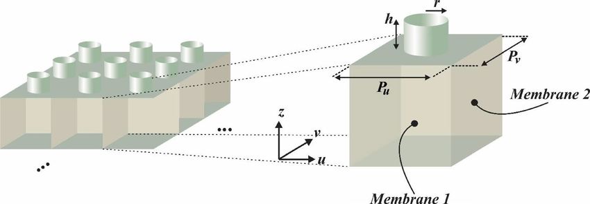
www.nature.com/scientificreports/
XM YC − XC ′ YM − XM YG + XG YM − XG YC + XC ′ YG XM XC ′ − XC ′ XG
x3 = x2 + y2
2 2
a2 b2
XC ′ XG YM − XM XC ′ YG
+
2
c2
GMC → GMC ′ :
YM YC − YM YC ′ − YC YG − YC ′ YG XM YC ′ − XM YG + XG YM − XG YC ′
y3 = x2 + y2
2 2
2 d e2
XM YC YG − XG YM YC − XM YC ′ YG + XG YM YC ′
+
2
f2
(12)
wherein 3 = XH YA − XN YA + XN Y H − X Y
H N . The coordinate transformation
described in Eq. (12) folds the
MC boundary in the reference space x2 , y2 to MC ′ in the real space x3 , y3 and
also folds the outer boundary
MG to itself. Moreover, the HNA′ domain of region 4 in the real space x3 , y3 is determined by the transfor-
mation equation:
−XN YA + XA′ YN + XH YA − XA′ YH + XN YH − XH YN XH XA′ − XA′ XN
x3 = x2 + y2
3 3
a3 b3
XA′ XN YA − XA′ XH YN
+
3
c3
HNA → HNA′ :
−YA YN + YA′ YN + YA YH − YA′ YH −XN YA′ + XH YA′ + XH YN − XH YN
y3 = x2 + y2
3 3
3 d e3
XH YA YN − XN YA YH + XN YA′ YA − XH YN YA′
+
3
f3
(13)
with the assumption of 2 = XM YC − XM YG + XG YM −
XG YC . The coordinate transformation
presented in
Eq. (13) folds the NA boundary in reference space x2 , y2 to NA′ in the real space x3 , y3 and folds the outer
boundary HN to itself. Equations (12) and (13), respectively give the material properties of △ GMC ′ and △ HNA′
domains of region 4 as follows:
2 2
d2 +e2 a2 d2 −b2 e2
1
ρ GMC ′ = ρ0 a2 e2 −b2 d2 a2ae22−b 2 d2 , κ
2 GMC ′ = a2 e2 −b2 d2 κ0
a2 d2 −b2 e2 2 +b2
a2 e2 −b2 d2 a2 e2 −b2 d2
2 2 (14)
d3 +e3 a3 d3 −b3 e3
a e −b d a e −b d 1
, κHNA′ =
ρ HNA′ = ρ0 a3 d3 −b3 e3 a32 +b32 a3 e3 −b3 d3 κ0
3 3 3 3 3 3 3 3
a3 e3 −b3 d3 a3 e3 −b3 d3
The presented three design steps illustrated in Figs. 2 and 4 to achieve a non-closed carpet cloak are dem-
onstrated by mathematical terminology (Eqs. 1–14). As illustrated in the next section, all discussions can be
repeated to designing the non-closed unidirectional cloak because of its similar design steps with the carpet
cloak. The design method also can be extended to achieve a larger number of windows in the structure and it
could also be applied to other acoustic devices to make them fenestrated. The method could also be generalized
to illusion devices by changing the first reference space in the step 1 (Fig. 2).
Non‑closed unidirectional cloak. It is well understood that carpet cloaks only work in the presence of a
reflecting plane. In order to make it possible to hide an arbitrary object in the free space, the proposed method
is further extended to design a non-closed unidirectional cloak. Analogous to the EM scenario21, designing
acoustic unidirectional cloaks is based on the fact that there is no scattered field when the propagation of acous-
tic wave is parallel to an infinitely thin SHB surface. Figure 6a,b illustrate the idea of unidirectional cloak. As
illustrated, to design such a unidirectional cloak, an SHB diamond hole is made in BCDF domain. For detail, the
reference space is compressed into the real space by mapping an SHB line segment to an SHB diamond in the
interior boundary, while the exterior space is unchanged. Any object located inside the resultant diamond shape
SHB region becomes invisible. Unidirectional free space cloaks as a practical and easy to fabricate alternative
device for ideal free space cloaks have numerous particular applications such as hiding submarines from sonar,
airborne sound cloaking, etc.
In order to make the conventional unidirectional cloak non-closed to outer world, the aforementioned three
design steps, i.e. transforming the structure to the device with SSHBs, compressing and complementing, should
Scientific Reports | (2021) 11:1845 | https://doi.org/10.1038/s41598-021-81331-3 8
Vol:.(1234567890)www.nature.com/scientificreports/
Figure 6. Scheme illustration of the free space fenestrated cloak (a–d) The three design steps. The
unidirectional cloak is achieved by transforming the diamond space specified by grey dashed line to the space
with the diamond shape inner sound hard boundaries. Analogous to the non-closed carpet cloak scenario, firstly
one should use SSHB material for the unidirectional cloak rather than sound hard boundary condition. (d)
Geometry of resulting device. The proposed structure can hide objects located in the host fluid without making
them blinded and the drawn windows of structure, allow transforming of matter and information.
Figure 7. The simulation results of non-closed free space cloak. The near field of (a) object with sound hard
boundaries, (b) the conventional unidirectional cloak, and (c) the target in the presence of non-closed free space
cloak, which is recovered as well as the conventional free space cloaks pattern in (b).
be employed to make windows on the body of it. Due to the structural symmetry of the unidirectional cloak and
similar materials with the carpet cloak, the reference space can be considered as two mirror conventional carpet
cloaks, as illustrated in Fig. 6b. Hence, by passing the same three design steps, the resultant transformation media
will have the similar constitutive materials with the non-closed carpet cloak. In Fig. 6, second and third design
steps are applied to achieve a non-closed unidirectional cloak.
By performing numerical simulations, the directional perfect cloaking effect of the resultant non-closed free
space cloak is verified. Figure 7a–c demonstrate the near field distribution of three cases: an arbitrary object in
free space, conventional and non-closed unidirectional cloaks. The incident plane wave is excited parallel to the
virtual SHB surface. Comparing the results of Fig. 7b,c underlines the closely equivalent signature of the non-
closed cloak and original one.
Consequently, the performance of free space cloak with the advantage of the non-closed structure is veri-
fied. The important prudence is to note that the non-closed free space cloak is prescribed for a specific direc-
tional propagation similar to the conventional one. The proposed non-closed unidirectional cloak possesses
all excellences of the conventional unidirectional cloak, including the object independent performance and
Scientific Reports | (2021) 11:1845 | https://doi.org/10.1038/s41598-021-81331-3 9
Vol.:(0123456789)www.nature.com/scientificreports/
0.3916 0
θ rot = −28.06◦ , ρ BA′ C ′ = ρ0 0 2.5539 , κBA C = 2.8441κ0
′ ′
0.6128 0
Region 1 θ rot = 14.44◦ , ρ BK ′ E = ρ0 0 1.6319 , κBK E = 1.4789κ0
′
−18.557 0
θ rot = 40.26◦ , ρ BA′ K ′ = ρ0 0 −0.0539 , κBA K = −0.1056κ0
′ ′
3.6443 0
θ rot = 0.51◦ , ρ BMC ′ = ρ0 0 0.2744 , κBMC = 1.4789κ0
′
Region 2
0.3941 0
θ rot = −7.41◦ , ρ ENA′ = ρ0 0 2.5372 , κENA = 1.4789κ0
′
−5.4 0
Region 3 θ rot = 8.5◦ , ρ GHC ′ A′ = ρ0 0 −0.18 , κGHC A = −1.3897κ0
′ ′
−1.46 0
θ rot = −34.65◦ , ρ MC ′ G = ρ0 0 −0.68 , κMC G = −1.3897κ0
′
Region 4
−8.11 0
θ rot = 13.77◦ , ρ NA′ H = ρ0 0 −0.12 , κNA H = −1.3897κ0
′
Table 2. The constitutive materials of the NCAC’s regions after diagonalization.
homogeneous-material structure, together with the non-blinded architecture. All these interesting benefits make
the device applicable in free space cloaking practical demands.
Meta‑atom realization
In this section, we propose a possible acoustic metamaterial structure that could be utilized to mimic the consti-
tutive parameters of the NCAC structure. To this end, considering the effective medium t heory44–48, we design
meta-atoms whose effective properties are matched with the required data presented in Table 1. At the first,
the off-diagonal components of the mass density tensor should be eliminated. It is worth mention that any off-
diagonal symmetric tensor can be transformed to a diagonal one with a proper rotation around its principal a xis49.
To this aim, the obtained tensors presented in Table. 1 will be multiplied by the rotation matrix (θ is unknown
and must be calculated).
ρu 0 cos θ − sin θ ρ ρ cos θ sin θ t t
= × xx xy × = 11 12 (15)
0 ρv sin θ cos θ ρxy ρyy − sin θ cos θ t21 t22
where
ρxx − ρyy
t12 = t21 = sin 2θ + ρxy cos 2θ (16)
2
In Eq. (15) v and u denote the axes of the rotated coordinate. In order to find the rotation angle which will
cause the tensor
of Eq.
(15) to be diagonal, we should solve t12 = t21 = 0 which consequently results in
−2ρ
θ = 12 arctan ρxx −ρxyyy and the components of anisotropic mass density in new coordinate, can be calculated as
ρu = cos2 θρxx + sin2 θρyy + 2 sin θ cos θρxy
ρv = sin2 θρxx + cos2 θρyy − 2 sin θ cos θρxy (17)
By applying aforementioned coordinate rotation, the diagonalized constitutive parameters are presented in
Table 2.
As can be seen in Table 2, the required parameters for regions 3 and 4 and △ BA′ K ′ region, are double negative
value for mass density tensor and also have negative bulk modulus. A prevalent way to implement homogene-
ous double-negative acoustic media is to use resonant membrane type meta-atoms. However, the inevitable loss
and dispersion of the resonant structures, extremely limits the efficiency and operating frequency band of the
homogenized medium and exacerbates the unwanted couplings. To go beyond these restrictions, we utilize the
quasi two-dimensional non-resonant meta-atom proposed in48. As shown in Fig. 8a, the meta-atom consists of
an elastic membrane and a side branch with open end. By assigning different thicknesses to membranes’ faces
in u and v directions (thu and thv , respectively), anisotropic and negative density can be achieved simultane-
ously. In addition, the bulk modulus is tuned by the geometry of the side branch. The wide bandwidth of this
meta-atom is resulted from its large resonance damping. The membrane material is assumed to be aluminum
with Young modulus of 70 GPa, the Poisson ratio of 0.33 and the mass density of 2700 kg/m3 and the tension on
the membrane is assumed to be zero. The dimensions and geometrical features of the meta-atom are described
in the Figure caption and the retrieved parameters for all regions are shown in Fig. 8b–i. It can be seen that the
retrieved results match well with the required parameters at the frequency of 3.34 kHz . Due to the non-resonant
properties of the meta-atom, the imaginary parts of the retrieved parameters are negligible. It is obvious that the
meta-atom exhibits negative mass density and bulk modulus in a broadband frequency range without relying on
Scientific Reports | (2021) 11:1845 | https://doi.org/10.1038/s41598-021-81331-3 10
Vol:.(1234567890)www.nature.com/scientificreports/
a
b c
d e
Figure 8. (a) Scheme illustration of the utilized non-resonant meta-atom. The membrane in repeated along
u and v directions with periodicity pu = pv = 4 mm. The retrieved parameters for all regions are shown in
(b–i). (b–d) Real parts of retrieved parameters of region 1. For BA′ C ′, the thickness of membranes’ faces
are thu = 6.368 µm and thv = 5.387 µm. The radius and height of the side branch are r = 0.4 mm and
h = 2.958 mm, respectively. For BK ′ E : thu = 5.859 µm, thv = 6 µm, r = 0.4 mm and h = 6.11 mm. For
BA′ K ′, thu = 10.5 µm, thv = 6.53 µm, r = 1.2 mm and h = 1 mm. (e,f) Real parts of retrieved parameters
of region 2. For BMC ′: thu = 4.603 µm, thv = 6.41 µm, r = 0.4 mm and h = 6.11 mm and for ENA′,
thu = 6.36 µm, thv = 5.4 µm, r = 0.4 mm and h = 6.11 mm. (g) Real parts of retrieved parameters of region
3. For GHC ′ A′ region, thu = 8.02 µm, thv = 6.57 µm, r = 0.4 mm and h = 0.94 mm. (h,i) Real parts of
retrieved parameters of region 4. For MC ′ G: thu = 6.986 µm, thv = 6.471 µm, r = 0.4 mm and h = 0.94 mm
and for NA′ H , thu = 8.611 µm, thv = 6.553 µm, r = 0.4 mm and h = 0.94 mm.
Scientific Reports | (2021) 11:1845 | https://doi.org/10.1038/s41598-021-81331-3 11
Vol.:(0123456789)www.nature.com/scientificreports/
f g
h i
Figure 8. (continued)
the resonance and the retrieved parameters, change smoothly with respect to the frequency which minimizes the
coupling effects. These results, therefore demonstrate the possibility of realization of the designed non-closed
acoustic cloaking devices. The finite element analysis software COMSOL is used for the parameter retrieval
simulations.
Discussion and conclusion
To summarize, we design and numerically demonstrate a new strategy to achieve acoustic external cloaking
without full enclosure by applying sequential-step linear coordinate transformations. The cloaking effect of the
proposed non-closed devices is independent of the shape and constitutive material of the target. Therefore, the
target can alter shape or move in the hidden region and transform information with outer world without being
blinded. There is a tradeoff when the window(s) created on the structure are extended, which leads to increasing
the value of negative constitutive parameters. The presented approach surmounts resorting to spatially-varying
constitutive parameters and object-dependent performance of the cloaking devices. The homogeneous material
parameters of the proposed devices significantly facilitate the realization of acoustic external cloaking devices.
To give a more realistic point of view, the required materials for cloaking devices are realized with the aid of
non-resonant acoustic meta-atoms. Due to these benefits, the proposed structures could find applications in
varied scenarios such as making submarines invisible from sonar with non-blinded or fenestrate structures. As
a proof-of-concept demonstration, the proposed NCAC design is carried out at a selected frequency. It should
be noted that the strategy itself is not dependent on the choice of the frequency and the design can be updated
for any desired operating frequency. The impact of loss is minimized due to the non-resonance meta-atom. As
the meta-atoms are dispersive, the bandwidth of the device can be limited for a practical design. To increase the
bandwidth, achromatic metamaterials with inverse design techniques may be used to decrease the frequency
dependence of the effective properties. In addition, based on the effective medium theory, the dimension of
meta-atom must be much smaller than the operating wavelength. To apply the concept to higher frequencies,
the size of meta-atoms should be decreased which is feasible due to the advanced technology of fabrication. The
Scientific Reports | (2021) 11:1845 | https://doi.org/10.1038/s41598-021-81331-3 12
Vol:.(1234567890)www.nature.com/scientificreports/
presented method can also be applied to other acoustic devices, such as acoustic cavities, waveguides, illusion
devices, etc., to make them non-closed to outer world that could be useful in future acoustic demands.
Received: 20 April 2020; Accepted: 5 January 2021
References
1. Pendry, J. Controlling electromagnetic fields. Science 312, 1780–1782 (2006).
2. Cummer, S. & Schurig, D. One path to acoustic cloaking. New J. Phys. 9, 45–45 (2007).
3. Chen, H. & Chan, C. Acoustic cloaking in three dimensions using acoustic metamaterials. Appl. Phys. Lett. 91, 183518 (2007).
4. Cummer, S. et al. Scattering theory derivation of a 3D acoustic cloaking shell. Phys. Rev. Lett. 100, 20 (2008).
5. Chen, Y. et al. Broadband solid cloak for underwater acoustics. Phys. Rev. B 95, 20 (2017).
6. Pendry, J. & Li, J. An acoustic metafluid: Realizing a broadband acoustic cloak. New J. Phys. 10, 115032 (2008).
7. Sanchis, L. et al. Three-dimensional axisymmetric cloak based on the cancellation of acoustic scattering from a sphere. Phys. Rev.
Lett. 110, 20 (2013).
8. García-Chocano, V. et al. Acoustic cloak for airborne sound by inverse design. Appl. Phys. Lett. 99, 074102 (2011).
9. Wong, Z. et al. Optical and acoustic metamaterials: Superlens, negative refractive index and invisibility cloak. J. Opt. 19, 084007
(2017).
10. Zhang, S., Xia, C. & Fang, N. Broadband acoustic cloak for ultrasound waves. Phys. Rev. Lett. 106, 20 (2011).
11. Li, J. & Pendry, J. Hiding under the carpet: A new strategy for cloaking. Phys. Rev. Lett. 101, 20 (2008).
12. Ma, H., Jiang, W., Yang, X., Zhou, X. & Cui, T. Compact-sized and broadband carpet cloak and free-space cloak. Opt. Express 17,
19947 (2009).
13. Kallos, E., Argyropoulos, C. & Hao, Y. Ground-plane quasicloaking for free space. Phys. Rev. A 79, 20 (2009).
14. Ma, H. & Cui, T. Three-dimensional broadband ground-plane cloak made of metamaterials. Nat. Commun. 1, 20 (2010).
15. Keivaan, A., Fakheri, M., Abdolali, A. & Oraizi, H. Design of coating materials for cloaking and directivity enhancement of cylin-
drical antennas using transformation optics. IEEE Antennas Wirel. Propag. Lett. 16, 3122–3125 (2017).
16. Zhang, B., Chan, T. & Wu, B. Lateral shift makes a ground-plane cloak detectable. Phys. Rev. Lett. 104, 20 (2010).
17. Luo, Yu. et al. A rigorous analysis of plane-transformed invisibility cloaks. IEEE Trans. Antennas Propag. 57, 3926–3933 (2009).
18. Zhu, W., Ding, C. & Zhao, X. A numerical method for designing acoustic cloak with homogeneous metamaterials. Appl. Phys. Lett.
97, 131902 (2010).
19. Fakheri, M., Abdolali, A., Hashemi, S. & Noorbakhsh, B. Three-dimensional ultra-wideband carpet cloak using multi-layer dielec-
trics. Microw. Opt. Technol. Lett. 59, 1284–1288 (2017).
20. Popa, B. & Cummer, S. Homogeneous and compact acoustic ground cloaks. Phys. Rev. B 83, 20 (2011).
21. Xi, S., Chen, H., Wu, B. & Kong, J. One-directional perfect cloak created with homogeneous material. IEEE Microw. Wirel. Compon.
Lett. 19, 131–133 (2009).
22. Landy, N. & Smith, D. A full-parameter unidirectional metamaterial cloak for microwaves. Nat. Mater. 12, 25–28 (2012).
23. Hu, W., Fan, Y., Ji, P. & Yang, J. An experimental acoustic cloak for generating virtual images. J. Appl. Phys. 113, 024911 (2013).
24. Zhu, R. et al. A broadband polygonal cloak for acoustic wave designed with linear coordinate transformation. J. Acoust. Soc. Am.
140, 95–101 (2016).
25. Zhu, J. et al. Design and analysis of the trapeziform and flat acoustic cloaks with controllable invisibility performance in a quasi-
space. AIP Adv. 5, 077192 (2015).
26. Li, Q. & Vipperman, J. Non-singular three-dimensional arbitrarily shaped acoustic cloaks composed of homogeneous parts. J.
Appl. Phys. 124, 035103 (2018).
27. Chen, J., Liu, J. & Liu, X. Broadband underwater acoustic carpet cloak based on pentamode materials under normal incidence.
AIP Adv. 8, 085024 (2018).
28. Yang, Y., Wang, H., Yu, F., Xu, Z. & Chen, H. A metasurface carpet cloak for electromagnetic, acoustic and water waves. Sci. Rep.
6, 20 (2016).
29. Popa, B., Zigoneanu, L. & Cummer, S. Experimental acoustic ground cloak in air. Phys. Rev. Lett. 106, 20 (2011).
30. Zigoneanu, L., Popa, B. & Cummer, S. Three-dimensional broadband omnidirectional acoustic ground cloak. Nat. Mater. 13,
352–355 (2014).
31. Bi, Y. et al. Experimental demonstration of three-dimensional broadband underwater acoustic carpet cloak. Appl. Phys. Lett. 112,
223502 (2018).
32. Bi, Y., Jia, H., Lu, W., Ji, P. & Yang, J. Design and demonstration of an underwater acoustic carpet cloak. Sci. Rep. 7, 20 (2017).
33. Zhu, J. et al. A unidirectional acoustic cloak for multilayered background media with homogeneous metamaterials. J. Phys. D Appl.
Phys. 48, 305502 (2015).
34. Kan, W., Guo, M. & Shen, Z. Broadband unidirectional invisibility for airborne sound. Appl. Phys. Lett. 112, 203502 (2018).
35. Lai, Y., Chen, H., Zhang, Z. & Chan, C. Complementary media invisibility cloak that cloaks objects at a distance outside the cloak-
ing shell. Phys. Rev. Lett. 102, 20 (2009).
36. Zhu, X., Liang, B., Kan, W., Zou, X. & Cheng, J. Acoustic cloaking by a superlens with single-negative materials. Phys. Rev. Lett.
106, 20 (2011).
37. Liu, B. & Huang, J. Acoustically conceal an object with hearing. Eur. Phys. J. Appl. Phys. 48, 20501 (2009).
38. Yang, J., Huang, M., Yang, C., Peng, J. & Chang, J. An external acoustic cloak with N-sided regular polygonal cross section based
on complementary medium. Comput. Mater. Sci. 49, 9–14 (2010).
39. Li, B. et al. An arbitrary-shaped acoustic cloak with merits beyond the internal and external cloaks. Acoust. Phys. 63, 45–53 (2017).
40. Li, T., Huang, M., Yang, J., Wang, M. & Yu, J. Acoustic external cloak with only spatially varying bulk modulus. Eur. Phys. J. Appl.
Phys. 57, 20501 (2011).
41. Zheng, B. et al. Concealing arbitrary objects remotely with multi-folded transformation optics. Light Sci. Appl. 5, e16177–e16177
(2016).
42. Madni, H., Aslam, N., Iqbal, S., Liu, S. & Jiang, W. Design of a homogeneous-material cloak and illusion devices for active and
passive scatterers with multi-folded transformation optics. J. Opt. Soc. Am. B 35, 2399 (2018).
43. Kildishev, A. & Narimanov, E. Impedance-matched hyperlens. Opt. Lett. 32, 3432 (2007).
44. Fokin, V., Ambati, M., Sun, C. & Zhang, X. Method for retrieving effective properties of locally resonant acoustic metamaterials.
Phys. Rev. B 76, 20 (2007).
45. Popa, B. & Cummer, S. Design and characterization of broadband acoustic composite metamaterials. Phys. Rev. B 80, 20 (2009).
46. Zigoneanu, L., Popa, B., Starr, A. & Cummer, S. Design and measurements of a broadband two-dimensional acoustic metamaterial
with anisotropic effective mass density. J. Appl. Phys. 109, 054906 (2011).
47. Shen, C. et al. Broadband acoustic hyperbolic metamaterial. Phys. Rev. Lett. 115, 20 (2015).
Scientific Reports | (2021) 11:1845 | https://doi.org/10.1038/s41598-021-81331-3 13
Vol.:(0123456789)www.nature.com/scientificreports/
48. Shen, C., Xu, J., Fang, N. & Jing, Y. Anisotropic complementary acoustic metamaterial for canceling out aberrating layers. Phys.
Rev. X 4, 20 (2014).
49. Barati, H., Fakheri, M. & Abdolali, A. Experimental demonstration of metamaterial-assisted antenna beam deflection through
folded transformation optics. J. Opt. 20, 085101 (2018).
Author contributions
Z.B. and M.H.F. conceived the idea and conducted the simulations. M.H.F. and C.S. designed the non-resonant
acoustic meta-atoms. Z.B., M.H.F. and C.S. participated in the analyzing of the results and their corresponding
discussions. Finally, Z.B. wrote the manuscript based on the input from all authors. A.A. concurrently supervised
the project and reviewed each of the early versions of the manuscript.
Competing interests
The authors declare no competing interests.
Additional information
Supplementary Information The online version contains supplementary material available at https://doi.
org/10.1038/s41598-021-81331-3.
Correspondence and requests for materials should be addressed to A.A.
Reprints and permissions information is available at www.nature.com/reprints.
Publisher’s note Springer Nature remains neutral with regard to jurisdictional claims in published maps and
institutional affiliations.
Open Access This article is licensed under a Creative Commons Attribution 4.0 International
License, which permits use, sharing, adaptation, distribution and reproduction in any medium or
format, as long as you give appropriate credit to the original author(s) and the source, provide a link to the
Creative Commons licence, and indicate if changes were made. The images or other third party material in this
article are included in the article’s Creative Commons licence, unless indicated otherwise in a credit line to the
material. If material is not included in the article’s Creative Commons licence and your intended use is not
permitted by statutory regulation or exceeds the permitted use, you will need to obtain permission directly from
the copyright holder. To view a copy of this licence, visit http://creativecommons.org/licenses/by/4.0/.
© The Author(s) 2021
Scientific Reports | (2021) 11:1845 | https://doi.org/10.1038/s41598-021-81331-3 14
Vol:.(1234567890)You can also read