State Acquisition in Computer Networks
←
→
Page content transcription
If your browser does not render page correctly, please read the page content below
State Acquisition in Computer Networks
                                                         Ruairí de Fréin
                                         School of Electrical and Electronic Engineering
                                             Dublin Institute of Technology, Ireland

   Abstract—We establish that State Acquisition should be per-      state into a numeric value; its role is different to monitoring,
formed in networks at a rate which is consistent with the           which is a means for making the acquired state available to the
rate-of-change of the element or service being observed. We         network manager. Fig. 1 demonstrates a generic acquisition-
demonstrate that many existing monitoring and service-level
prediction tools do not acquire network state in an appropriate     monitoring set-up, which is representative of many scenarios.
manner. To address this challenge: (1) we define the rate-of-       An acquisition function observes an element’s state every
change of different applications; (2) we use methods for analysis   Ta seconds; a monitoring agent submits a report to the
of unevenly spaced time series, specifically, time series arising   network manager every Tm seconds based on the acquisition
from video and voice applications, to estimate the rate-of-change   agent’s observations. In many applications, the acquisition and
of these services; and finally, (3) we demonstrate how to acquire
network state accurately for a number of real-world traces          monitoring functions use the same time-step, Ta = Tm ; the
using Greedy Acquisition. The accuracy of State Acquisition is      acquisition agent and monitoring agent are one and the same.
improved when it is performed at a rate which is consistent with       The design of network monitoring algorithms (such as [1])
its rate-of-change. An improvement in representation accuracy of    does not focus on the role of metric acquisition. Linux comes
one order of magnitude is achieved for voice and video streaming    with widely used metric acquisition routines. The assumption
applications; this improvement does not incur any additional
bandwidth or storage cost.                                          is that existing tools can be relied upon to acquire metrics;
   Index Terms—State Acquisition; Network monitoring; Spectral      the role of the monitoring protocol is to determine when
analysis; Period detection.                                         to aggregate the metrics and to deliver them to the network
                                                                    manager. The confidence the monitoring and learning commu-
                      I. I NTRODUCTION                              nities have in these acquisition routines is unwarranted – these
        ANY network management tools use Linux tools for            routines may not be sufficiently accurate for modern network
M       State Acquisition to acquire inputs for higher-level
functions such as network monitoring algorithms [1], service
                                                                    monitoring and learning protocols [11]. The performance of
                                                                    a monitoring function depends on the quality of the data that
level prediction algorithms [2], [3] and resource allocation        it consumes. The increase in dynamicity and heterogeneity
routines [4]. Some examples of these acquisition tools include      of modern networks [12], which makes networks harder to
the System Activity Report (SAR) [5], Nagios [6] and top            manage, exacerbates this problem.
[7] (in association with tools such as netstat and dropwatch).         The problem with off-the-shelf metric acquisition routines
Monitoring tools that use these acquisition methods promise         is that many of them are periodic with a default resolution of
to deliver notifications to the user if the aggregate of some       1 second, for example SAR [5]. Consequently, many network
metric is above a threshold across an entire infrastructure         monitoring routines monitor the network with this temporal
or on a per machine basis [6]. With respect to a cluster            precision limitation [13]. This was one of the reasons (scalabil-
of machines, aggregates in terms of the average, maximum,           ity issues contributed also) why SoundCloud developers devel-
minimum or sum are computed [1] as a function of time               oped their own monitoring solution, Prometheus [8]. Similar
and/or across machines or instances [8]. These types of             in spirit to our approach, Prometheus stores all data that is pe-
notifications are given for a number of different metrics, for      riodically pulled from SoundCloud’s [14] instrumented micro-
example, revenue or data center temperature. Statistics are         services architecture as time series, where time-stamps have
then absorbed by tools such as StatsD [9] and representative        a millisecond resolution and values are 64-bit floats. In order
charts are generated every 10s for example (using tools such        to save disk space, Nagios XI stores performance data in a
as Graphite). This paper considers the validity of current State    Round Robin Database, which consists of performance metrics
Acquisition approaches, which acquire the data for higher-          periodically averaged over 1, 5, 30 and 360 minute time-steps.
level functions such as monitoring, learning, graphing and          We examine if these periodic acquisition approaches yield
problem diagnosis. In particular, we examine methods for            sufficient accuracy.
acquiring and aggregating network metrics in voice and video           In the case of event-based monitoring and learning routines
applications [10].                                                  using SAR [5], there may be a lag of up to 1 second between
   To fix ideas, State Acquisition is defined as a function that    the occurrence of an event and the time a monitoring report
measures the state of a network or service and converts this        is sent in response to it [3]. The descriptor, “event-based”, is
                                                                    inappropriate. The authors of [2] and [3] use SAR to acquire
                                                                    kernel metrics from a video server once per second in order
ISBN 978-3-903176-08-9 c 2018 IFIP                                  to perform client service level prediction, dealing with load-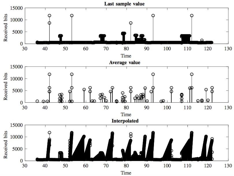
or video frames (that are streamed from a SoundCloud or
Youtube server) are observed at a client machine, the time-
stamps of frame arrivals and the frame-sizes, (t n, x n ), can
be useful for service outage detection. Fig. 2 illustrates a
frame-arrival time-series at a client machine when a podcast is
streamed. When the network is sufficiently well provisioned,
Fig. 1. The role of state acquisition in the monitoring ecosystem: metrics this process has a periodic component. The server periodically
are pushed every Ta seconds to a periodic monitoring gateway, with period sends the client a segment of data, which the client then plays-
Tm , from instrumented systems delivering either long or short lived jobs. out to the user at the sampling rate of the original recording
Periodically acquired observations are stored locally, rules are applied to
them to generate new time series; alerts are triggered; they contribute to [19]. Important statistics such as jitter and packet loss rates
monitoring or querying dashboards; or they are supplied to learning APIs. may be computed from this time-series [18]; however, net-
The performance of these higher-order functions depends on quality of the work anomaly diagnosis may be performed, or service-level
acquired data.
prediction [3], if these time-series are gathered from multiple
network elements at one monitoring/learning gateway [10].
effects in particular in [15]. For a video and voice resource al- This motivates the question: do the acquisition methods that
location application the authors of [4] acquired measurements currently operate at clients allow us to determine (1) the rate
of resource parameters (CPU, RAM, latency and call drops) of change of the observed process and (2) the period of this
every 15s from a Clearwater cloud ISM test-bed, using SNMP process illustrated in Fig. 2? Knowledge of these parameters is
and Cacti [16] to determine how physical resources could be crucial for building a learning function that can predict future
dynamically allocated to virtualized network functions. More network behaviour (cf. [3]).
generally, RTCP [17] is commonly used to provide out-of-band We define a framework for analyzing unevenly spaced time
statistics for RTP sessions by periodically reporting on packet series to answer this question. For N ≥ 1, the space of strictly
counts, packet loss, packet delay variation, and round-trip de- increasing time sequences of length N is denoted: T N = {(t 1 <
lay time to participants in a streaming multimedia session [18]. t 2 < . . . < t N ) : t n ∈ R, 1 ≤ n ≤ N }. More generally, the
The recommended minimum RTCP report interval per station space of strictly increasing time sequences is denoted, T =
is 5 seconds. Nagios’ Remote Plugin Executor periodically ∪∞ N =1 T N . The observation values, x, in computer networks
polls the agent on the remote system for disk usage and are real-valued, R N . Bringing these ideas together, the space
system-load statistics. Now that we have established the central of real-valued, unevenly spaced time series of length N, is
role periodic acquisition and monitoring plays in networks, we TN = T N × R N . Finally, the space of real-valued unevenly
examine the efficacy of periodic State Acquisition. spaced time series is T = ∪∞ N =1 TN . We often need to quantify
We query the acquisition resolution required to monitor the the number of observations in some sequence x, e.g. N =
quality of service received by the client in a video and in a |x|. The sequence of observation times is denoted, T (x) =
voice session. Minimizing network bandwidth usage plays a (t 1, . . . , t N ), and the sequence of observation values of x is
role in determining the acquisition periods of Ta = 1, 5 and 15 V (x) = (x 1, . . . , x N ).
seconds used in the approaches above. Consuming bandwidth
Time series acquisition methods (used by [5],[6] and [7])
with monitoring reports is undesirable; however, reporting the
are used to summarize the performance of network entities,
system state inaccurately is perhaps even more undesirable
so that at times t = nTa , performance can be quantified. Here
than not reporting at all. We examine this trade-off between
n is an integer that denotes the acquisition time index. There
accuracy and bandwidth usage, but also consider whether
are a number of different acquisition methods. The extracted
crucial characteristics of each trace have been preserved by
metrics are passed to a monitoring protocol. Many methods
State Acquisition at different points of this trade-off.
do not yield data which is of sufficient quality. In this paper
This paper is organized as follows. In Section II, we provide
we address the problem of how to extract a suitable metric
a framework for describing state acquisition methods. In
from unevenly spaced system events. In short, if we observe
Section III, we consider periodic acquisition and the effects
some process at times T (x), we investigate what value we
of performing faster acquisition empirically and motivate
should use to represent this process at time t < T (x), which
Greedy Acquisition. In Section IV, we discuss rate of change
is typically not an observation time.
estimation. In Section V, we describe a Greedy Acquisition
algorithm which performs acquisition in a manner which is Observation methods: Firstly, we take the previous obser-
consistent with the rate of change of the observed process. vation as our estimate. Secondly, we take the next observation
In Section VI, we perform a numerical evaluation of current as our estimate; and thirdly, we interpolate between the two.
acquisition methods, and the Greedy Acquisition method. For a time series x ∈ T and a point in time t ∈ R, typically
not an observation time, the most recent observation time is
II. S TATE ACQUISITION : U NEVENLY SPACED SAMPLES
The time series observed in networks are unevenly spaced.
They consist of a sequence of observation time and value pairs max(s : s < t, s ∈ T (x)),
if t ≥ min(T (x))
p(t) =: (1)
(t n, x n ) with strictly increasing observation times. When audio min(T (x)), otherwise.
101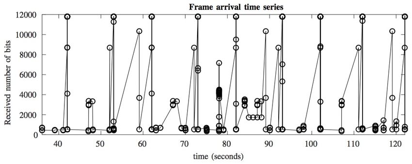
The next available observation time is The Lomb-Scargle method [21] generates a PSD estimate
min(s : s ≥ t, s ∈ T (x), if t ≤ max(T (x)),
of unevenly spaced time series, P : x n ∈ R 7→ x̂(ω) ∈ R+ ,
n(t) =:
+∞, (2) without the need to invent otherwise non-existent, evenly
otherwise. spaced data. The underpinning assumption is that the signals
For x ∈ T and t ∈ R, x(p(t)) is the previous observation are periodic. The approximate periodicity of unevenly spaced
value of x at time t, x(n(t)) is the next observation value of time series assumption is realistic when we consider the rate
x at t, and x l (t) = (1 − ω(t))x(p(t)) + ω(t)x(n(t)) where of arrival of audio or video frames during a streaming session
t−p(t)
(Fig. 2).
, if 0 < n(t) − p(t) < ∞ To reduce notation we subtract the mean from the signal x,
ω(t) =
n(t)−p(t)
0, (3)
otherwise, and then determine the normalized spectral content of x ∈ T
is the linearly interpolated value of x at time t. These acquisi- 2
n x n cos(ω(t n − τ))
P
1
x̂(ω) = P(x){ω} =
tion schemes are called last-observation, next-observation and ×
2σ 2 n cos (ω(t n − τ))
2
P
linear interpolation, respectively. We adopt the convention that
x(t) = x(n(t)) = x l (t) when t ∈ T (x). The interpolated signal
2
n x n sin(ω(t n − τ))
P
x l (t) is a continuous piece-wise-linear function. + (9)
n sin (ω(t n − τ))
P 2
Local-in-time statistics: It is convenient to consider short-
time observations of these time series in order to generate at the frequencies ω, where σ = N −1 n=1 (x n − µ) 2 . The
2 1 PN
local-in-time statistics of network behaviour. The time series following time offset is used to guarantee the time in-variance
generated in networks over a closed interval, which starts at of the computed spectrum
time s and ends at time t, [s, t], where s < t is PN
n=1 sin(2ωt n )
x{s, t} = ((t n, x n ) : s ≤ t n < t, 1 ≤ n ≤ N ). (4) tan(2ωτ) = P N . (10)
n=1 cos(2ωt n )
One acquisition approach (cf. [1]) is to apply the max We assume that network-generated time-series are base-
operator to the values in a closed interval [s, t] and to slide band or low-pass signals. Empirical evidence in Section VI
this interval, by some step-size, over the entire signal. The supports this assumption. To fix ideas, we stream a podcast
maximum signal value in the closed interval [s, t] is denoted from SoundCloud [14]. The average received bit-rate of the
as (t) = max V (x{s, t}) (5) podcast is 104, 991kbps. We capture an unevenly spaced
time series which consists of the time-stamps and sizes (in
The minimum value in this interval bits) of each frame, (t n, x n ) respectively, in the stream using
ms (t) = min V (x{s, t}) (6) TCPDUMP [22]. We filter out the time-stamp and frame sizes
and plot this unevenly spaced time series in Fig. 2. This trace
The average value in a closed interval is commonly used to has a periodic component – every approximately 10 seconds,
summarize system performance [5],[6] and [7]. a number of 12kbits frames are delivered.
p(t) In Fig. 3 we plot the PSD estimate of this unevenly spaced
1 X
time series. The component with the highest PSD is ≈ .7Hz.
µs (t) = xn (7)
|X {s, t}| n=n(s) By inspection of Fig. 2, we determine that the fundamental
frequency of this trace is < 1Hz. The upper envelope of the
The maximum, minimum and average statistics are reported PSD falls to 0dB/Hz at ≈ 100Hz. There are other higher-
by [20]. Other higher-order statistics are computed in a similar frequency components in Fig. 2. Consequently, in Fig. 3 we
manner, and may be of use to network monitoring applications. illustrate where the PSD of the trace has fallen by 50dB from
The time duration between consecutive observations of x is its peak value – this occurs at ≈ 108 Hz – to demonstrate a
useful for determining the rate of change of the time series range of frequencies of interest to monitoring applications.
∆t(x) = ((t n+1, t n+1 − t n ) : 1 ≤ n ≤ N − 1). (8) Do current time series acquisition approaches preserve this
important information about the rate of change and the period
III. ACQUIRE FASTER : P ERIODIC ACQUISITION of frame delivery? To answer this question, we acquire state
How representative are x(p(t)), x l (t) and µ x (t) of the data values every Ta = 1s, at times t ∈ N and examine the
they summarize? The acquisition methods used in [1], [2], [3] PSD of the resulting traces. The time period Ta = 1s is
and [4], are periodic, and use one of the approaches above, at representative of the period used in [1], [2], [3] and [4]. The
a rate of 1Hz or greater to quantify network behaviour. Given set of non-negative integers is N. The underlying process we
the increased dynamicity and complexity of modern networks want to acquire an accurate representation for, is acquired
this warrants further inspection. Is a periodic approach good by taking (1) the last sample closest to some sampling time,
enough? Is an acquisition rate of 1Hz appropriate? To de- x(p(t)) | t ∈ N; (2) the average value over the last sampling
termine the rate of change of unevenly spaced signals, we period, µt−1 (t) | t ∈ N \ 0, where t is in the set of
examine their spectral content by computing a Power Spectral positive integers; and finally, (3) the linear interpolated value
Density (PSD) estimate of x. x l (t) | t ∈ N. We use a stem to denote the position and height
102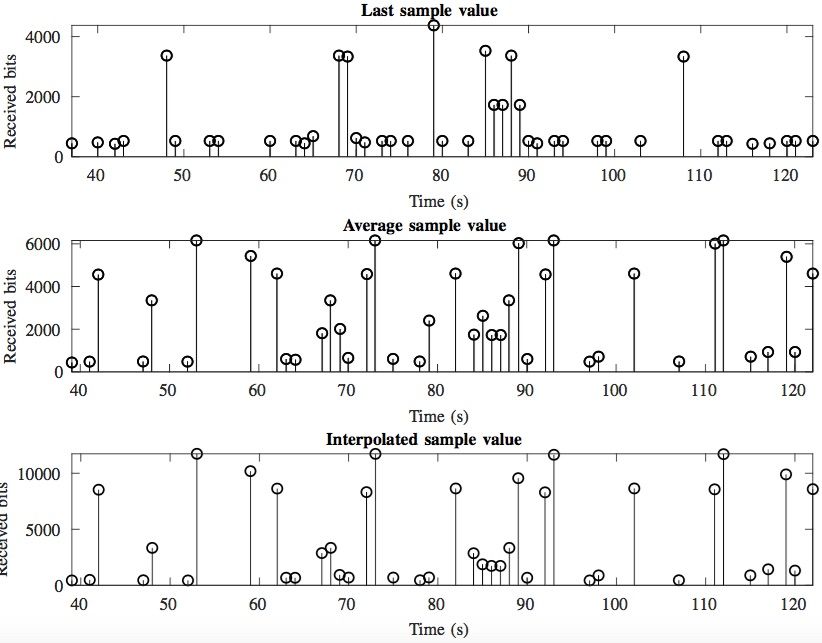
Fig. 2. Unevenly spaced time series observed when streaming audio to a
client. The time and value pairs illustrated consist of frame arrival time-stamps
and frame sizes. Every ≈ 10s a number of frames of size ≈ 12kbits are
received. This time-series has a clear periodic component.
Fig. 5. PSD of current acquisition approaches: x(p(t)), µt −1 (t) and xl (t).
Important information such as the rate of change of the underlying time
series and the period is lost. The flat PSDs illustrated demonstrate that higher
frequency information has been lost.
maximum rate of change of the network. The information in
Fig. 3. PSD of unevenly spaced time-series observed when receiving a the frequency band 0 < f < 108Hz is lost by the acquisition
streamed podcast from SoundCloud. The 50dB bandwidth is 108Hz. The methods used in Fig. 4. One reason for this is that they create
upper envelope of the PSD falls to 0dB at 100Hz. an estimate for data that does not exist.
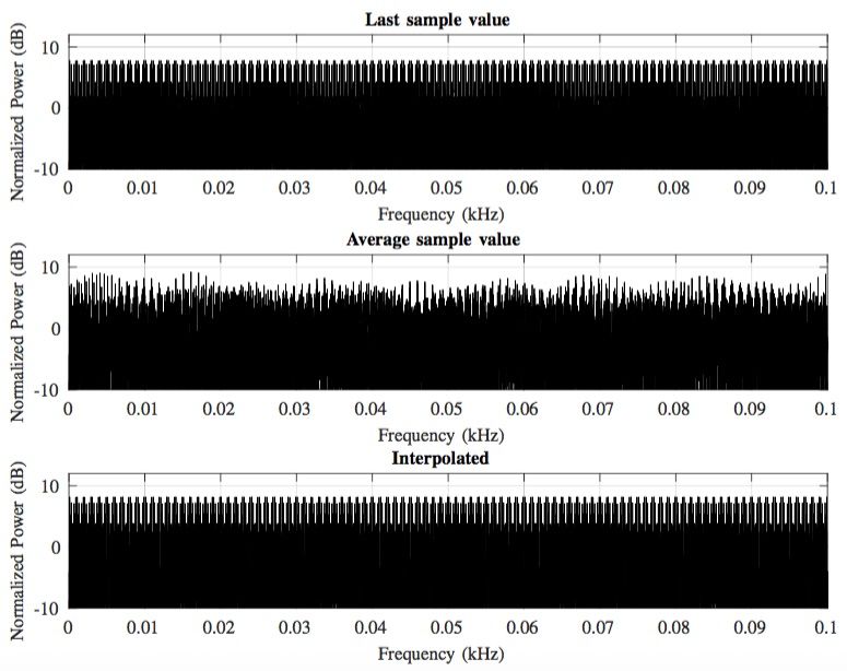
(1) Information about the period of the trace is lost.
This is a serious shortcoming. For example an artifact of
x(p(t)) is that its period is approximately 20 seconds and
not approximately 10 seconds. Period calculations for each
trace will be inaccurate as the times of frame arrivals in the
original trace are never in the set of times t ∈ N. For example
the 12kb frame arrival times occur just after 40, 50, 60, . . .
seconds. The large frame arrivals occur just before 50, 70, . . .
seconds in x(p(t)). In the average acquisition trace µt−1 (t),
the pulse amplitudes (frame sizes) vary in height, which makes
period detection hard. Finally the interpolated acquisition trace
x l (t) exhibits pulse amplitudes which vary each time they
appear with a period of 20 seconds. Estimates of the period
tell us when to expect the next burst of podcast data. The
ability to detect if this burst of data has arrived, or has arrived
late, is lost. This is because the exact times when bursts of
data arrive have been lost. Secondly, the sizes of the burst
have been lost; this is due to averaging or interpolation, or
Fig. 4. Using periodic acquisition (time-step of 1 second), we illustrate
the effect of using the last sample, average value and interpolated values
because the previous observation was not part of the periodic
at acquisition times t ∈ N. train of frames. The effect of using the last, average or
interpolated value over the previous second causes the period
information to be obscured. Averaging unevenly spaced time
of each state acquisition value in Fig. 4; each trace should be series introduces ambiguity.
compared with the original time series in Fig. 2. (2) Higher frequency information in the range up to
Analysis: The PSD allows us to estimate the rate of change of 108Hz and above is lost in Fig 5. The acquisition techniques,
the network/service – a parameter which is of crucial interest x(p(t)), µt−1 (t) and x l (t) low-pass filter the original unevenly
to service providers. For example, unusually high rates of spaced time-series. We posit that high-frequency variations
change may indicate anomalies; periodic components may in this trace may help us detect sub-optimal network per-
indicate that the network is healthy. The acquisition methods formance. Choosing a low-pass filter in the acquisition step,
in Fig. 4 do not allow the network manager to estimate the without reference to the rate of change of the time series, may
103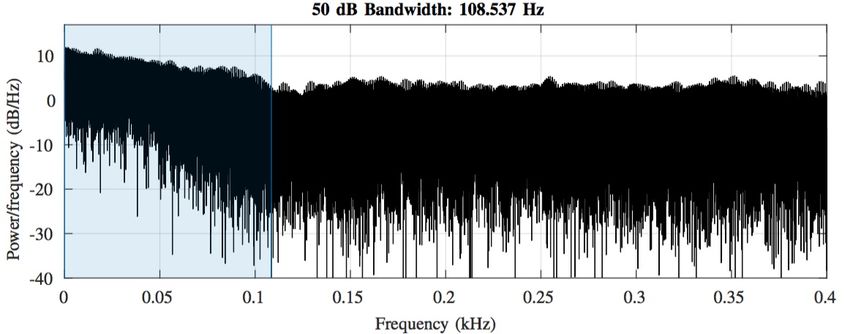
resulting rate of acquisition is unfeasibly high, knowledge
                                                                              of this parameter can facilitate better design decisions. For
                                                                              example, we can low-pass filter the signal and use this filtered
                                                                              time series in learning algorithms for example, cognizant of
                                                                              the fact that we cannot make predictions outside of a certain
                                                                              range of frequencies. We appeal to classical evenly spaced
                                                                              sampling theory for guidance with the challenge of rate of
                                                                              change estimation for unevenly spaced time series.
                                                                              The problem with unevenly spaced time series: The
                                                                              periodic time-series we observe for video and audio stream
                                                                              applications, x, consist of a sum of weighted and delayed Dirac
                                                                              pulses, δ(t), e.g.
                                                                                                     X N
                                                                                                          x(t n )δ(t − t n ).             (11)
                                                                                                      n=1

Fig. 6. High-rate periodic acquisition: Acquisition at 200 Hz does not        When these pulses form an infinitely long sequence of evenly
significantly improve the ability to estimate the period and rate of change   spaced pulses, spaced T seconds apart, and the pulses have
of the original data from the acquired time-series.                           identical heights, this is called a Dirac comb [23]. It is a known
                                                                              result in Signal Processing that the Fourier transform of a
                                                                              Dirac comb with period Ts produces another Dirac comb in
remove crucial monitoring and problem diagnosis information.
                                                                              the frequency domain with period T1 Hz. As these Dirac pulses
Remark: the amplitude and location in time of the acquired
                                                                              are spaced by T1 Hz in the frequency domain, to avoid aliasing,
stems (in Fig. 4) depend on the relative position of each
                                                                              we must ensure that the spectral content of the signal we wish
of the events in x relative to the acquisition times t ∈ N.
                                                                              to acquire is confined to a region of c = 2T     1
                                                                                                                                 Hz, which is
Shifting the acquisition times relative to the events in x, can
                                                                              the maximum permissible rate-of-change of this evenly spaced
greatly increase or decrease the efficacy of acquisition and
                                                                              time series.
monitoring. We have shown that for an arbitrary periodic
acquisition starting time that periodic acquisition is harmful                   Unlike the uniform case, the Fourier transform of the
for higher-order functions such as monitoring and learning.                   unevenly spaced time series in Eqn. 11 will generally not
   Higher acquisition rate: The periodic acquisition methods                  be a Dirac Comb, that is, a sequence of uniformly spaced
above, with a period of 1Hz, remove crucially important infor-                delta functions; the symmetry in the Dirac comb is broken
mation about the fundamental frequency and the rate of change                 by uneven spacing of the pulses, which leads to information
of frame delivery in Fig 2. Loss of this information will reduce              rich transform we observe in Fig. 3. This is because in the
the effectiveness of higher-order functions such as monitoring                Fourier domain, the locations and heights of the Dirac delta
and learning that consume the acquired performance data. The                  functions are related to the intervals between the time domain
PSD of the original unevenly spaced time-series experiences a                 observations. Randomizing the observation times, randomizes
drop of 50dB at approximately 100Hz in Fig. 3. We consider                    the locations and heights of the Fourier domain peaks and
the effect of acquiring this time series using a significantly                heights.
higher acquisition rate of 200Hz to determine if this facilitates                To leverage the results of classical sampling [23] to estimate
the capture of crucial parameters such as the period and rate                 c for an unevenly spaced time series, we express a unevenly
of change of the underlying trace. In effect we are assuming                  spaced time series as a evenly spaced time series. To this end,
that the Nyquist rate of this unevenly spaced time series is                  we determine the Dirac comb which has Dirac deltas that align
≈ 200Hz.                                                                      exactly with each of the pulses in the unevenly spaced time
   Increasing the rate of State Acquisition by a factor of                    series. In other words, we need to determine the largest Ta
200 increases the bandwidth of the monitoring protocol that                   such that each t n ∈ T (x) can be written as t n = α + nTa , for
consumes these metrics. Fig. 6 demonstrates that increasing                   integers n and an arbitrary time offset α.
the acquisition rate 200-fold does not improve our ability to                 Definition (1) Accurate acquisition: To accurately acquire an
estimate the period and rate of change of the time series. The                unevenly spaced time series the acquisition period Ta should
acquisition methods x(p(t)), µs (t) and x l (t) suffer to similar             satisfy the condition
problems as before; but they now consume more bandwidth
and storage.                                                                                  ∆t(x)    mod Ta = 0, ∀t n ∈ T N              (12)

              IV. R ATE OF C HANGE E STIMATION                                Definition (2) Rate-of-Change: The rate of change of the
   In this section we determine the appropriate way to acquire                unevenly spaced time series x is c = 2T1a if Ta satisfies the
periodic performance traces from audio and video streams by                   condition
estimating the rate of change, c, of the trace. Even if the                                  ∆t(x) mod Ta = 0, ∀t n ∈ T N              (13)

 104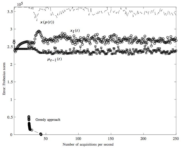
98.5% of the frame arrivals in this time-series. Averaging
                                                                            these values over a one-second interval, removes all frequency
                                                                            components above ≈ 1Hz, which make subsequent functions
                                                                            such as problem diagnosis difficult. Similarly in the case of
                                                                            fixed periodic acquisition rate of 1kHz (which is the time-step
                                                                            used by Prometheus [8]) this rate is too low for 94.25% of
                                                                            the frame arrivals in Fig. 2.
                                                                               From inspection of Fig. 7 it is clear that locally in time, the
                                                                            value of min ∆t(x) may be much higher than it would for the
Fig. 7. The time durations between consecutive frame arrivals ∆t (x) are    entire time series. This means that an acquisition performed at
plotted (stem height) on the LHS versus experiment time (x-axis). These     a rate that is consistent with the local rate of change of the time
durations are sorted from smallest to largest on the RHS. Very few of the   series, could be expected to significantly reduce the bandwidth
consecutive arrival times exhibit a large delay.
                                                                            required to accurately represent the underlying event steam
                                                                            x, over a periodic acquisition scheme with the same level
Finding the value of Ta that ensures that acquisition is being              of fidelity. We investigate an adaptive acquisition protocol,
performed at a sufficiently high rate, leads to acquisitions                where the value of Ta changes with time, and posit that it
rates which are impractical for real-world applications. If                 should give a more accurate time series representation, using
observation times are recorded to d decimal places, the largest             less bandwidth than before.
rate of change is determined by machine precision.                             A greedy approximation for the time series x is generated
   To make progress, we use a rough upper bound on Ta ,                     by summing a finite number of functions gi taken from a
which consists of examining the minimum separation between                  dictionary of such functions D. For example, the function g1
consecutive frame arrivals:                                                 consists of a sum of Diracs which are weighted by the largest
                                                                            value of the time series x, e.g. m1 = max(V (x)), which gives
                              min ∆t(x).                            (14)    the function                  X
As the traces we will consider are generally base-band signals,                                   g1 = m1      δ(t − t 1 (k))              (15)
we desire a value of Ta which captures most of the spectral                                                k

energy of the trace x.                                                      where t 1 is the set of times where x = m1 and there are k
Analysis: The smallest difference between two time-stamps,                  elements in this set.
min ∆t(x) in Fig. 2 is 10−7 seconds. This would necessitate ac-                The next function in the dictionary D is g2 . It consists of a
quiring the signal at an unfeasibly high rate, > 107 Hz, which              sum of Diracs which are weighted by the second largest value
is impractical most networking applications. We propose a                   of the time series x, m2 = max(V (x) \ m1 ). In words, we
Greedy Acquisition solution to solve this problem and examine               remove all of the instances of the maximum value of x from
a trade-off between the accuracy of the acquired time-series,               x and then find the next largest value, m2 . We then construct
the bandwidth of different versions of the acquired time-series.            the function g2 which has Dirac pulses of height m2 every
                                                                            time x = m2 ,
                    V. G REEDY ACQUISITION
                                                                                                       X
                                                                                               g2 = m2     δ(t − t 2 (k)).               (16)
   A Greedy Acquisition algorithm for unevenly spaced time-                                                k
series is presented that acquires observations at a rate which is           Similar to the previous case, t 2 is the set of times where x =
consistent with the rate of change of the original time series,             m2 ; there are k elements in this set. Continuing this process,
c.                                                                          we construct the entire dictionary D = {gi }.
   Fig. 7 demonstrates the number of time intervals between                   A j-th order approximation of x, which is denoted y j , is
consecutive values in x (the audio trace) that are greater than             obtained by summing up the first j elements of the dictionary
1 second (on the RHS). In summary, only 1.5% of these
                                                                                                                j
time intervals are greater than 1s; the majority of the time                                                    X
                                                                                                       y j :=         gi .                 (17)
spacings between events are much smaller. A useful rule of
                                                                                                                i=1
thumb for periodic acquisition is that if we increase the time
between acquisitions in the acquisition routine, we decrease                The accuracy of the jth order approximation is computed using
the range of frequencies that we can observe in the trace                   the Frobenius norm,
                                                                                                      s
[23]. It is challenging to perform accurate acquisition using
a periodic acquisition scheme because the time-step must be                                     j =       (x − y j ) 2 dt,          (18)
sufficiently small to capture a range of rates of change. Using
a fixed, periodic acquisition rate which is of the order of                 where y j (t n ) = 0 if we have not acquired a value at time t = t n
1Hz (in [5] and [7]) or even one kilohertz (in [6]) will not                for the jth approximation.
yield an accurate representation of the performance of x. For                  The set of values m1, m2, . . . are the values of the frame
example, for the audio streaming trace in Fig. 2, an acquisition            sizes sorted from largest to smallest. Because these frames
rate of 1Hz is significantly too low an acquisition rate for                are generated as part of well-defined protocols, which have

                                                                                                                                            105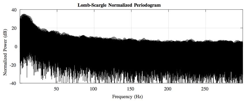
Data: input: real-time process for acquisition from x and
            β.
   Result: acquired time series (t n, yn ).
   initialization: sorted list of frame sizes mi from historical
    data;
   while still receiving stream do
        read current value;
        if x > β then
            acquire time t n = t;
            acquire the value yn = x n ;
        else
            do not acquire value or time;
        end
   end
     Algorithm 1: Online Greedy Acquisition Algorithm

                                                                               Fig. 9. Comparison of the acquisition accuracy bandwidth trade-off achieved
                                                                               using tradition periodic acquisition methods (last observation, average and
                                                                               interpolation) and using Greedy Acquisition. The greedy approach is signifi-
                                                                               cantly better.

                                                                               the approximation of x. (2) The bandwidth requirement of
                                                                               greedy approximation increases as j increases, but it increases
                                                                               efficiently, in line with the rate-of-change of x. (3) Because the
                                                                               original frame arrival times are used, the periodic component
                                                                               of the time series is generally captured by (t n, yn ); moreover,
                                                                               the rate-of-change of the time-series (t n, yn ) is generally
                                                                               consistent with that of (t n, x n ), in comparison with a periodic
                                                                               acquisition algorithm, which chooses the acquisition period in
                                                                               an arbitrary way, and is thus, not always suited to the process
                                                                               being observed.
Fig. 8. Frame arrival process statistic acquisition for the SoundCloud trace                     VI. N UMERICAL E VALUATION
using Greedy Acquisition: The error in the acquisition time-series decreases
as the number of acquisitions per second increases. We examine the first          We examine the accuracy of different acquisition methods
through to the sixtieth order approximation of x. The error achieved when 25   using a simple video and audio use-case. We focus on audio
measurements are acquired on average per second is impressively low, given
that we are computing the Frobenius norm of frame sizes of up to 12kbits.      and video because according to Cisco, by 2021, 82% of all
                                                                               consumer Internet traffic will be IP video traffic [24]. The
                                                                               ability to acquire measurements from the traces clients receive
predetermined frame sizes for an array of scenarios, the                       will be crucial. Higher quality acquisition data will improve
number of different values of mi that we can expect is finite,                 next-generation monitoring protocols.
and generally, quite small. It is possible to determine the set                   Our hypothesis is that Greedy Acquisition yields more
{mi }i a-priori for any given service.                                         accurate estimates of the observed process than traditional pe-
   An online real-time version of the Greedy Acquisition                       riodic monitoring approaches. Moreover, we posit that Greedy
algorithm presented above, is presented in Alg. 1. It consists                 Acquisition uses less bandwidth and storage, and that the
of determining whether or not the current frame arrival has                    acquired time-series preserve important statistical features of
a frame size which is larger than a user defined threshold,                    the observed trace, such as its period. In our comparison we
β. The value of β determines the accuracy of the achieved                      implement acquisition functions which estimate x(p(t)), µs (t)
approximation. If an incoming frame size is larger than β, the                 and x l (t). The reason that we do not use off-the-shelf tools
frame size and time are recorded as part of the unevenly spaced                such as SAR [5] is that they have a minimum acquisition
acquired time series (t n, yn ). Greedy approximation has the                  rate of 1Hz (in the case of SAR), a rate which we would
following properties. (1) the accuracy of the approximation                    like to significantly increase, in order to fully evaluate the
increases monotonically as β decreases, because each increase                  potential of periodic acquisition. We consider a frame arrival
in the order of the approximation j, reduces the error in                      process because TCPDUMP [22] provides easy access to high

 106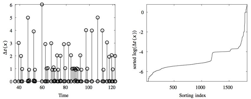
resolution time-stamps for a widely available unevenly spaced
time series, which is representative of what we might observe
at many other intermediate points in the network.
   Experimental set-up: In the first scenario a client streams
a podcast from an online audio distribution platform, a Sound-
Cloud instance [14]. In 2014 SoundCloud boasted 75 million
unique monthly listeners, which demonstrates the popularity
of the service, and motivates the need to be able to accurately
acquire measurements from the audio traces. In the second
scenario a client streams a video from a video server of an
Irish public service broadcaster [25].                                  Fig. 10. PSD of frame arrival time series for video streaming session. This
   During our evaluation of both scenarios, the client requested        trace has a periodic component at 5.4Hz, which implies that acquiring this
                                                                        trace at 1Hz is insufficient.
the service and then TCPDUMP [22] was used to capture
a description of the contents of the frames received on the
client’s network interface. Once the media session had ter-             on their importance (frame size).
minated, we converted the captured .pcap file to text format               The traditional periodic approaches have time steps in the
using tshark, and we greped the resulting text file for the frame       range 1/ps where p = 1 . . . 250Hz in these experiments. These
arrival times, t n , and frame sizes x n , forming the unevenly         periodic approaches cannot observe the fastest changes in the
spaced time series (t n, x n ). Frame arrival times were captured       observed process, or at the maximum rate of change of the
in terms of hours, minutes, seconds, and fractions of a second          process. In conclusion, periodic acquisition approaches yield
since midnight. We recorded the size of received frames using           an error which is 5 times worse than the error of Greedy
the “bytes on wire” field, in bits. We stored frame arrival             Acquisition, using 5 times the bandwidth to do so. Finally,
times using double-precision according to IEEE Standard 754             important statistics of the observed traces are typically not
for double precision, which bounded the precision of rate-of-           preserved by periodic approaches.
change estimates. The frame sizes were integer-valued. For                 In the case of the video streaming session, we illustrate the
the SoundCloud session, the maximum frame received was                  PSD of the time-series in order to provide initial estimates
11792 bits, and 60 different frame sizes were observed during           for the period and the rate-of-change of x. This trace has a
this session, which gave us 60 different potential acquisition          periodic component at 5.4Hz, which implies that acquiring
accuracies. In all cases we streamed data for ≈ 15 minutes.             this trace using a periodic acquisition method at 1Hz is insuf-
   Discussion: Fig. 8 illustrates the error (Eqn. 18) versus            ficiently accurate. Note that even the recommended reporting
bandwidth trade-off achieved for a SoundCloud session by                rate of RTCP (5Hz) is not sufficiently large to capture the
varying β in the online Greedy Acquisition algorithm. As                period of this trace. In addition, the PSD of this trace exhibits
the value of β is decreased, the accuracy of the greedy                 significant power up to 100Hz. Similar to the audio streaming
representation improves. This accuracy comes at the cost of             scenario, increasing the acquisition rate of periodic acquisition
25 acquisitions per second on average.                                  algorithms does not significantly improve the accuracy of the
   This result is significant, particularly when it is compared         acquired time series.
with the periodic, last-observation, averaging and interpolation           With regard to the rate of change of this trace, 0.16% of
schemes currently used (x(p(t)), µs (t) and x l (t)). Fig. 9            consecutive frame arrivals have an inter-arrival time of greater
illustrates the accuracy of x(p(t)), µs (t) and x l (t) as a function   than 1s, and 1.3% have an inter-arrival time of greater than
of the bandwidth consumed by these acquisition approaches.              10−3 s. The minimum inter-arrival time is less than 10−7 s.
The bandwidth is increased by increasing the resolution of the          Given the definition of the rate of change of unevenly spaced
acquisition time-step. For the periodic acquisition methods,            times series, periodic acquisition at 1Hz is insufficient.
the trend is for the error to decrease as the rate of acquisition          These statistics underline the difficulty of choosing a time-
increases. We increase the rate of acquisition from 1Hz up to           step for periodic acquisition that would yield sufficiently high
250Hz in steps of 1Hz.                                                  accuracy. We evaluate Greedy Acquisition, to see if acquiring
   In this trace the times of the arrivals of the largest frame         measurements at a rate which is consistent with the rate of
sizes tend to determine the periodic component of the time              change of the trace, is accurate. Fig. 11 demonstrates that
series. Preserving the exact times of events is important. The          accurate acquisition is achieved by taking 300 acquisitions per
ability to so, is determined by the rate of acquisition. The            second using Greedy Acquisition. The average acquisition rate
Greedy Acquisition algorithm acquires a trace at a rate which           for video that achieves the same accuracy as audio acquisition
is consistent with the rate of change of time series. For               is approximately ×10 the acquisition rate for audio. Once
the 1st approximation y1 , the minimum time-step between                again Greedy Acquisition out-performs each of the periodic
consecutive frame arrivals min ∆t(y1 ) does not change as we            acquisition approaches – by an order of magnitude drop in
increase the order of the approximation. The 1st approximation          the error of the representation – when 300 acquisitions are
y1 , and all subsequent approximations have the possibility of          made per second.
capturing the fastest changes in the observed trace, depending             Recommendations: Many current periodic acquisition ap-

                                                                                                                                               107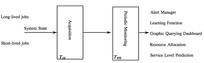
present-day acquisition techniques do not capture information
                                                                                   which is crucially important for problem diagnosis. Our exper-
                                                                                   iments with real-world voice and video traces demonstrate that
                                                                                   high quality State Acquisition is possible if the time-stamps
                                                                                   and magnitudes of events are recorded at the rate of change
                                                                                   of the application.
                                                                                                                  R EFERENCES
                                                                                    [1] D. Jurca and R. Stadler, “H-GAP: estimating histograms of local
                                                                                         variables with accuracy objectives for distributed real-time monitoring,”
                                                                                         IEEE Trans. Net. and Serv. Man., vol. 7, no. 2, pp. 83–95, Jun. 2010.
                                                                                    [2] R. Yanggratoke, J. Ahmed, J. Ardelius, C. Flinta, A. Johnsson, D. Gill-
                                                                                         blad, and R. Stadler, “Predicting real-time service-level metrics from
                                                                                         device statistics,” IFIP/IEEE Int. Sym. Int. Net. Man., pp. 1–8, 2015.
                                                                                    [3] R. de Fréin, “Source separation approach to video quality prediction in
                                                                                         computer networks,” IEEE Comm Ltr, vol. 20, no. 7, pp. 1333–1336,
                                                                                         Jul. 2016.
                                                                                    [4] R. Mijumbi, S. Hasija, S. Davy, A. Davy, B. Jennings, and R. Boutaba,
                                                                                         “Topology-aware prediction of virtual network function resource require-
Fig. 11. Frame arrival process statistic acquisition for video trace using               ments,” IEEE Trans Net. Serv. Man., vol. 14, no. 1, pp. 106–120, 2017.
Greedy Acquisition: The error in the acquisition time series decreases as           [5] S. Godard, “SAR,” http://linux.die.net/man/1/sar.
the number of acquisitions per second increases. The error achieved when            [6] E. Galstad. (1999) Nagios. [Online]. Available: https://www.nagios.com/
300 measurements are acquired on average per second is impressively low.            [7] R. Binns. top. [Online]. Available: https://linux.die.net/man/1/top
The periodic acquisition methods x(p(t)), µ−1 (t) and xl (t) are illustrated for    [8] J.        Volz       and      B.       Rabenstein.        (2018)     Sound
completeness.                                                                            Cloud       Developers:      Backstage       Blog.     [Online].     Avail-
                                                                                         able: https://developers.soundcloud.com/blog/prometheus-monitoring-
                                                                                         at-soundcloud
                                                                                    [9] ETSY. StatsD. [Online]. Available: https://github.com/etsy/statsd
proaches acquire time-series without knowledge of the under-                       [10] R. de Fréin, C. Olariu, Y. Song, R. Brennan, P. McDonagh, A. Hava,
lying rate of change of the time series under observation.                               C. Thorpe, J. Murphy, L. Murphy, and P. French, “Integration of QoS
                                                                                         Metrics, Rules and Semantic Uplift for Advanced IPTV Monitoring,” J.
We have argued that knowledge of the rate of change of                                   Net. Sys. Man., vol. 23, no. 3, pp. 673–708, Jul 2015.
the process under observation, should drive the process of                         [11] R. de Fréin, “The data-centre whisperer: Relative attribute usage esti-
deciding when to acquire measurements of this process. Many                              mation for cloud servers,” in 24th EUSIPCO, Aug. 2016, pp. 687–691.
                                                                                   [12] Q. Zhang, L. Cheng, and R. Boutaba, “Cloud computing: state-of-the-
networking time-series exhibit properties such as periodicity.                           art and research challenges,” J. of Int. Serv. and Apps, vol. 1, no. 1, pp.
These properties should be preserved by acquisition routines.                            7–18, May 2010.
One point of note from this work is that the times of events                       [13] D. Josephsen, Building a Monitoring Infrastructure with Nagios. Upper
                                                                                         Saddle River, NJ, USA: Prentice Hall PTR, 2007.
T (x) are as important as the values recorded for these events                     [14] A. Ljung and E. Wahlforss. (2008) SoundCloud. [Online]. Available:
V (x). Periodic acquisition routines such as Nagios, record                              https://soundcloud.com/
values with greater precision than times, due the default time                     [15] R. de Fréin, “Effect of system load on video service metrics,” in IEEE
                                                                                         Irish Sig. Sys. Conf. (ISSC), 2015, pp. 1–6.
resolution of 10−3 s. A second point of note is that the wide                      [16] “The Cacti Group Inc.” [Noline], 2016, accessed on Dec. 28, 2016.
array of off-the-shelf acquisition routines means that little                            [Online]. Available: http://www.cacti.net/
research is being done in the area. The received wisdom is that                    [17] V. Jacobson, R. Frederick, S. Casner, and H. Schulzrinne, “RTP: A
                                                                                         transport protocol for real-time applications,” IETF RFC3550, 2003.
metric acquisition routines exist, and thus, there is little point                       [Online]. Available: https://tools.ietf.org/html/rfc3550
in re-inventing them. Finally, we have provided evidence that                      [18] A. Begen, T. Akgul, and M. Baugher, “Watching video over the web:
Greedy Acquisition gives improved acquisition performance.                               Part 1: Streaming protocols,” IEEE Int. Comp., vol. 15, no. 2, pp. 54–63,
                                                                                         Mar. 2011.
                                                                                   [19] ——, “Watching video over the web: Part 2: Applications, standard-
                          VII. C ONCLUSIONS                                              ization, and open issues,” IEEE Int. Comp., vol. 15, no. 3, pp. 59–63,
                                                                                         2011.
   In this paper we showed that acquiring a system or service’s                    [20] “Datadog,” Online documentation, accessed on Dec. 28, 2016. [Online].
state at a rate which was consistent with the rate of change                             Available: https://www.datadoghq.com/
                                                                                   [21] N. R. Lomb, “Least-squares frequency analysis of unequally spaced
of the system (or service) provided a high-quality record of                             data,” Astrophy. and Space Sc., vol. 39, no. 2, pp. 447–462, Feb. 1976.
the state of the system. Research on capturing system state has                    [22] V. Jacobson, C. Leres, and S. McCanne. tcpdump. [Online]. Available:
lagged behind the growth of networks and the applications that                           http://www.tcpdump.org/
                                                                                   [23] M. Vetterli, J. Kovacevic, and V. K. Goyal, Foundations of Signal
use these networks as a substrate. Today, many monitoring and                            Processing. Cambridge: Cambridge Univ. Press, 2014.
learning solutions rely on standard periodic State Acquisition                     [24] “Cisco         Visual      Networking         Index:       Forecast     and
solutions, which acquire the system state at a frequency of                              Methodology,            2016-2021.”            [Online].         Available:
                                                                                         https://www.cisco.com/c/en/us/solutions/collateral/service-
1Hz. These solutions do not capture important characteristics                            provider/visual-networking-index-vni/complete-white-paper-c11-
of the signals they acquire, for example, periodicity and rate of                        481360.html
change. For periodic traces, the ability to estimate the period                    [25] (1996)         TG4:       TG       Ceathair.       [Online].      Available:
                                                                                         http://www.tg4.ie/en/player/home/
from an acquired representation of the trace is fundamental.
                                                                                   This publication has emanated from research conducted with the finan-
We demonstrated that the rate of change of many applications                       cial support of Science Foundation Ireland (SFI) under the Grant Number
is much greater than 1 Hz, and then, we demonstrated that                          15/SIRG/3459.

 108
You can also read