Auto-Directed Video Stabilization with Robust L1 Optimal Camera Paths
←
→
Page content transcription
If your browser does not render page correctly, please read the page content below
Auto-Directed Video Stabilization with Robust L1 Optimal Camera Paths

                        Matthias Grundmann1,2             Vivek Kwatra1                      Irfan Essa2
                       grundman@cc.gatech.edu          kwatra@google.com               irfan@cc.gatech.edu
                1                                                 2
                    Google Research, Mountain View, CA, USA           Georgia Institute of Technology, Atlanta, GA, USA

                           Abstract                                     smooth camera path, and (3) Synthesizing the stabilized
                                                                        video using the estimated smooth camera path.
    We present a novel algorithm for automatically applying                 We address all of the above steps in our work. Our key
constrainable, L1-optimal camera paths to generate stabi-               contribution is a novel algorithm to compute the optimal
lized videos by removing undesired motions. Our goal is to              steady camera path. We propose to move a crop window
compute camera paths that are composed of constant, lin-                of fixed aspect ratio along this path; a path optimized to
ear and parabolic segments mimicking the camera motions                 include salient points and regions, while minimizing an L1-
employed by professional cinematographers. To this end,                 smoothness constraint based on cinematography principles.
our algorithm is based on a linear programming framework                Our technique finds optimal partitions of smooth paths by
to minimize the first, second, and third derivatives of the re-         breaking the path into segments of either constant, linear, or
sulting camera path. Our method allows for video stabiliza-             parabolic motion. It avoids the superposition of these three
tion beyond the conventional filtering of camera paths that             types, resulting in, for instance, a path that is truly static
only suppresses high frequency jitter. We incorporate addi-             within a constant segment instead of having small residual
tional constraints on the path of the camera directly in our            motions. Furthermore, it removes low-frequency bounces,
algorithm, allowing for stabilized and retargeted videos.               e.g. those originating from a person walking with a camera.
Our approach accomplishes this without the need of user                 We pose our optimization as a Linear Program (LP) subject
interaction or costly 3D reconstruction of the scene, and               to various constraints, such as inclusion of the crop window
works as a post-process for videos from any camera or from              within the frame rectangle at all times. Consequently, we
an online source.                                                       do not perform additional motion inpainting [10, 3], which
                                                                        is potentially subject to artifacts.
1. Introduction
                                                                        Related work: Current stabilization approaches employ
Video stabilization seeks to create stable versions of casu-            key-point feature tracking and linear motion estimation in
ally shot video, ideally relying on cinematography princi-              the form of 2D transformations, or use Structure from Mo-
ples. A casually shot video is usually filmed on a handheld             tion (SfM) to estimate the original camera path. From this
device, such as a mobile phone or a portable camcorder                  original shaky camera path, a new smooth camera path is es-
with very little stabilization equipment. By contrast, pro-             timated by either smoothing the linear motion models [10]
fessional cinematographers employ a wide variety of sta-                to suppress high frequency jitter, or fitting linear camera
bilization tools, such as tripods, camera dollies and steady-           paths [3] augmented with smooth changes in velocity to
cams. Most optical stabilization systems only dampen high-              avoid sudden jerks. If SfM is used to estimate the 3D path
frequency jitter and are unable to remove low-frequency                 of the camera, more sophisticated smoothing and linear fits
distortions that occur during handheld panning shots, or                for the 3D motion may be employed [8].
videos shot by a walking person. To overcome this limita-                   To rerender the original video as if it had been shot from
tion, we propose an algorithm that produces stable versions             a smooth camera path, one of the simplest and most robust
of videos by removing undesired motions. Our algorithm                  approaches is to designate a virtual crop window of pre-
works as a post process and can be applied to videos from               defined scale. The update transform between the original
any camera or from an online source without any knowl-                  camera path and the smooth camera path is applied to the
edge of the capturing device or the scene.                              crop window, casting the video as if it would have been shot
    In general, post-process video stabilization [10] consists          from the smooth camera path. If the crop window does not
of the following three main steps: (1) Estimating the origi-            fit within the original frame, undefined out-of-bound areas
nal (potentially shaky) camera path, (2) Estimating a new               may be visible, requiring motion-inpainting [3, 10]. Addi-

                                                                  225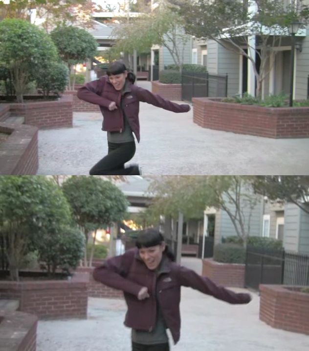
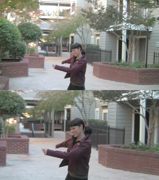
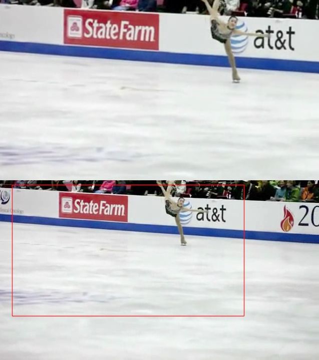
Figure 1: Five stills from our video stabilization with saliency constraints using a face detector. Original frames on top, our face-directed
final result at the bottom. The resulting optimal path is essentially static in y (the up and down motion of camera is completely eliminated)
and composed of linear and parabolic segments in x. Our path centers the object of interest (jumping girl) in the middle of the crop window
(bottom row) without sacrificing smoothness of the path. Please see accompanying video.

tionally, image-based rendering techniques [1] or light-field                We want our computed camera path P (t) to adhere to
rendering (if the video was captured by a camera array [13])              these cinematographic characteristics, but choose not to in-
can be used to recast the original video.                                 troduce additional cuts beyond the ones already contained
    While sophisticated methods for 3D camera stabiliza-                  in the original video. To mimic professional footage, we
tion [8] have been recently proposed, the question of how                 optimize our paths to be composed of the following path
the optimal camera path is computed is deferred to the user,              segments:
either by designing the optimal path by hand or selecting                    • A constant path, representing a static camera,
a single motion model for the whole video (fixed, linear or                    i.e. DP (t) = 0, D being the differential operator.
quadratic), which is then fit to the original path. The work                 • A path of constant velocity, representing a panning or
of Gleicher and Liu [3] was the first to our knowledge to                      a dolly shot, i.e. D2 P (t) = 0.
use a cinematography-inspired optimization criteria. Beau-                   • A path of constant acceleration, representing the ease-
tifully motivated, the authors propose a system that creates                   in and out transition between static and panning cam-
a camera path using greedy key-frame insertion (based on                       eras, i.e. D3 P (t) = 0.
                                                                          To obtain the optimal path composed of distinct constant,
a penalty term), with linear interpolation in-between. Their
                                                                          linear and parabolic segments, instead of a superposition of
system supports post-process saliency constraints. Our al-
                                                                          them, we cast our optimization as a constrained L1 min-
gorithm approximates the input path by multiple, sparse
                                                                          imization problem. L1 optimization has the property that
motion models in one unified optimization framework in-
                                                                          the resulting solution is sparse, i.e. it will attempt to sat-
cluding saliency, blur and crop window constraints. Re-
                                                                          isfy many of the above properties along the path exactly.
cently, Liu et al. [9] introduced a technique that imposes
                                                                          The computed path therefore has derivatives which are ex-
subspace constraints [5] on feature trajectories when com-
                                                                          actly zero for most segments. On the other hand, L2 min-
puting the smooth paths. However, their method requires
                                                                          imization will satisfy the above properties on average (in
long feature tracks over multiple frames.
                                                                          a least-squared sense), which results in small but non-zero
    Our proposed optimization is related to L1 trend filtering            gradients. Qualitatively, the L2 optimized camera path al-
[6], which obtains a least square fit, while minimizing the               ways has some small non-zero motion (most likely in the
second derivate in L1 norm, therefore approximating a set                 direction of the camera shake), while our L1 optimized path
of points with linear path segments. However, our algorithm               is only composed of segments resembling a static camera,
is more general, as we also allow for constant and parabolic              (uniform) linear motion, and constant acceleration.
paths (via minimizing the first and third derivate). Figure 8                Our goal is to find a camera path P (t) minimizing the
shows that we can achieve L1 trend filtering through a par-               above objectives while satisfying specific constraints. We
ticular weighting for our objective.                                      explore a variety of constraints:
                                                                          Inclusion constraint: A crop window transformed by the
2. L1 Optimal Camera Paths                                                     path P (t) should always be contained within the frame
                                                                               rectangle transformed by C(t), the original camera
From a cinematographic standpoint, the most pleasant                           path. When modeled as a hard constraint, this allows
viewing experience is conveyed by the use of either static                     us to perform video stabilization and retargeting while
cameras, panning ones mounted on tripods or cameras                            guaranteeing that all pixels within the crop window
placed onto a dolly. Changes between these shot types can                      contain valid information.
be obtained by the introduction of a cut or jerk-free transi-             Proximity constraint: The new camera path P (t) should
tions, i.e. avoiding sudden changes in acceleration.                           preserve the original intent of the movie. For example,

                                                                    226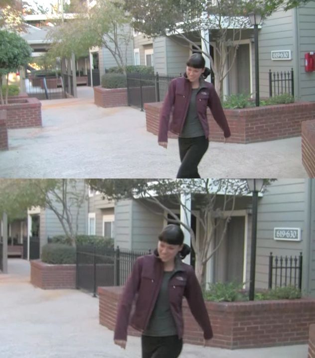
if the original path contained segments with the camera
                                                                             Residual
     zooming in, the optimal path should also follow this                    motion
                                                                                                        R1                    R2

     motion, but in a smooth manner.                                                     B1 = C-11 P1          B2 = C-12 P2          B3 = C-13 P3
                                                                             Crop
Saliency constraint: Salient points (e.g. obtained by a face                 window

     detector or general mode finding in a saliency map)                     Camera                     F2                    F3
                                                                             path Ct
     should be included within all or a specific part of the                 (known)
     crop window transformed by P (t). It is advantageous
                                                                                             C1                    C2                   C3
     to model this as a soft constraint to prevent tracking
     of salient points, which in general leads to non-smooth               Figure 2: Camera path. We seek to find the update trans-
     motion of the non-salient regions.                                    form Bt for each frame, such that the L1 norm of the residual
2.1. Solution via Linear Programming                                       |Rt | = |Ft+1 Bt+1 − Ft | is minimized for all t (static camera). By
                                                                           minimizing the difference of the residuals |Rt+1 − Rt | as well, we
For the following discussion we assume that the camera                     can achieve a path that is composed of static and linear segments
path C(t) of the original video footage has been computed                  only. Refer to text for parabolic segments.
(e.g. from feature tracks) and is described by a parametric
linear motion model at each instance of time. Specifically,                over all Bt 1 . In fig. 2 we visualize the intuition behind this
let the video be a sequence of images I1 , I2 , . . . , In , where         residual. A constant path is achieved when applying the
each frame pair (It−1 , It ) is associated with a linear motion            update transform B2 and feature transform F2 in succession
model Ft (x) modeling the motion of feature points x from                  to frame I2 yields the same result as applying B1 to frame
It to It−1 . From now on, we will consider the discretized                 I1 , i.e. R1 = 0.
camera path Ct defined at each frame It . Ct is iteratively                2. Minimizing |D2 (P )|1 : P          While forward differenc-
computed by the matrix multiplication                                                        2
                                                                           ing
                                                                           P       gives  |D   (P )|      =       t |DPt+2 − DPt+1 |     =
                                                                               t |P t+2 − 2P t+1  +  P t |, care  has to be  taken, as  we
          Ct+1 = Ct Ft+1 =⇒ Ct = F1 F2 ...Ft .                (1)
                                                                           model the error as additive instead of compositional. We
While we focus our discussion on 2D parametric motion                      therefore minimize directly the difference of the residuals
models Ft , our system is theoretically applicable to higher
dimensional linear motions though we do not explore them
in this paper.                                                               |Rt+1 − Rt | = |Ft+2 Bt+2 − (I + Ft+1 )Bt+1 + Bt | (5)
    Given the original path Ct , we express the desired                    as indicated in fig. 2.
smooth path as                                                             3. Minimizing |D3 (P )|1 : Similarly,
                       Pt = Ct Bt ,                      (2)
where Bt = Ct−1 Pt is the update transform that when ap-                   |Rt+2 − 2Rt+1 + Rt | =                                                   (6)
plied to the original camera path Ct , yields the optimal path             |Ft+3 Bt+3 − (I + 2Ft+2 )Bt+2 + (2I + Ft+1 )Bt+1 − Bt |.
Pt . It can be interpreted as the “stabilization and retargeting
transform” (or crop transform) which is applied to the crop                4. Minimizing over Bt : As initially mentioned, the known
window centered at each frame to obtain the final stabilized               frame-pair transforms Ft and the unknown update trans-
video. The optimization serves to find the optimal stable                  forms Bt are represented by linear motion models. For ex-
camera path P (t) minimizing the objective                                 ample, Ft may be expressed as 6 DOF affine transformation

  O(P ) = w1 |D(P )|1 + w2 |D2 (P )|1 + w3 |D3 (P )|1 (3)                                           at bt       x1       dxt
                                                                                  Ft = A(x; pt ) =                   +
                                                                                                     ct dt      x2       dyt
subject to multiple previously mentioned constraints. With-
out constraints, the optimal path is constant: Pt = I, ∀t.                 with pt being the parametrization vector pt                  =
                                                                           (dxt , dyt , at , bt , ct , dt )T . Similar a 4 DOF linear sim-
1. MinimizingP |D(P )|1 : Using P forward differencing;
|D(P )| = t |Pt+1 − Pt | = t |Ct+1 Bt+1 − Ct Bt | us-                      ilarity is obtained by setting at = dt and bt = −ct .
ing eq. (2). Applying the decomposition of Ct in eq. (1)                      We seek to minimize the weighted L1 norm of the resid-
                      X                                                    uals derived in eqs. (4) to (6) over all update transforms Bt
            |D(P )| =     |Ct Ft+1 Bt+1 − Ct Bt |                          parametrized by their corresponding vector pt . Then, the
                         t                                                 residual for the constant path segment in eq. (4) becomes
                         X
                     ≤       |Ct ||Ft+1 Bt+1 − Bt |.
                         t
                                                                                           |Rt (p)| = |M (Ft+1 )pt+1 − pt |,
                                                                              1 Note,
With Ct known, we therefore seek to minimize the residual                              that we chose an additive error here instead of the composi-
         X                                                                 tional error min |St | s.t. Ft+1 Bt+1 − Bt St = 0, which is better suited
            |Rt |, with Rt := Ft+1 Bt+1 − Bt          (4)                  for transformations, but quadratic in the unknowns and requires a costlier
             t
                                                                           solver than LP.

                                                                     227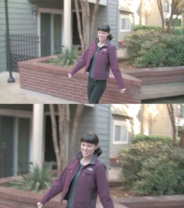
Motion in x over frames Motion in y over frames
where M (Ft+1 ) is a linear operation representing the ma- original path original path
300 optimal L1 path 300 optimal L1 path
trix multiplication of Ft+1 Bt+1 in parameter form.
5. The LP minimizing the L1 norm of the residuals (eqs. (4) 200
Frames
200
Frames
to (6)) in parametric form can be obtained by the introduc-
tion of slack variables. Each residual will require the in- 100 100
troduction of N slack variables, where N is the dimension
0 0
of the underlying parametrization, e.g. N = 6 in the affine −100 0 100
Motion in x
200 −40 −20 0
Motion in y
20 40
case. For n frames this corresponds to the introduction of
roughly 3nN slack variables. Specifically, with e being a Figure 4: Optimal camera path obtained via our constrained LP
vector of N positive slack variables, we bound each resid- formulation for the video in fig. 10. Shown is the motion in x and
ual from below and above e.g. for |D(P )|: y over a period of 320 frames, using the inclusion constraint for a
crop window of 75% size of the original frame. Note how the op-
−e ≤ M (Ft+1 )pt+1 − pt ≤ e timal path is composed of constant, linear and parabolic arcs. Our
method is able to replace the low-frequency bounce in y (person
with e ≥ 0. The objective is to minimize cT e which cor- walking with a camera) with a static camera while guaranteeing
responds to the minimization of the L1 norm if c = 1. that all pixels within the crop window are valid.
By adjusting the weights of c we can steer the minimiza-
tion towards specific parameters, e.g. we can weight the The complete L1 Frame rectangle [0, w] x [0,h]
strictly affine part higher than the translational part. This is minimization LP for Corners
also necessary as translational and affine parts have differ- the optimal camera ci trans-
formed Crop
ent scales, we therefore use a weighting of 100:1 for affine path with constraints
recta
ngle
by A(pt)
to translational parts. is summarized in
Using the LP formulation of our problem, it easy to im- Algorithm 1. We show
pose constraints on the optimal camera path. Recall, that pt Figure 3: Inclusion constraint.
an example of our
represents the parametrization of the update transform Bt , computed optimal path from the original camera path in
which transforms a crop window originally centered in the fig. 4. Note how the low-frequency bounce in y, originating
frame rectangle. In general, we wish to limit how much Bt from a walking person while filming, can be replaced by a
can deviate from the original path to preserve the intent of static camera model.
the original video2 . Therefore, we place strict bounds on the
affine part of the parametrization pt : 0.9 ≤ at , dt ≤ 1.1,
Algorithm 1: Summarized LP for the optimal camera path.
−0.1 ≤ bt , ct ≤ 0.1, −0.05 ≤ bc + ct ≤ 0.05, and
−0.1 ≤ at − dt ≤ 0.1. Input: Frame pair transforms Ft , t = 1..n
The first two constraints limit the range of change in Output: Optimal camera path Pt = Ct Bt = Ct A(pt )
zoom and rotation, while the latter two give the affine trans- Minimize cT e
form more rigidity by limiting the amount of skew and non- w.r.t. p = (p1 , ..., pn )
uniform scale. Therefore in each case, we have an upper
where e = (e1 , e2 , e3 ), ei = (ei1 , ..., ein )
(ub) and a lower bound (lb), which can be written as
c = (w1 , w2 , w3 )
lb ≤ U pt ≤ ub, (7) subject to
for a suitable linear combination over pt , specified by U . −e1t ≤ Rt (p) ≤ e1t
−e2t ≤ Rt+1 (p) − Rt (p) ≤ e2t
To satisfy the inclusion constraint, we require that the 4
smoothness
corners ci = (cxi , cyi ), i = 1..4 of the crop rectangle re- −e3t
≤ Rt+2 (p) − 2Rt+1 (p) + Rt (p) ≤ e3t
eit ≥0
side inside the frame rectangle, transformed by the linear
operation A(pt ), as illustrated in fig. 3. In general, it is proximity lb ≤ U pt ≤ ub
feasible to model hard constraints of the form “transformed inclusion (0, 0)T ≤ CRi pt ≤ (w, h)T
point in convex shape” in our framework, e.g. for an affine
parametrization of pt , we require
2.2. Adding saliency constraints
1 0 cxi cyi 0 0
0 w
≤ pt ≤ , (8)
0 0 1 0 cxi cyi h While the above formulation is sufficient for video stabi-
| {z } lization, we can perform directed video stabilization, auto-
:=CRi
matically controlled by hard and soft saliency constraints,
with w and h being the dimensions of the frame rectangle. using a modified feature-based formulation. Optimizing for
2 Also for video stabilization extreme choices for scale and rotation saliency measures imposes additional constraints on the up-
might minimize the residual better but discard a lot of information. date transform. Specifically, we require that salient points
228
Residual                     R2                          R3
 motion                                                                             as indicated in the inset fig. 6. A similar constraint is intro-
                                                                                    duced for the bottom-right corner. Choosing bx = cx and
 Crop                                                                               cy = by will ensure that the salient points lie within the crop
 window
 (fixed)                                                                            window. For bx > cx the salient points can be moved to a
                                                                                    specific region of the crop rectangle, e.g. to the center as
  Warp
  Transform           W1                    W2                   W3                 demonstrated in fig. 1. Choosing x , y = 0 makes it a hard
                                                                                    constraint; however with the disadvantage that it might con-
  Feature                     G2                         G3
  transforms                                                                        flict with the inclusion constraint of the frame rectangle and
  (known)                                                                           sacrifice path smoothness. We therefore opt to treat x , y
                                                                                    as new slack variables, which are added to the objective of
Figure 5: Feature path. Instead of transforming the crop window,                    the LP. The associated weight controls the trade off between
we transform original frame such that the feature movement within                   a smooth path and the retargeting constraint. We used a re-
the static crop window is smooth.                                                   targeting weight of 10 in our experiments.
                                                                                        It is clear that the
reside within the crop window, which is essentially the in-                         feature path formula-
verse of our inclusion constraint. We therefore consider                            tion is more power-
                                                                                                                  Frame                         Convex
optimizing the inverse of the update transform, i.e. a warp                         ful than the camera           corners                       constraint
                                                                                                                                 Crop rectangle
                                                                                                                  transformed
transform Wt applied to set of features in each frame It as                         path formulation, as          by A(p )
                                                                                                                        t
                                                                                                                                                areas

indicated in fig. 5. We denote the inverse of Ft by Gt =                            it allows retargeting
Ft−1 . Instead of transforming the crop window by Bt , we                           constraints besides the
seek a transform Wt of the current features, such that their                        proximity and inclu-
motion within a fixed crop window is only composed of                               sion constraints. How-           Figure 7: Inclusion constraint for
                                                                                                                     the feature path. The transformed
static, linear or parabolic motion. The actual update or sta-                       ever, the inclusion con-
                                                                                                                     frame corners have to stay within
bilization transform is then given by Bt = Wt−1 . We briefly                        straint needs to be ad-
                                                                                                                     the convex constraint areas (indi-
derive the corresponding objectives for Di Wt , i = 1..3                            justed, as the crop win-         cated in orange)
based on fig. 5:                                                                    dow points are now
                                                                                    transformed by the inverse of the optimized feature warp
1. Minimize |DWt |: |Rt | = |Wt+1 Gt+1 − Wt |,                                      transform, making it a non-linear constraint. A solution is
2. Minimize |D2 Wt |:                                                               to require the transformed frame corners to lie within a rect-
|Rt+1 − Rt | = |Wt+2 Gt+2 − Wt+1 (I + Gt+1 ) + Wt |,                                angular area around the crop rectangle as indicated in fig. 7,
3. Minimize |D3 Wt |: |Rt+2 − 2Rt+1 + Rt | =
                                                                                    effectively replacing inclusion and proximity constraints.
|Wt+3 Gt+3 − Wt+2 (I + 2Gt+2 ) + Wt+1 (2I + Gt+1 ) − Wt |.
                                                                                        An interesting observation is that the estimation of op-
   The       advantage                 0, 0
                                                                                    timal feature paths can be achieved directly from feature
of this feature path                       c,c   x   y
                                                                                    points fkt in frame It , i.e. without the need to compute Gt .
                            Salient
formulation lies in the     point s     i
                                                                     b   y
                                                                                    In this setting, instead of minimizing the L1 norm of the
                            transformed
flexibility it allows       by A(p )    t
                                                 Crop rectangle                     parametrized residual R(pt ), we directly minimize the L1
for handling saliency                                                               norm of feature distances. Rt becomes
                                                                     w,h
constraints. Suppose                            b         x                                            X
we want a specific
                               Figure 6: Canonical coordinate                            |Rt | =                 |W (pt )fkt − W (pt+1 )fkt+1 |1 .
                               system for retargeting.                                           fk :feature matches
point (e.g. mode of a
saliency map) or convex region (e.g. from a face detector)
                                                                                    As Gt is computed to satisfy Gt+1 fkt = fkt+1 (under some
to be contained within the crop window. We denote the set
                                                                                    metric), we note that the previously described optimization
of salient points in frame It by sti . As we are estimating
                                                                                    of feature warps Wt from feature transforms Gt essentially
the feature warp transform instead of the crop window
                                                                                    averages the error over all features instead of selecting the
transform, we can introduce one-sided3 bounds on sti
                                                                                    best in an L1 sense. We implemented the estimation of the
transformed by A(pt ):
                                                                                    optimal path directly from features for reference, but found

      1 0 sxi syi 0 0

                                               bx            −x
                                                                                   it to have little benefit, while being too slow due to its com-
                                     pt −             ≥            ,                plexity to be usable in practice.
      0 1 0             sxi syi                by            −y

with x , y ≥ 0. The bounds (bx , by ) denote how far (at                          3. Video Stabilization
least) from the top-left corner should the saliency points lie,
                                                                                    We perform video stabilization by (1) estimating the per-
   3 Compare   to two-sided bounds for the inclusion constraint in eq. (8).         frame motion transforms Ft , (2) computing the optimal

                                                                              229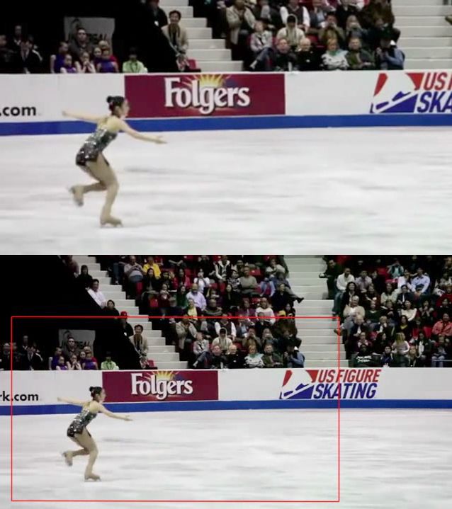
camera path Pt = Ct Bt as described in section 2, and (3)                  400                                            400

stabilizing the video by warping according to Bt .                         300                                            300

    For motion estimation, we track features using pyramidal

                                                                                                                     y
                                                                         y
Lucas-Kanade [12]. However, robustness demands good                        200                                            200

outlier rejection. For dynamic video analysis, global outlier              100                                            100

rejection is insufficient, whereas the short baseline between                 0    40      80       120     160             0      40      80        120   160

adjacent video frames makes fundamental matrix based out-                     (a) w1 = 1, w2 = w3 = 0                       (b) w2 = 1, w1 = w3 = 0
lier rejection unstable. Previous efforts resolve this by un-              500

dertaking 3D reconstruction of the scene via SfM [8], which                                                               400
                                                                           400
is computationally expensive in addition to having stability
                                                                                                                          300
issues of its own.                                                         300

                                                                                                                     y
                                                                          y
    We employ local outlier rejection by discretizing fea-                 200
                                                                                                                          200

tures into a grid of 50×50 pixels, applying RANSAC within                  100                                            100

each grid cell to estimate a translational model, and only re-                0    40      80       120     160             0      40      80        120   160

taining those matches that agree with the estimated model                     (c) w3 = 1, w1 = w2 = 0                  (d) w1 = 10, w2 = 1, w3 = 100
up to a threshold distance (< 2 pixels). We also imple-
                                                                        Figure 8: Optimal path (red) for synthetic camera path (blue)
mented a real-time version of graph-based segmentation [2]
                                                                        shown for various weights of the objective eq. (3).
in order to apply RANSAC to all features within a seg-
mented region (instead of grid cells), which turns out to be
slightly superior. However, we use the grid-based approach              similarities to construct our optimal path. However similar-
for all our results, as it is approximately 40% faster.                 ities (like affine transforms) are unable to model non-linear
                                                                        inter-frame motion or rolling shutter effects, resulting in no-
    Subsequently, we fit several 2D linear motion mod-
                                                                        ticeable residual wobble, which we address next.
els (translation, similarity and affine) to the tracked fea-
tures. While L2 minimization via normal equation with pre-
normalization performs well in most cases, we noticed in-               Residual Motion (Wobble and Rolling Shutter) Sup-
stabilities in case of sudden near-total occlusions. We there-          pression: In order to precisely model inter-frame mo-
fore perform the fit in L1 norm via the LP solver4 , which in-          tion, necessary for complete shake-removal, motion models
creases stability in these cases by automatically performing            with higher DOF than similarities, e.g. homographies, are
feature selection. To our knowledge, this is a novel applica-           needed. However, higher DOF tend of overfit even if out-
tion of L1 minimization for camera motion estimation, and               lier rejection is employed. Consequently, one can achieve
gives surprisingly robust results.                                      good registration for a few frames but their composition
    Once the camera path is computed as set of linear mo-               starts to quickly become unstable, e.g. homographies start
tion models, we fit the optimal camera path according to                to suffer from excessive skew and perspective. We suggest
our L1 optimization framework subject to proximity and                  a robust, hybrid approach, initially using similarities (for
inclusion constraints as described in section 2. A crucial              frame transforms) Ft := St to construct the optimal cam-
question is how to chose the weights w1 − w3 in the objec-              era path, thereby ensuring rigidity over all frames. How-
tive eq. (3)? We explore different weightings for a synthetic           ever, we apply the rigid camera path, as computed, only
path in fig. 8. If only one of the three derivative constraints         for every k = 30 keyframes. For intermediate frames,
is minimized, it is evident that the original path is approxi-
mated by either constant non-continuous paths (fig. 8a), lin-                           Key-Frame
                                                                                                                                                S4
                                                                                                                                                      Key-Frame

ear paths with jerks (fig. 8b), or smooth parabolas but al-                                         S2                    S3                    H4
                                                                         Frame transforms Ft:       H2                    H3
ways non-zero motion (fig. 8c). A more pleasant viewing                  Similarities St &
                                                                         Homographies Ht
experience is conveyed by minimizing all three objectives
                                                                         Optimal
                                                                                                               q1
simultaneously. Though the absolute values of the weights                camera                                      q2
                                                                         path Pt
are not too important, we found eliminating jerks to be most
                                                                                          P1              P2 != P1 S2 T2        P3 = T-14 S-14 P4          P4
important, which is achieved when w3 is chosen to be an or-                                               !   = T-13 S-13 P3
der of magnitude larger than both w1 and w2 .
                                                                        Figure 9: Wobble suppression. The key idea is to decompose the
    The choice of the underlying motion model has a pro-                optimal path Pt into the lower-parametric frame transform St used
found effect on the stabilized video. Using affine transforms           as input and a residual Tt (representing the smooth shift added
instead of similarities has the benefit of two added degrees            by the optimization to satisfy the constraints). St is replaced by
of freedom but suffers from errors in skew which leads to ef-           a higher parametric model Ht to compute the actual warp. For
fects of non-rigidity (as observed by [8]). We therefore use            consistency, the warp is computed forward (red) from previous and
  4 We
                                                                        backward (green) from next key-frame, and the resulting locations
         use the freely available COIN CLP simplex solver.              q1 and q2 are blended linearly.

                                                                  230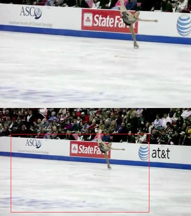
matic pan-and-scan. Simply put, video retargeting falls out
                                                                            as a special case of our saliency based optimization, when
                                                                            the input video is assumed to be stable. In contrast to the
                                                                            work by Liu and Gleicher [7], our camera paths are not con-
                                                                            strained to a single pan, allowing more freedom (e.g. subtle
                                                                            zoom) and adaptation to complex motion patterns.
                                                                                While several measures of saliency exist, we primarily
                                                                            focus on motion-driven saliency. We are motivated by the
                                                                            assumption that viewers direct their attention towards mov-
                                                                            ing foreground objects, a reasonable assumption within lim-
                                                                            itations. Using a fundamental matrix constraint and cluster-
                                                                            ing on KLT feature tracks, we obtain foreground saliency
                                                                            features as shown in fig. 12, which are then used as con-
Figure 10: Reducing rolling shutter by our wobble suppression               straints, as described in section 2.2.
technique. Shown are the result for two frames 1/3 second apart.
Top row: Original frames m (left) and m + 1 (right). Middle                 5. Results
row: Stabilization result without wobble suppression. Bottom
Row: Stabilization with wobble suppression. Notice, how wob-
                                                                            We show some results of video-stabilization using our opti-
ble suppression successfully removes the remaining skew caused              mal camera paths on a YouTube “Fan-Cam” video in fig. 11.
by rolling shutter. (The yellow traffic sign is tilted in reality.)         Our optimization conveys a viewing experience very close
                                                                            to professional footage. In fig. 1, we demonstrate the abil-
we use higher dimensional homographies Ft := Ht to ac-                      ity to include saliency constraints, here derived from a face
count for misalignments. As indicated in fig. 9, we de-                     detector, to frame the dancing girl at the center of result-
compose the difference between two optimal (and rigid)                      ing video without sacrificing smoothness. In the accompa-
adjacent camera transforms, P1−1 P2 , into the known es-                    nying video, the reader will notice occasional blur caused
timated similarity part S2 and a smooth residual motion                     by high motion peaks in the original video. Stabilization
T2 , i.e. P1−1 P2 = S2 T2 (T2 = 0 implies static cam-                       techniques pronounce blur, as the stabilized result does not
era). We then replace the low-dimensional similarity S2                     agree with the perceived (blurred) motion. In the video we
with the higher-dimensional homography H2 , resulting in                    show our implementation of Matsushita et al.’s [10] blur re-
P1−1 P2 := H2 T2 . For each intermediate frame, we con-                     moval technique; however, the blur is too pronounced and
catenate these replacements starting from its previous and                  the technique, suffering from temporal inconsistencies, per-
next keyframes. This effectively results in two sample loca-                forms poorly. However, our framework allows for the intro-
tions q1 , q2 per pixel (indicated with red and green in fig. 9),           duction of motion constraints, i.e. after determining which
with an average error of around 2 − 5 pixels in our experi-                 frames are blurred, we can force the optimal camera path
ments. We use linear blending between these two locations                   to agree with the motion of the blur. This effectively re-
to determine a per-pixel warp for the frame.                                duces the perceived blur while still maintaing smooth (but
                                                                            accelerated) camera motion.
4. Video Retargeting                                                            We demonstrate the ability to reduce rolling shutter in
                                                                            fig. 10; notice how the skew of the house is removed. Us-
Video retargeting aims to change the aspect ratio of a                      ing motion based saliency constraints we can perform video
video while preserving salient and visually prominent re-                   retargeting using a form of automated pan-and-scan in our
gions. Recently, a lot of focus has been on “content-aware”                 framework; see fig. 12 for an example. While we effectively
approaches that either warp frames based on a saliency                      crop the frame, our technique is extremely robust, avoiding
map [14] or remove and duplicate non-salient seams [11, 4],                 spatial and temporal artifacts caused by other approaches.
both in a temporally coherent manner.                                           As dynamics are impossible to judge from images, we
   In section 2.2, we showed how we can direct the crop                     would encourage the reader to watch the accompanying
window to include salient points without having to sacri-                   video. We evaluate our approach on wide variety of videos,
fice smoothness and steadiness of the resulting path. On                    comparing our video stabilization to both current methods
the other hand, if the input video is already stable, i.e. C(t)             of Liu et al. [8, 9]. We also include an example comparing
is smooth, we can explicitly model this property by side-                   the light field approach of Brandon et al. [13]. For video re-
stepping the estimation of each frame transform Ft , and                    targeting, we show more examples and compare to [11, 14].
force it to the identity transform Ft = I, ∀t. This allows                      Our technique is based on per-frame feature tracks only,
us to steer the crop window based on saliency and inclu-                    without the need of costly 3D reconstruction of the scene.
sion constraints alone, achieving video retargeting by auto-                We use robust and iterative estimation of motion models

                                                                      231
Figure 11: Example from YouTube “Fan-Cam” video. Top row: Stabilized result, bottom row: Original with optimal crop window. Our
system is able remove jitter as well as low-frequency bounces. Our L1 optimal camera path conveys a viewing experience that is much
closer to a professional broadcast than a casual video. Please see video.

                                                                          fectively falling back to the shaky video. Further, the use of
                                                                          cropping discards information, something a viewer might
                                                                          dislike. Our computed path is optimal for a given crop win-
                                                                          dow size, which is the only input required for our algorithm.
                                                                          In future work, we wish to address automatic computation
                                                                          of the optimal crop size, as currently we leave this as a
                                                                          choice to the user.

                                                                          Acknowledgements We thank Tucker Hermans for nar-
Figure 12: Example of video retargeting using our optimization
                                                                          rating the video and Kihwan Kim for his selection of fan-
framework. Top row: Original frame (left) and our motion aware
saliency (right). Foreground tracks are indicated by red, the de-
                                                                          cam videos. We are especially grateful to the YouTube Ed-
rived saliency points used in the optimization by black circles.          itor team (Rushabh Doshi, Tom Bridgwater, Gavan Kwan,
Bottom row: Our result (left), Wang et al.’s [14] result (middle)         Alan deLespinasse, John Gregg, Eron Steger, John Skidgel
and Rubinstein et al.’s [11] result (right).                              and Bob Glickstein) for their critical contributions during
                                                                          deployment, including distributed processing for real-time
(from lower to higher dimensional), only using inliers from               previews, front-end UI design, and back-end support.
the previous stage. Our technique is fast; we achieve 20 fps              References
on low-resolution video, while wobble suppression requires                 [1] C. Buehler, M. Bosse, and L. McMillan. Non-metric image-based rendering
grid-based warping and adds a little more overhead. Our                        for video stabilization. In IEEE CVPR, 2001. 226
unoptimized motion saliency runs at around 10 fps.                         [2] P. Felzenszwalb and D. Huttenlocher. Efficient graph-based image segmenta-
                                                                               tion. IJCV, 59(2), 2004. 230
                                                                           [3] M. L. Gleicher and F. Liu. Re-cinematography: Improving the camerawork of
                                                                               casual video. ACM Trans. Mult. Comput. Commun. Appl., 2008. 225, 226
6. Conclusion, Limitations, and Future Work                                [4] M. Grundmann, V. Kwatra, M. Han, and I. Essa. Discontinuous seam-carving
                                                                               for video retargeting. IEEE CVPR, 2010. 231
We have proposed a novel solution for video stabiliza-                     [5] M. Irani. Multi-frame correspondence estimation using subspace constraints.
tion and retargeting, based on computing camera paths di-                      Int. J. Comput. Vision, 48:173–194, July 2002. 226
rected by a variety of automatically derived constraints. We               [6] S.-J. Kim, K. Koh, S. Boyd, and D. Gorinevsky. l1 trend filtering. SIAM Review,
                                                                               2009. 226
achieve state-of-the-art results in video stabilization, while             [7] F. Liu and M. Gleicher. Video retargeting: automating pan and scan. In ACM
being computational cheaper and applicable to a wider va-                      MULTIMEDIA, 2006. 231
riety of videos. Our L1 optimization based approach ad-                    [8] F. Liu, M. Gleicher, H. Jin, and A. Agarwala. Content-preserving warps for 3d
                                                                               video stabilization. In ACM SIGGRAPH, 2009. 225, 226, 230, 231
mits multiple simultaneous constraints, allowing stabiliza-                [9] F. Liu, M. Gleicher, J. Wang, H. Jin, and A. Agarwala. Subspace video stabi-
tion and retargeting to be addressed in a unified framework.                   lization. In ACM Transactions on Graphics, volume 30, 2011. 226, 231
A stabilizer based on our algorithm, with real-time pre-                  [10] Y. Matsushita, E. Ofek, W. Ge, X. Tang, and H.-Y. Shum. Full-frame video
                                                                               stabilization with motion inpainting. IEEE Trans. Pattern Anal. Mach. Intell.,
views, is freely available at youtube.com/editor.                              28, July 2006. 225, 231
    Our technique may not be able to stabilize all videos,                [11] M. Rubinstein, A. Shamir, and S. Avidan. Improved seam carving for video
                                                                               retargeting. In ACM SIGGRAPH, 2008. 231, 232
e.g. low feature count, excessive blur during extremely fast
                                                                          [12] J. Shi and C. Tomasi. Good features to track. In IEEE CVPR, 1994. 230
motions, or lack of rigid objects in the scene might make                 [13] B. M. Smith, L. Zhang, H. Jin, and A. Agarwala. Light field video stabilization.
camera path estimation unreliable. Employing heuristics to                     In ICCV, 2009. 226, 231
detect these unreliable segments, we reset the correspond-                [14] Y.-S. Wang, H. Fu, O. Sorkine, T.-Y. Lee, and H.-P. Seidel. Motion-aware
                                                                               temporal coherence for video resizing. ACM SIGGRAPH ASIA, 2009. 231, 232
ing linear motion models Ft to the identity transform, ef-

                                                                    232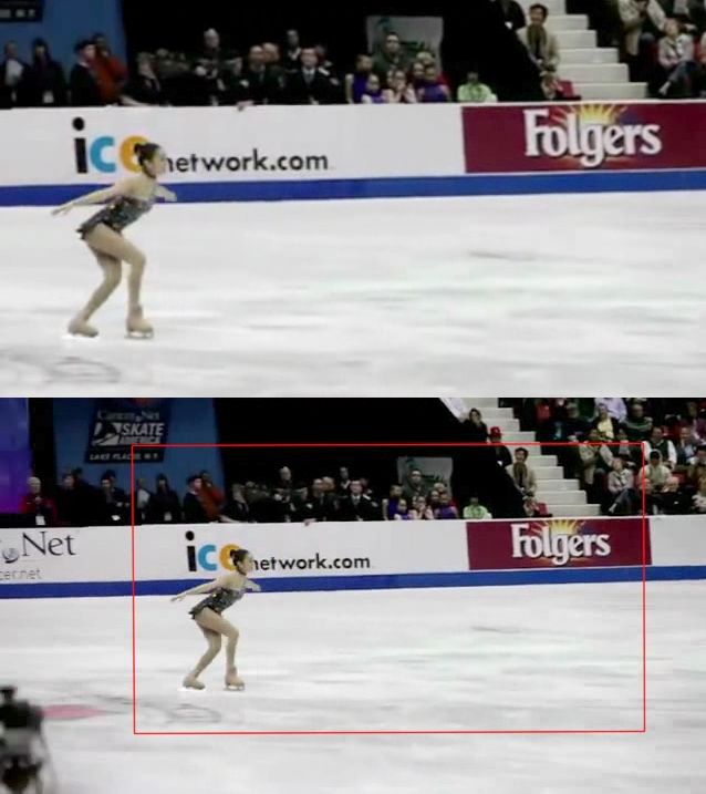
You can also read