Better that X guilty persons escape than that one innocent suffer
←
→
Page content transcription
If your browser does not render page correctly, please read the page content below
Better that X guilty persons escape
            than that one innocent suffer
               Matteo Rizzolli∗and Margherita Saraceno†
                                   June 16, 2009

                                     Abstract
          The principle that it is better to let some guilty individuals be
      set free than to mistakenly convict an innocent person is generally
      shared by legal scholars, judges and lawmakers of modern societies.
      The paper shows why this common tract of criminal procedure is also
      efficient. We extend the standard Polinsky & Shavell (2007) model of
      deterrence to account for the commonly found bias against wrongful
      convictions (Type I) errors and in particular we show that while it
      is always efficient to minimize the number of Type I errors, a more
      than minimal amount of wrongful acquittals (Type II errors) may be
      optimal.

         Keywords: Type I errors, Type II errors, evidence, optimal under-
      deterrence, Blackstone.
         JEL classification: K14, K41, K42.

∗
    University of Milano-Bicocca
†
    University of Milano-Bicocca

                                         1
1 Introduction
A cornerstone of criminal procedures in modern democracies (and also in
advanced societies of the past) is the robust protection granted to defendants
through several procedural safeguards. Most of these mechanisms protect
the innocent from mistaken convictions at the cost of allowing some guilty
defendants to be set free. As Blackstone puts it: it is better that ten guilty
persons escape, than that one innocent suffer (1766). More generally, it can
be argued that it is better that “X > 1” guilty persons escape punishment
than that one innocent person suffers. We will refer to the ratio between
guilty persons wrongfully acquitted and innocent persons unjustly convicted
as the Blackstone error ratio.
Incontrovertible as it seems, this characteristic of criminal procedure
meets with little analysis from law & economics scholars. Standard mod-
els of deterrence consider both types of errors (convictions of the innocent
and acquittals of the guilty) and show that they are both detrimental to
deterrence (See Png, 1986; Polinsky and Shavell, 2007). They come to this
conclusion observing that acquittals of guilty individuals dilute deterrence
because they lower the probability of conviction, while convictions of the
innocent lower the relative benefits of staying honest. According to these
models, and under a number of other assumptions1 , the authority should
treat both types of errors as equal evils to deterrence. But if they are both
equally bad in terms of deterrence, why should we care about minimizing
convictions of the innocent even at the cost of allowing many acquittals of
guilty individuals? In other words: is the Blackstone error ratio inefficient
or do our models miss something from the picture? In the rest of this paper
we will offer an extension of the standard model of optimal deterrence that
reconciles the efficiency goals of the judicial system with the Blackstone error
ratio. The paper is arranged as following: in the first part we introduce the
Blackstone error ratio, and we give a brief overview of the literature. Then
we introduce our model and show how the standard model of deterrence, if
duly articulated to account for the social welfare implications of both Type
I and Type II errors, explains the bias against Type I errors. We then derive
some policy implications and conclude.
1
such as the fact that deterrence is the goal of criminal law, that individuals are rational
expected utility maximizers and are neutral to risk.
22 Judicial errors in the literature
The trade-off between the two types of error has been known and discussed
by lawyers and philosophers for a long time. Courts make recurrent men-
tion of it and this seems to point at the case of a conscious and intentional,
albeit not systematized, pursuit of a specific ratio of innocent convicted to
guilty acquitted that is more favorable to the innocent. How much more
favorable? While every court and scholar would agree that it is desirable to
reduce Type I errors, how many more Type II errors are we willing to toler-
ate in order to achieve this goal? Every American student of law learns by
heart Judge Blackstone’s maxim that gives this paper its title. The United
States Supreme Court has recalled Blackstone’s principle although it has
never committed to such a precise number2 . Countless scholars have men-
tioned a precise number for this trade-off; however, as Volokh (1997) has
pointed out, there is a great variety of opinions on what this number should
be. Volokh finds mentions of the type−II
type−I
trade-off that date back to Gene-
sis and historically vary at least between X = 10004 to X = 15 . As seen,
3
Blackstone asserts that the optimal X must be equal to 10. However this is
a severe underestimation if compared to, for instance, Benjamin Franklin’s
figure of X = 1006 and some other wildly inflated numbers mentioned in the
literature7 ; but at the same time it looks pretty generous if compared with
2
The Supreme Court cited Blackstone in “Coffin v. U.S”., 156 U.S. 432 (1895). For
direct mention of the trade-off see for instance “Herny v. United States” 61 U.S. 98 (1959):
“It is better, so the Fourth Amendment teaches, that the guilty sometimes go free than
that citizens be subject to easy arrest”, or the concurrent opinion of Judge Harlan in “In
re Winship” 397 U.S. 358 (1970) where he states: “I view the requirement of proof beyond
a reasonable doubt in a criminal case as bottomed on a fundamental value determination
of our society that it is far worse to convict an innocent man than to let a guilty man go
free”.
3
Judge Blackstone’s quotation in the title is a reference to Genesis 18:23-32.
4
Moses Maimonidies, a Jewish Spanish legal theorist, interpreting the commandments
of Exodus. Cited in Volokh (1997).
5
Justinian’s Digest. 48.19.5pr. (Ulpianus 7 de off. procons.) sed nec de suspicionibus
debere aliquem damnari divus traianus adsidio severo rescripsit: satius enim esse impuni-
tum relinqui facinus nocentis quam innocentem damnari. Also cited in Volokh (1997).
6
“it is better [one hundred] guilty Persons should escape than that one innocent Person
should suffer”. Letter from Benjamin Franklin to Benjamin Vaughan (Mar. 14, 1785), in
Franklin and Smyth (1970) cited in Volokh (1997).
7
See also Reiman and van den Haag (1990).
3– for instance – Hale’s X = 58 or Ayatollah Hossein Ali Montazeri’s X = 19 .
Irony aside, the Blackstone error ratio in its extremely variegated declina-
tions expresses the principle that, for a number of reasons, it is better that
the criminal procedure produces more mistakes against society (acquittal of
the guilty) than against individuals (conviction of the innocent), under the
assumption that the total number of mistakes, given a certain level of foren-
sic technology, is irreducible below a certain threshold. Better that some
criminals be set free than that any innocent person be jailed, or, to use the
law & economics jargon of Judge Posner (1999), the costs of convicting the
innocent far exceed the benefits of convicting one more guilty individual. To
conclude, there appears to be an enduring preference, even across different
legal systems, for allowing concern over the possible wrongful conviction of
an innocent individual to prevail over the desire for the apprehension of a
guilty one.
Has law & economics explained this characteristic of criminal procedure?
There are a number of papers that postulate the Posnerian assertion that
Type I errors are far worse than Type II errors, and simply weight the two
errors differently in their functions of social costs (See Miceli, 1991; Lando,
2009). Harris (1970) first extends Becker’s (1968) model to include the social
costs of Type I errors. Ehrlich (1982) adds an independent term that mea-
sures the social costs of miscarriage of justice to his function of the social
costs of crime that society needs to minimize. In any case, these models do
not explain the Blackstone bias but simply assume it and express the bias by
weighting the two errors differently. As we will see, our model explains this
different weight from within the model. Indeed one could still feel the need
to weight Type I errors more than Type II errors, for other reasons which we
do not address in this paper, and this would reinforce our main conclusions.
Some recent literature tries to endogenize the Blackstone error ratio. Hyl-
ton and Khanna (2007) develop a public-choice account of the pro-defendant
mechanisms in criminal procedure that affect the Blackstone error ratio as
a set of safeguards against the prosecutor’s potential misconduct. In their
view the Blackstone error ratio is the result of a second-best equilibrium
achieved within the constraint of an irreducible inclination of prosecutors
to over-convict defendants (for various public-choice reasons). Persson and
8
Hale and Emlyn (1736) cited in May (1875).
9
“In Islam, it is better if a guilty person escapes justice than that an innocent man
receives punishment.” International news, Reuters, November 23, 1985. Cited in Volokh
(1997).
4Siven (2007) formulate a general equilibrium model of crime deterrence where
the Blackstone error ratio for capital punishment emerges endogenously as
a result of a median voter mechanism applied to courts. Both models de-
part from the standard model of deterrence. We derive justifications for the
Blackstone error ratio straight from the standard model of public enforce-
ment of law as set out definitively by Polinsky and Shavell (2007). We also
extend their framework to model the behavior of the adjudicative authority
and we show how the comonly observed paucity in producing Type I errors
(even at the cost of producing many Type II errors) is perfectly explained in
terms of optimal deterrence.
3 The Model
All criminal procedures in modern democracies presume the defendant’s in-
nocence until proven guilty. To put it in statistical terms, the innocence of
the defendant is the null hypothesis which the courts are presented with and
which prosecutors try to confute. Courts, hearing the opposing arguments
of the parties, decide on the basis of the evidence presented. We set the
null hypothesis on the option that the accused is innocent10 . An incorrect
rejection of the null hypothesis corresponds to the conviction of an innocent
person and implies a Type I error whereas an incorrect acceptance of the
null amounts to the acquittal of a guilty person and is described as a Type
II error11 . The sum of the two errors is considered a rough measure of the
accuracy of adjudication (Kaplow, 1994).
Let e ∈ [0, ∞] be the prosecutor’s differential ability to convince the court
of the defendant’s guilt. The capacity of the prosecutor to prove guilt varies
with each accused as individuals have different abilities to confute the allega-
tions of guilt before the court. These differential abilities depend upon, inter
alia, i) the capacity to afford good lawyers (which is independent of either
actual innocence or guilt) and the ease with which exculpatory evidence can
10
Here we set the null hypothesis on the option that the defendant is innocent. For
various reasons it is more common to find in the literature the null hypothesis set on the
option that the defendant is guilty. See for instance Polinsky and Shavell (2000); Persson
and Siven (2007). Hence they obtain definitions of Type I and Type II errors that mirror
ours.
11
On the use of statistics in evidence see also Yilankaya (2002); Posner (1999); McCauliff
(1982); Daughety and Reinganum (2000); Froeb and Kobayashi (2001). For a critical
perspective see Allen and Pardo (2007).
5be produced (which in contrast is dependent upon innocence/guilt). It is rea-
sonable to assume that, on average, the prosecutor’s ability to prove the guilt
of innocent persons is low, whereas it is relatively high in respect of guilty
individuals. Thus, let us define I(e) as the positive, continuous and differen-
tiable cumulative function of e for innocent individuals. Furthermore, let us
define G(e) as the positive, continuous and differentiable cumulative function
of e for guilty individuals.12 G(e) has first-order stochastic dominance over
I(e).
In order to obtain a conviction, a certain threshold of e must be overcome.
Suppose the court rejects the null hypothesis when the prosecutor reaches
an e > ẽ . The probability of convicting an innocent person is thus 1 − I(ẽ).
The probability of convicting a criminal is 1 − G(ẽ). This case is represented
in figure 1.
In figure 1 above, we note that when we increase the burden of evidence
(ẽ → ẽ" ) necessary to obtain a conviction, we reduce the probability of con-
viction both for guilty and for innocent individuals as 1 − I(ẽ" ) < 1 − I(ẽ)
and 1−G(ẽ" ) < 1−G(ẽ). Note that the probability of convicting an innocent
individual 1 − I(ẽ) is also the probability of Type I error, and the probability
of acquitting a guilty individual G(ẽ) represents the probability of Type II
error. Thus when the burden of evidence increases, the probability of Type
II error also increases while the probability of Type I error decreases.
Other changes may happen when better forensic technology is introduced
that allows the prosecutor to collect better evidence of guilt and thus helps
the court to better distinguish guilty individuals from innocent ones. For
a given standard of evidence (ẽ) required by the procedure, better forensic
technology usually improves the ability of the prosecutor to produce incrim-
inating evidence for the guilty and reduces it for the innocent. This implies
that the distributions of the differential abilities are less dispersed and more
distinguishable (See figure 1). Note that improved forensic technology on
average reduces both the probability of Type I error as 1 − I " (ẽ) < 1 − I(ẽ)
and the probability of Type II error as G" (ẽ) < G(ẽ).
We distinguish between a long-term horizon where changes in the stan-
dard of evidence and in forensic technology may happen and the short-term
horizon where these are fixed. Arguably a modern lawmaker should aspire to
12
An alternative way of thinking of it is to simply assume e to be the incriminating
proofs for the defendant. We can assume that the prosecutor can gain more proofs against
a guilty defendant than against an innocent one. G(e) and I(e) are the cumulative function
of proofs against the guilty and the innocent respectively.
6Figure 1: Probability distributions of the authority’s differential ability to
prove guiltiness, for guilty and innocent persons.
7obtain a legal framework that produces zero errors of any type. However, as
Harris (1970) shows, in the long term social preferences may favor different
regimes and the political process may build on one extreme some “law and
order” or “zero tolerance” type of equilibrium compatible with a high num-
ber of Type I errors or on the other extreme a very radical approach to civil
liberties that imposes a very high number of Type II errors. Depending on
these long-term trends, a society sets (by statute or case law) the standard of
evidence necessary for a court to convict. The court thus in the short term
faces an exogenously determined ẽ.
Of course in the long term forensic technology also improves. Knowledge
and technical discoveries can be thought of as irreversible so the distance
between the two distribution necessarily widens in time. We can imagine
that in the short term courts may voluntarily surrender the use of more
accurate technology in order to contain costs13 .
In the short term, which is our main horizon of analysis, the set of rules,
the standard of proof and the forensic technologies are given. These techno-
logical and legal constraints imply a lower bound on errors: in the short term
the court system generates at its best a given probability of Type I error equal
to ε1 min ∈ [0, 1), and a minimum probability of Type II error ε2 min ∈ [0, 1).
Of course courts may produce higher error levels because courts still retain
a certain discretion14 . Note that (1 − ε1 min ) > ε2 min , because of the assump-
tion of first-order stochastic dominance. Let us define the errors’ relation –
G(.)
our Blackstone’s error ratio – as X = TType II
ype I
= (1−I(.)) . In our horizon, the
! "
G(.)
Blackstone’s error ratio X = (1−I(.)) falls within ε2 min , ε1 min . Let us define
1
X# as ε2 min and note that it falls within the interval.
ε1 min
3.1 Individual choice to commit crime
Let us define w as the individual differential gain from crime; w is a random
variable with a certain probability distribution z and a certain cumulative
distribution Z.
Let q be the probability of detection, 0 < q ≤ 1, that is to say the
probability that the police accuse an individual (either innocent or guilty)
13
See further in the text; in particular the discussion of Proposition 3.
14
For instance prosecutors and judges may be particularly unskilled, ignorant or ideo-
logically biased. Or they might wilfully fail to make use of all the legal tools or accurate
forensic technologies at their disposal.
8of a crime. In this model, q is exogenous as it simply depends on police
efficiency or on nature15 . Once the police detect an individual they bring
him to court where he goes through the procedure that establishes whether
he is to be convicted and sentenced.
Note that probability of detection q and the probabilities of Type I and
Type II errors are independent. In fact the probabilities of error depend only
on innocence/guilt and on the procedural, institutional and technological
setting.
cp is the private cost of the sentence. This could be either a monetary
loss in case of a fine or the disutility suffered because of imprisonment.
Individuals, who are assumed to be rational and risk-neutral, choose to
stay innocent or to commit a crime by comparing the expected utility of
staying innocent −q (1 − I(ẽ)) cp and the expected utility of committing the
crime w − q(1 − G(ẽ))cp . Thus, the individual condition for committing a
crime is:
w − q(1 − G(ẽ))cp > −q (1 − I(ẽ)) cp (1)
and therefore, in order to commit a crime the individual gain from crime
must be such that w > w̃ where
# = qcp [I(ẽ) − G(ẽ)]
w (2)
We can identify a “deterrence effect” à la Becker (1968). Note that w #
increases with both the probability of detection and the private costs of
punishment (↑ q, cp ⇒↑ w) # . We can also observe an “underdeterrence effect”
of judicial acquittals of guilty individuals as w
# decreases when the probability
of mistaken acquittal increases (↑ G(ẽ) ⇒ ↓ w). # Similarly we can identify
a “compliance effect” of Type I errors (↑ I(ẽ) ⇒ ↑ w) # as w# increases when
correct convictions increase (and thus Type I errors decrease).
Finally, we can also identify a “screening effect”. Let us define (I(ẽ) −
G(ẽ)) = ∆(.) as the difference between the probabilities of being acquitted
respectively when innocent and guilty. ∆(.) represents the ability of the
court to distinguish innocent from guilty individuals: the better the court can
distinguish between innocent people and criminals, the higher the advantages
of staying honest (↑ ∆(.) ⇒↑ w). # Note that equation 2 can also be rewritten
as: I(ẽ) − G(ẽ)) ≥ qcp . From an individual perspective, the left term of
w
15
On different detection technologies see Mookherjee and Png (1992).
9the inequality represents the minimum “distance” between the probability
of being acquitted when innocent and the probability of being acquitted
when guilty that induces an individual to stay honest. Thus a certain ability
to screen between innocent and guilty is necessary to guarantee that some
people stay honest. This distance increases with w and decreases with the
expected private cost of conviction (qcp ).
3.2 Social perspective
Criminal activities and the enforcement system imply three costs. First, the
conviction of a defendant implies a private cost (cp ) for the individual (the
disutility suffered because of the conviction) and also a social cost (cs ). The
social costs of the conviction are the costs of imprisonment (Polinsky and
Shavell, 1984) and more generically the enforcement costs of both monetary
and non-monetary penalties (Polinsky and Shavell, 1992). Moreover, there
is h which is the harm caused to society caused by the crime. For simplicity,
we assume that w is a transfer from the victim to the criminal that cancels
out in the social welfare function. However, this forced transfer may produce
h which is the socially relevant externality caused by the crime.
The population is normalized to 1. We assume the social planner to be
risk-neutral and to have the goal of maximizing social welfare. Thus, for a
given set of rules (mainly, the standard of evidence needed ẽ) the problem of
the authority lies in defining the optimal level of judicial errors in order to
minimize the expected total costs from crime (T C).
T C = [1 − Z(w)]h
# + [1 − Z(w)]q
# (1 − G(.)) [cs + cp ]
$ %& ' $ %& '
A B
# (1 − I(.)) [cs + cp ] (3)
+ Z(w)q
$ %& '
C
Term A of equation (3) represents the expected social harm from crime;
Term B represents expected total (private and social) costs of convicting
criminals; and Term C represents expected total costs of convicting innocent
people. By looking at equation (3) some preliminary considerations can be
made. Consider Term A. We already know from Png (1986) that a surge in
both errors dilutes deterrence and increases the probability that individuals
10become criminals16 [1 − Z(w)].
# Thus in Term A, both errors equally increase
the social costs of crime [h]. However, our equation (3) shows that there
are differences in the way the two errors affect deterrence. Note that Type
II errors [G(.)] ambiguously affect the expected social costs of convicting
criminals: on the one hand they increase the number of criminals [1 − Z(w)] #
but on the other hand (by definition) they reduce the probability of convicting
any criminal (Term B). Finally, Type II errors reduce the number of innocent
people and thus decrease the social cost of convicting an innocent person
(Term C). Now let us focus on Type I errors [1 − I(.)]. We have already seen
in Term A that Type I errors dilute deterrence and thus increase the social
harm of crime [h]. Term B shows that Type I errors increase the number
of criminals and thus unambiguously increase the social costs of convicting
criminals. However, we see in Term C how Type I errors ambiguously affect
the expected social costs of convicting innocent people: on one hand they
increase the probability of convicting an innocent person (by definition) but
on the other hand they decrease the pool of innocent people Z(w). # Thus,
Type I and Type II errors determine multiple and complex effects on the
three addenda of the social function. The table summarizes these effects.
Error effects on the addenda: A B C
Type I (1− I(ẽ)) ↑ ↑ ↑↓
Type II (G(ẽ)) ↑ ↑↓ ↓
Table 1: The effects of the two errors on the addenda of equation 3
We can conclude that the net effects of both judicial errors on the social
cost of crime appear ambiguous. In order to disentangle these effects we
proceed by specifying the distribution of w and by deriving equation (3).
4 The optimal Blackstone ratio with a Pareto
distribution
For a given set of rules (ẽ, forensic technology), the short-term goal of the
social planner is to identify the optimal level of Type I and Type II errors in
16
See section (A.1 and A.2) for the derivation of the result when applying the Pareto
distribution.
11order to minimize the social costs of crime. Thus
min T C (4)
I(.);G(.)
s.t. w# = qcp ∆(.)
s.t.∆(.) > 0
In order to derive this result in the following part of the paper we as-
sume that w is distributed with a Pareto distribution z(w; k, wmin ), where,
as usual, k > 017 , wmin > 0 and the distribution is supported in the interval
[wmin , ∞]. We use the Pareto distribution because it is both positively de-
scriptive and mathematically tractable. As for the first reason, we know how
well the Pareto distribution fits the usually observed distribution of wealth
and income18 (Pareto, 1896; Levy and Solomon, 1997). This is because the
long right tail describes inequality, that is to say the possibility of a few ex-
tremely large outcomes. The Pareto distribution also fits well with the gains
from crime we try to model in this paper. In fact the Pareto distribution
describes well the possibility of having quite a large number of individuals
who can extract minor gains from petty crime and a small number of crim-
inals that can get extremely large outcomes from serious crime and so on19 .
Besides, the Pareto distribution is also mathematically convenient. How-
ever this assumption is without loss of generality: by assuming a generic,
well-behaved distribution function our results do not change, but analysis
becomes intractable. Note that z is independent of the two probability dis-
tributions of the prosecutor’s differential abilities of convincing the court of
17
k is the Pareto index (since a proportion must be between 0 and 1, inclusive, the
index must be positive). The larger the Pareto index, the smaller the proportion of very
high-income people.
18
The Pareto distribution also describes a range of situations including insurance (where
it is used to model claims where the minimum claim is also the modal value, but where
there is no set maximum). Other social, scientific, geophysical and actuarial phenomena
are sometimes seen as Pareto-distributed. For instance the sizes of human settlements -
few cities, many villages; the standardized price returns on individual stocks; the severity
of large casualty losses for certain lines of business such as general liability and so on.
19
Consider a homicide: some criminals could extract very high gains because for instance
the homicide allows them to control a gang or extract a high rent while if the same homicide
is carried out by a drug addict suffering withdrawal symptoms it could lead to few and
very short-term gains. Consider also the peddling of a given amount of cocaine. A well
organized criminal may extract high gains from it while it could easily land a clumsy crook
in trouble.
12the defendant’s guilt. Given a Pareto distribution of the gains from crime w,
the probability that an individual commits the crime is equal to:
( )−k
#
w
# = 1 − Z(w)
Pr(w > w) # = (5)
wmin
Lemma 1. I ∗ (.) = 1 − ε1 min . In order to minimize the social costs of
crime, no innocent person should be convicted because the optimal probability
of Type I error is the smallest possible one.
As shown in the Appendix (A.3), ∂(1−I(.))∂T C
> 0 =⇒ (1 − I(.))∗ = ε1 min .
The optimal level of Type I error is a corner solution in the interval [ε1 min , 1).
The normative implication of this lemma is that courts must convict as few
innocent people as possible given the procedure and forensic technology that
are in place. This result is not trivial given the different effects that the Type
I error has on the different addenda of equation (3).
Lemma 2. G∗ (.) < 1. In order to minimize the social costs of crime,
at least some criminals must be convicted because the optimal probability of
Type II errors is always smaller than 1.
As shown in the Appendix (A.4) the first and second-order conditions
∂2T C
imply ∂G(.)
∂T C
= 0 and ∂G ∗ (.)2 > 0. According to the first and second-order
conditions G (.) = I (.) − ∆∗ (.). Now from Lemma 1 we substitute I ∗ =
∗ ∗
(1 − ε1 min ) and obtain G∗ (.) = (1 − ε1 min ) − ∆∗ (.) which is always lower
than 1. This lemma simply states that optimal deterrence needs at least
some convictions. This implies that there must be an upper bound in our
Blackstone error ratio X and thus some of the severely inflated numbers we
have seen in Section 2 are likely not to lead to optimal deterrence.
Proposition 1. G∗ (.) ≥ e2min . If the costs of conviction are sufficiently
high (relative to the social harm of crime), then some under-deterrence in
the form of Type II errors is efficient.
Even when the legal system is able to produce the ideal value of ε1 min = 0,
G (.) is equal to zero if and only if ∆∗ (.) = 1. Since ∆∗ (.) = 1−k
∗ k h
q[cs +cp ]
(see
13appendix A.4), ∆∗ (.) = 1 if cs +cp = hq 1−k
k
. Therefore if the costs of conviction
are high enough ([cs + cp ] > q 1−k ) the optimal G∗ (.) is an interior solution.
h k
This result has important implications: Whenever punishment is costly,
in order to minimize the social costs of crime at least some criminals must be
acquitted because the optimal probability of Type II errors may be greater
than the smallest possible Type II error.
Corollary 1. Optimal accuracy should be different for serious vis-à-vis
less severe crimes.
Only when the social harm of crime is sufficiently high with respect to the
total costs of conviction, is it then efficient to have Type II errors at their
smallest possible number G∗ (.) = e2min . This implies that no (avoidable)
wrongful acquittal should be allowed for serious crimes (those that produce
high h) while some wrongful acquittals may be efficient for less severe crimes.
Now, focusing on the Type II/Type I error trade-off, note that, for a given
G∗ (.)
set of rules, the optimal Blackstone error ratio X ∗ = (1−I ∗ (.)) .
Proposition 2. X ∗ ≥ X̃. The optimal Blackstone error ratio that minimizes
# = ε2 min .
the social costs of crime may be larger than X ε1 min
Recall that while I ∗ (.) = ε1 min (Lemma 1), G∗ (.) ≥ e2min ( Proposition
1), at least when the costs of convictions are sufficiently high vis-à-vis the
severity of the crime. Therefore the optimal Blackstone error ratio is X ∗ =
G∗ (.)∈[ε2 min ,1)
ε1 min
. Note that Xmin < X̃ ≤ X ∗ < Xmax , where Xmin = ε2 min and
Xmax = ε1 1min .
It is trivial to show that when the costs of conviction are zero, judicial
errors affect only the probability of crime and the optimal Type I and Type
II errors are equal to the lowest values possible (X ∗ #
= X).
(cs =cp =0)
Finally, for every “short term” equilibrium, when the forensic technology
and therefore ε1 min and ε2 min are given, we know that
14*
I ∗ (.) = 1 − ε1 min
k h
∆∗ (.) = 1−k q[cs +cp ]
Proposition 3: ∆∗ (.) depends negatively on the social costs of conviction
and positively on the harm caused by crime and on the Pareto index k.
∆∗ (.) is the optimal “distance” between the probability of being acquitted
when innocent and the probability of being acquitted when guilty. As such it
could be interpreted as the court’s optimal ability to distinguish between in-
nocence and guilt. Note that ∆∗ (.) is non-negative and that this is consistent
with stochastic dominance. Furthermore, its first derivative with respect to
its determinants respectively are
*
∂∆∗ (.) ∂∆∗ (.)
∂h
, ∂k > 0
∂∆∗ (.) ∂∆∗ (.) ∂∆∗ (.)
∂cs
, ∂cp , ∂q5 Conclusions and Policy Implications
The criminal procedure is inherently exposed to the risk of producing Type I
and Type II errors. Some forms of safeguards against the occurrence of Type
I errors (wrongful convictions) are embedded in the procedures of all mod-
ern liberal states, although this inevitably implies that more Type II errors
(wrongful acquittals) are produced. In other words, all modern procedures
are constructed in order to produce a Blackstone error ratio X > 1. With
this paper we show that the standard model of public enforcement of law
(as expounded by Polinsky and Shavell, 2007) can explain this bias and that
even a large Blackstone error ratio is compatible with the standard model
of deterrence. In this paper we focus only on the production of the judi-
cial error at the court level and we take all other important variables of the
Becker framework (such as the magnitude of punishment and the probabil-
ity of detection) as given. We show that while courts should always strive
to minimize Type I errors, they may let some Type II errors happen even
where these could be avoided, if the costs of convictions are relatively high.
In other words, and similarly to Polinsky and Shavell (1992), we show that
some under-deterrence may be optimal20 if the costs of conviction are sig-
nificant relative to the social harm. This could happen when for instance
the prison system is inefficient or whenever petty crimes do not cause great
social harm.
The intuition of the model is quite simple. From basic decision theory,
we know that the two errors are inversely related: for instance, by raising
the standard of proof we obtain more Type II errors and fewer Type I errors.
Thus, suppose we have an error ratio of 1: there is exactly one Type II
error for every Type I error. If we can slightly affect the ratio by adding
and subtracting two arbitrary small quantities, ρ and σ , to the Type II and
Type I probabilities respectively such that TType II+ρ
ype I−σ
, then we achieve two
effects. On one hand, one fewer Type I error increases deterrence (because it
increases the expected returns from staying honest) while one more Type II
error decreases deterrence (by increasing the expected returns from crime).
Thus on balance deterrence should stay constant. On the other hand, one
fewer Type I error with one more Type II error decreases the total costs of
conviction and thus increases social welfare. It is thus efficient to trade one
20
However, while Polinsky and Shavell (1992) focus on the detection probability at the
police level, we focus on the trade-off of errors at the court level.
16error for the other. However, this holds true only for small values of ρ and
σ. In fact, since the trade-off of the errors is not linear, at a certain point
one fewer Type I error will be traded off against too many Type II errors,
causing a drop of deterrence that cannot be compensated any further by the
saved costs of conviction in our social welfare function.
Our paper offers an efficiency-based argument in support of the full array
of pro-defendant features (such as mandatory disclosure, double jeopardy,
the right to silence, the high burden of proof and so on) that characterize
criminal procedure in all modern and democratic countries. As we have
seen, all these pro-defendant features invariably alter the error ratio towards
a Blackstone-like quotient. We explain how the associated costs in terms of
decreased deterrence are compensated by lower conviction costs associated
with more guilty defendants being acquitted.
Our proposition 1 and the following corollary have important policy im-
plications. We show that some under-deterrence is efficient if the costs of
conviction offset the social harm of crime (cp + cs > h) . This result shows
that the findings of Polinsky and Shavell (1984) are robust against the in-
troduction of Type I errors. The corollary brings a more novel result, as it
explains why courts should focus more on serious crime (for which no avoid-
able Type II error should be allowed) while they could let some criminals be
acquitted for petty crimes (those with low h). Another policy implication
that comes from the proposition suggests that, when the costs of conviction
(cp ) are high, the court may allow more Type II errors to happen. This could
represent an alternative tool to the clemency bills used in some countries to
contain public deficits, which have adverse consequences for overall deter-
rence and the perception of the rule of law (see for instance Drago et al.,
2009).
The model highlights the role of forensic technology in improving the
courts’ capacity to distinguish optimally between the innocent and the guilty.
Further work could be done introducing some costs of new technology.
Appendixes
A. First and second-order conditions
We derive the first and second-order conditions of equation 4.
Recall that the gain’s threshold is w # = qcp (I(.) − G(.)) and that the
17+ ,−k
probability of committing a crime given our Pareto distribution is wmin e
w
=
+ ,−k
qcp (I(.)−G(.))
wmin
. In order to see the effects of the two errors on the criminal
population we apply the Pareto distribution as in equation 5 to equation (3).
We then partially derive the equation in respect of the two errors and see
that, as predicted by Png (1986), both errors dilute deterrence.
A.1. The first derivative of the probability of committing a crime with
respect to the complement to one of Type I error - probability of acquitting
an innocent person)
( )−k−1
d qcp #
w
= −k 0 (7)
dG(.) wmin wmin
.
The social function is
( )−k ( )−k
#
w #
w
TC = h+ q (1 − G(.)) [cs + cp ]
wmin wmin
- ( )−k .
w#
+ 1− q (1 − I(.)) [cs + cp ]
wmin
A.3 We derive the first-order conditions: we calculate the first derivative
of T C with respect to the sound convictions (the complement to one of the
probability of Type I error):
( )−k−1
∂T C qcp #
w
= −k [h + q (1 − G(.)) [cs + cp ]]
∂I(.) wmin wmin
( )−k−1 - ( )−k .
qcp #
w w#
+k q (1 − I(.)) [cs + cp ] − 1− q [cs + cp ] =
wmin wmin wmin
18( )−k−1
qcp #
w
= −k [h + q [cs + cp ] (I(.) − G(.))]
wmin wmin
- ( )−k .
w#
− 1− q [cs + cp ] < 0
wmin
=⇒ ∂
∂(1−I(.))
> 0 =⇒ (1 − I(.))∗ = ε1 min
A.4 The first derivative of TC with respect to the probability of Type II
error:
( )−k−1
∂T C qcp #
w
= +k [H + q (1 − G(.)) [cs + cp ]]
∂G(.) wmin wmin
( )−k
#
w
− q [cs + cp ] =
wmin
( )−k−1
qcp #
w
= +k [h + q [cs + cp ] (I(.) − G(.))]
wmin wmin
( )−k
#
w
− q [cs + cp ] ≶ 0
wmin
( )−k−1
qcp #
w
= +k [h + q [cs + cp ] (I(.) − G(.))]
wmin wmin
( )−k
#
w !
− q [cs + cp ] = 0
wmin
h
/ k
0
(I(.) − G(.)) = q[cs +cp ] 1−k
k h
∆∗ (.) = 1−k q[cs +cp ]
≥0
G∗ (.) = I ∗ (.) − ∆∗ (.)
19G∗ (.) = (1 − ε1 min ) − ∆∗ (.) < 1
We also need the second-order condition: with respect to the probability
of Type II error:
( )−k−2
∂2T C qcp qcp #
w
2
= (k + 1) k [h + q [cs + cp ] (I(.) − G(.))]
∂G(.) wmin wmin wmin
( )−k−1
qcp #
w
− 2k q [cs + cp ] > 0
wmin wmin
(k + 1) k wqcmin
p qcp
e
w
[h + q [cs + cp ] (I(.) − G(.))] > 2k wqcmin
p
q [cs + cp ]
! "
2
h > q [cs + cp ] (I(.) − G(.)) (k+1)
−1
1−k
h > q [cs + cp ] (I(.) − G(.)) (k+1)
k h
(I(.) − G(.))∗ = ∆∗ (.) = 1−k q[cs +cp ]
k h 1−k
h > q [cs + cp ] 1−k q[cs +cp ] (k+1)
h> k
(k+1)
h h (k + 1) > kh always true.
The second-order condition always holds in (G∗ , I).
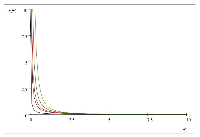
B. The Pareto Distribution
The figures below show the probability density function and the cu mula-
tive distribution function of a Pareto distribution with different shapes and
location wmin = 1
k
k∗wmin
z(w) = k+1
20/w 0k
Z(w) = 1 − min
w
Changes in k (larger than 1) or in wmin do not affect our analysis. Func-
tions are plotted for k = 0.1; 0.3; 0.5; 0.7; 1 (from left to right in the first
figure, from bottom up here above).
21References
Allen, R. J. and M. S. Pardo, “The Problematic Value of Mathematical
Models of Evidence,” Journal of Legal Studies, 2007, 36.
Becker, Gary, “Crime and Punishment: An Economic Approach,” Journal
of Political Economy, 1968, 76, 169–217.
Blackstone, Willian, Commentaries on the laws of England., Vol. 4, Ox-
ford: Clarendon Pr, 1766.
Daughety, A. F. and J. F. Reinganum, “On the economics of trials:
adversarial process, evidence, and equilibrium bias,” Journal of Law, Eco-
nomics, and Organization, 2000, 16 (I2).
Drago, F., R. Galbiati, and P. Vertova, “The deterrent effects of prison:
evidence from a natural experiment,” Journal of Political Economy, 2009,
117 (2), 257–280.
Ehrlich, Isaac, “The Optimum Enforcement of Laws and the Concept of
Justice: A Positive Analysis,” International Review of Law and Economics,
1982, 2, 3–27.
Franklin, Benjamin and Albert Henry Smyth, The writings of Ben-
jamin Franklin, New York,: Haskell House, 1970.
Froeb, L. M. and B. H. Kobayashi, “Evidence Production in Adversarial
vs. Inquisitorial Regimes,” Economics Letters, 2001, 70 (2), 267–272.
Hale, Matthew and Sollom Emlyn, Historia placitorum coronæ. The
history of the pleas of the crown, [London]: In the Savoy, Printed by E.
and R. Nutt, 1736.
Harris, J.R., “On the Economics of Law and Order,” Journal of Political
Economy, 1970, 78 (1), 165.
Hylton, Keith N. and Vikramaditya S. Khanna, “A Public Choice
Theory of Criminal Procedure,” Supreme Court Economic Review, 2007,
15, 61–118.
Kaplow, Louis, “The Value of Accuracy in Adjudication: An Economic
Analysis,” Journal of Legal Studies, 1994, 23 (1), 307–401.
22Lando, Henrik, “Prevention of Crime and the Optimal Standard of Proof
in Criminal Law,” Review of Law and Economics, 2009, 5 (1), 33–52.
Levy, M. and S. Solomon, “New evidence for the power-law distribution
of wealth,” Physica A, 1997, 242 (1-2), 90–94.
May, Wilder, “Some Rules of Evidence: Reasonable Doubt in Civil and
Criminal Cases,” American Law Review, 1875, 10, 642–672.
McCauliff, Catherine M.A, “Burdens of proof, degrees of belief, quanta
of evidence, or Constitutional guarantees?,” Vanderbilt Law Review, 1982,
35, 1293.
Miceli, Thomas J., “Optimal criminal procedure: Fairness and deterrence,”
International Review of Law and Economics, 1991, 11 (1), 3–10.
Mookherjee, D and Ivan P. L. Png, “Monitoring vis-a-vis Investigation
in Enforcement of Law,” The American Economic Review, 1992, 82 (3),
556–565.
Pareto, Vilfredo, Cours d’economie politique, Vol. 2 v, F. Rouge, Lusanne,
1896.
Persson, M. and C.H. Siven, “The Becker Paradox And Type I Ver-
sus Type Ii Errors In The Economics Of Crime,” International Economic
Review, 2007, 48 (1), 211–233.
Png, Ivan P. L., “Optimal Subsidies and Damages in the Presence of Ju-
dicial Error,” International Review of Law and Economics, 1986, 6 (1),
101–05.
Polinsky, A. Mitchell and Steven Shavell, “The optimal use of fines and
imprisonment,” Journal of Public Economics, 1984, 24 (1), 89–99.
and , “The Economic Theory of Public Enforcement of Law,” Journal
of Economic Literature, 2000, 38 (1), 45–76.
and , “The Theory of Public Enforcement of Law,” in A. Mitchell Polin-
sky and Steven Shavell, eds., Handbook of Law and economics, Amsterdam:
Elsevier, 2007.
23Polinsky, A.M. and S. Shavell, “Enforcement costs and the optimal mag-
nitude and probability of fines,” Journal of Law and Economics, 1992,
pp. 133–148.
Posner, Richard A., “An Economic Approach to the Law of Evidence,”
Stanford Law Review, 1999, 51 (6), 1477–1546.
Reiman, Jeffrey and Ernest van den Haag, “On the Common Saying
That It Is Better That Ten Guilty Persons Escape Than That One In-
nocent Suffer: Pro and Con,” Social Philosophi and Policy. Issue Crime,
Culpability, and Remedy, 1990, 7 (2), 226.
Volokh, Alexander, “n Guilty Men,” University of Pennsylvania Law Re-
view, 1997, 146 (1), 173–216.
Yilankaya, Okan, “A Model of Evidence Production and Optimal Standard
of Proof and Penalty in Criminal Trials,” Canadian Journal of Economics,
2002, 35 (2), 385–409.
24You can also read