Autonomous Orbit Determination for a Hybrid Constellation
←
→
Page content transcription
If your browser does not render page correctly, please read the page content below
Hindawi
International Journal of Aerospace Engineering
Volume 2018, Article ID 4843061, 13 pages
https://doi.org/10.1155/2018/4843061

Research Article
Autonomous Orbit Determination for a Hybrid Constellation

          Muzi Li ,1 Bo Xu ,2 and Jun Sun3
          1
            School of Astronomy and Space Science, Nanjing University, Nanjing 210023, China
          2
            School of Aeronautics and Astronautics, Sun Yat-Sen University, Guangzhou 510006, China
          3
            Shanghai Aerospace Control Technology Institute, Shanghai 201199, China

          Correspondence should be addressed to Bo Xu; xubo@nju.edu.cn

          Received 4 March 2018; Revised 6 August 2018; Accepted 13 August 2018; Published 26 September 2018

          Academic Editor: Jose Carlos Páscoa

          Copyright © 2018 Muzi Li et al. This is an open access article distributed under the Creative Commons Attribution License, which
          permits unrestricted use, distribution, and reproduction in any medium, provided the original work is properly cited.

          A new orbit determination scheme targeting communication and remote sensing satellites in a hybrid constellation is investigated
          in this paper. We first design one such hybrid constellation with a two-layer configuration (LEO/MEO) by optimizing coverage and
          revisit cycle. The main idea of the scheme is to use a combination of imagery, altimeter data, and inter-satellite range data as
          measurements and determine orbits of the satellites in the hybrid constellation with the help of the extended Kalman filter
          (EKF). The performance of the new scheme is analyzed with Monte Carlo simulations. We first focus on an individual remote
          sensing satellite and compared the performance of orbit determination using only imagery with its counterpart using both
          imagery and altimeter measurements. Results show that the performance improves when imagery is used with altimeter data
          pointing to geometer calibration sites but declines when used with ocean altimeter data. We then expand the investigation to the
          whole constellation. When inter-satellite range data is added, orbits of all the satellites in the hybrid constellation can be
          autonomously determined. We find that the combination of inter-satellite range data with remote sensing observations lead to a
          further improvement in orbit determination precision for LEO satellites. Our results also show that the performance of the
          scheme would be affected when remote sensing observations on certain satellites are absent.

1. Introduction                                                        proposed. Some of these works focus on autonomous orbit
                                                                       determination based on either optical imagery or altimeter
A hybrid constellation refers to a group of satellites at differ-       data or inter-satellite range data. White et al. [6] used line-
ent orbital regimes working in concert. A widely known                 of-sight (LOS) measurements of stars and landmarks to esti-
example is the BEIDOU navigation satellite constellation of            mate the attitude and orbit of satellites. Straub and Christian
China. The hybrid constellation concept commonly appears               [7] used observations of coastlines on the Earth’s surface as
in studies on navigation constellation design and optimiza-            inputs to autonomously determine the orbits of earth-
tion [1, 2]. It has also been introduced to the fields of satellite     observing satellites with different orbit inclinations and alti-
communication and remote sensing [3, 4], and Fahnestock                tudes. Li, Xu and Zhang [8] proposed a scheme using images
and Erwin [5] presented a kind of hybrid constellation to              of ground objects and analyzed the influence of image resolu-
meet space situation awareness requirements. However, few              tion, pointing accuracy and lighting constraints on the orbit
research tries to design a hybrid constellation as a multifunc-        determination performance. Following that study, Li and
tion constellation.                                                    Xu [9] presented an orbit and attitude determination
    At present, orbit determination for satellites depends             (OAD) scheme using images of regular-shaped ground land-
heavily on the earth stations and navigation constellations            marks to overcome the disadvantages using ground point
(for example, GPS constellation). In order to reduce mainte-           features. As another high-precision measurement, the altim-
nance cost of these systems and enhance survivability of               eter can provide highly accurate altitude information which
satellites in cases of emergencies, autonomous orbit determi-          helps to effectively improve the orbit determination accuracy.
nation methods which depend on instruments on board were               Born et al. [10] determined the orbit of the N-ROSS satellite
2                                                                                International Journal of Aerospace Engineering

using the altimetric crossing arc residuals between the                 To this end, the remainder of this paper is organized as
TOPEX and N-ROSS orbits and demonstrated that submeter              follows: Section 2 introduces the optimal hybrid constella-
radial accuracy can be attained. Lemoine et al. [11] showed         tion. In Section 3, a detailed description of the orbit deter-
that altimeter crossover data can significantly modify the           mination algorithm is given, including the dynamic model,
gravity field and improve the radial orbit accuracy of POD           the measurement model, and the filter model. For different
to 4-5 cm for the GEOSAT Follow-On spacecraft when used             observation data, orbit determination simulations and per-
in combination with SLR data. For satellites in constellations,     formance analysis are shown in Section 4. Finally, some
intersatellite links can be established and pseudo-range            brief conclusions and discussions are provided in Section 5.
observations of these links can be used for orbit determina-
tion. Markley and Naval [12] investigated orbit determina-          2. Hybrid Constellation Design
tion performance using landmarks and intersatellite data.
Psiaki [13] proposed an autonomous orbit determination              In this section, a hybrid constellation consisting of MEO/LEO
system based on the relative position measurement of a pair         two layer satellites is proposed. The LEO layer is designed to
of satellites and analyzed the observability and orbit estima-      implement an Earth optical observation mission. Besides,
tion accuracy of the system. Li et al. [14] verified the possibil-   the LEO layer cooperating with the MEO layer can provide
ity of reducing the errors resulting from constellation             continuous regional communication coverage. Considering
rotation by using cameras to obtain the direction between           orbit characteristics of the hybrid constellation and related
satellites. Kai et al. [15] evaluated the performance of a navi-    constraints, an efficient design procedure is presented below.
gation scheme which uses relative bearing measurements
                                                                    2.1. LEO Layer. To ensure the accuracy of obtained data, sat-
from navigation star sensors combined with relative range
                                                                    ellites performing earth observation missions are mostly
measurements from intersatellite links. Besides, Kai et al.
                                                                    placed on LEO. In the paper, the LEO layer is designed as a
[16] introduced a scheme using the time difference of arrival
                                                                    remote sensing constellation satisfying coverage and revisit
(TDOA) measurements to X-ray pulsars and inter-satellite
                                                                    cycle requirements. Given that the satellites placed on sun-
range measurements to determine the absolute position of
                                                                    synchronous orbit pass over a given sub-satellite point at a
satellites. Wang and Cui [17] also achieved autonomous nav-
                                                                    fixed local solar time, the sun-synchronous orbit is appropri-
igation using the X-ray pulsars and inter-satellite range mea-
                                                                    ate for earth observation satellites and satisfies the nondi-
surements for Mars obiters.
                                                                    mensional form [18]:
     In this paper, unlike previous studies on hybrid constella-
tions which focus on satisfying a specific requirement of
                                                                                              3 n cos i
communication, navigation, or remote sensing, a hybrid con-                              Ω = − J2       = ns ,                     1
stellation containing two layers (MEO/LEO) was proposed to                                    2   p2
meet both the requirements of satellite communication and
remote sensing. The LEO layer satellites with optical cameras       where Ω is the right ascension of ascending node, J 2 is the
and altimeters onboard are designed for Earth observation,          second zonal harmonic of the gravitational field, n is the
and the MEO layer is designed in combination with the               mean motion of the satellite, p is the semi-latus rectum of
LEO layer to be a communication constellation. For the              the orbit, and ns is the mean angular velocity of the Earth
hybrid constellation, a new orbit determination scheme is           orbiting the Sun. On the basis of the sun-synchronous orbit,
proposed. Without other observation data external to the            a further assumption is made that the orbits meet the condi-
constellation, only optical imagery and altimeter data can          tions of a repeat circular orbit:
be used as high-precision observations for autonomous orbit
determination of LEO satellites. Two usage patterns are con-                   N pT Ω = N d T E,                                   2
sidered for the altimetry data. One is the ocean altimeter data
generated with nadir-pointing altimeters. The other is the
range data generated with altimeters pointing to the geome-                                2π
                                                                                  TE =             ,                               3
ter calibration sites which can be captured and recognized                               ne − Ω
by the camera systems. When inter-satellite range data is
considered, orbits of MEO layer satellites can also be deter-                            2π    3 1 − 4 cos2 i
mined, which in turn has an effect on the LEO layer satellites.                    TΩ =      1 + J2            ,                    4
                                                                                          n    2     p2
As a result, autonomous orbit determination of the constella-
tion containing communication satellites and remote sensing         where N p represents the number of revolutions in one repe-
satellites can be achieved.
                                                                    tition, N d is the number of days to repeat (revisit cycle), ne is
     Under such a constellation, the performance of autono-
                                                                    the inertial rotational velocity of the Earth, T Ω is the nodal
mous orbit determination using optical imagery, altimeter
                                                                    period of the orbit, and T E is the rotational period of the
data, and inter-satellite range data is evaluated. For altimeter
                                                                    Earth. Substituting (2), (3), and (4) into (1), a nonlinear
data-based orbit determination, the influence of different
                                                                    mathematical equation with a single variable “the semi-
usage patterns on orbit accuracy is compared. For orbit
                                                                    major axis a” can be written as
determination using all three observation data, the perfor-
mance is also assessed in the circumstance when certain
remote sensing observations are absent.                                             A1 a7 + A2 a2 + A3 a0 5 + A4 = 0,              5
International Journal of Aerospace Engineering                                                                                      3

where the expressions of the coefficients are as follows:           Table 1: The optimal results of parameters for a single plane of the
                                                                  LEO layer.
                             8 n − ns n2s
                      A1 =                ,                       Altitude (km)        Inclination (° )         Np       Nd       Ns
                                 3J 2
                                                                  811.17                    98.66               128      9        11
                      A2 = ne − ns ,
                                                                  848.91                    98.82               127      9        11
                             −N d                           6
                      A3 =        ,
                              Np
                                                                  Constellation has the property that all satellites share identi-
                          3J n − ns                               cal repeat ground tracks [20], which helps to reduce revisit
                      A4 = 2 e
                              2                                   cycle. For satellites in a Flower Constellation, the difference
                                                                  of the right ascension of ascending node and the difference
     For (5), there are some constraint conditions: (1) In        of mean anomaly ΔM satisfies
order to ensure good revisit performance and less computa-
tion burden, the revisit cycle is set no more than 10 days; (2)
                                                                                                    Fn
For a remote sensing satellite bus orbiting in LEO, the orbit                         ΔΩ = −2π         ,
altitude normally ranges between 500 km and 1000 km.                                                Fd
Therefore, the orbit revolution per day is limited to more                                                                         8
                                                                                                 Fn        n + M0
than 14 and less than 15; (3) Satellites with a total number                          ΔM = 2π                        ,
of N s are uniformly distributed on the same orbit. To make                                      Fd        ne + Ω
sure that intersatellite links can be established between adja-
cent satellites, the number of satellites is not less than the
                                                                  in which F n and F d are the phasing parameters and M 0 is the
minimum number which keeps adjacent satellites visible to
                                                                  rate of change in the mean anomaly due to perturbations. ΔΩ
each other, meanwhile the number of satellites is required
                                                                  is 45° which can be calculated by subtracting between the
to be no larger than 2 times of this minimum number in
                                                                  descending node local time of two orbit planes, and then
order to limit the constellation size; (4) In the nadir viewing
                                                                  the ratio F n /F d and ΔM can be obtained. A total of N s satel-
case, the single-plane constellation can provide complete
                                                                  lites are uniformly distributed in the first plane, so the same
coverage of the Earth (except polar regions). The field of
                                                                  number of N s satellites are placed in the second plane to
view (FOV) of every satellite is set as 2 06° which equals
                                                                  repeat the corresponding satellite ground track. From (8), it
the FOV of satellites in the high-resolution satellite constel-
                                                                  can be inferred that there exist N d positions in one plane
lation “DMC-3G” [19]. The corresponding mathematical
                                                                  which share the same ground track [21]; the mean anomaly
expressions (the derivation is provided in Appendix A) are
                                                                  separation between adjacent positions is 2π/N d . The mini-
shown as
                                                                  mum and the maximum revisit cycles for these N d positions
    N d ≤ 10,                                                     are shown in Table 2. In order to minimize the maximum
                                                                  revisit cycle, ΔM = 213 89° is chosen. Finally, the maximum
           Np                                                     revisit cycle of LEO layer satellites is reduced to 117 hours.
    14 ≤      ≤ 15,
           Nd
                                                                  2.2. MEO Layer. The MEO layer is constructed to work in
         π                   2π                             7     conjunction with the LEO layer for continuous regional com-
                 ≤ Ns ≤               ,
    arccos re /a        arccos r e /a                             munication. As communication satellites, GEO satellites do
                                                                  well in covering low latitudes; however, their long round-
    2 a − r e tan FOV/2             Nd
                        > 2πr e                   ,               trip time make it difficult for GEO satellites to provide
              sin i             LCM N d , N s N p                 quality-guaranteed service for real-time need. What is more,
                                                                  the position resource on GEO satellites is scant. The MEO
where re is the equatorial radius. Under these constraints        and LEO satellites greatly overcome the disadvantages of
and repeat sun-synchronous orbit equation, the number of          GEO satellites. When compared with MEO satellites, LEO
feasible solutions is finite. By going through all the possible    satellites have a better quality of timeliness, while more LEO
combinations of N d and N p , all the feasible solutions can      satellites would be needed to achieve continuous global or
be generated. Then the solution with the minimum sum of           regional coverage. Therefore, a hybrid constellation including
N d and N s is identified as the optimal solution (shown in        the MEO layer and LEO layer would be suitable to be used for
Table 1). Among the two solutions, the first solution with         regional communication.
the minimal orbit altitude is the optimal choice.                      For the design of the MEO layer, the Walker Delta con-
    In order to guarantee good illumination, the descending       stellation concept [22] is adopted. This constellation can pro-
node local time is set around 10:30 am or 1:30 pm for most        vide an excellent coverage and is defined by four parameters
LEO Earth observation satellites. Here the single plane           (i/T/W/F). The first parameter i is the inclination of the sat-
determined by (5) is set with a descending node local time        ellite orbit. T is the total number of satellites. W is the num-
of 10:30 am. For further decreasing the revisit cycle, an         ber of orbital planes, and F (0 ≤ F ≤ W − 1) is the phase
orbit plane with a descending node local time of 1:30 pm is       factor which denotes the relative phases of the satellites in
added under the Flower Constellation concept. The Flower          any two adjacent planes. In the paper, the MEO layer is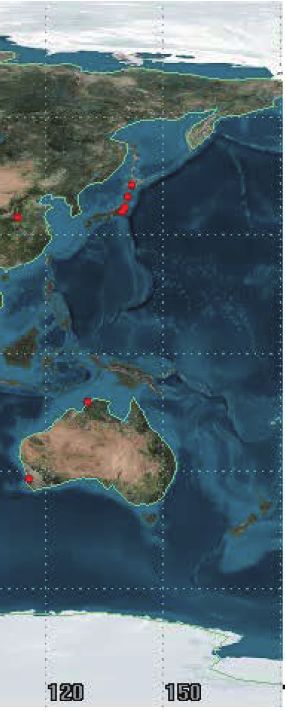
4                                                                                                                      International Journal of Aerospace Engineering

     Table 2: The minimum and the maximum revisit cycles.                                                       25

       ΔM         Minimum revisit cycle      Maximum revisit cycle

                                                                              The minimum elevation angle (o)
     (degree)           (hours)                   (hours)                                                       20

1     82.98                 3                          213
                                                                                                                15
2     115.71                27                         189
3     148.43                51                         165
                                                                                                                10
4     181.16                75                         141
5     213.89                99                         117
                                                                                                                  5
6     246.61                93                         123
7     279.34                69                         147
                                                                                                                  0
8     312.07                45                         171
9     344.80                21                         195
                                                                                                                        0       20         40         60       80
                                                                                                                                      Inclination (o)
required to cooperate with the LEO layer to realize continu-
                                                                         Figure 1: The relation between the minimum elevation angle and
ous coverage of the latitude zone including the China main-              the inclination.
land (3.86°N~53.55°N). Parameters T, W, and F can be
empirically chosen as T = 8, W = 2, and F = 1. The orbit alti-
tude and inclination are important factors affecting the
coverage rate and minimum elevation angle in this design.                                                       1.00
The higher the altitude is, the better the visibility of the com-
munication satellite is. Here the orbit altitude can be set
according to the 8-hour circular periodic orbit. As for the
                                                                          Coverage rate (o)

inclination, Figure 1 shows the relation between the mini-                                                      0.95
mum elevation angle and the inclination under the constraint
of continuous coverage. Given the requirement of a mini-
mum elevation angle higher than 20 degrees, choice of the
                                                                                                                0.90
inclination is limited between 36 and 42. Figure 2 shows the
variation of coverage rate with inclination. When inclination
is set around 40, coverage rate reaches a peak. Here the incli-
nation is set at 40, which guarantees a larger minimum eleva-                                                   0.85
tion angle and a continuous coverage at the same time. The
                                                                                                                        0        20         40         60       80
overall design configuration of the hybrid constellation is
                                                                                                                                       Inclination (o)
summarized in Table 3.
                                                                                   Figure 2: Variation of the coverage rate with the inclination.
3. Orbit Determination Scheme
This section presents the orbit determination scheme for the
                                                                                                           Table 3: Initial orbit element of the hybrid constellation.
constellation designed in Section 2, including a description of
the dynamic model, the measurement model, and the filter                                                                                       LEO layer        MEO layer
model to estimate orbit states.
                                                                         Satellite number                                                        22                8
3.1. Dynamic Model. For the constellation, the state vector is           Plane number                                                             2                2
represented as x = xT1 xT2 ⋯ xTl where xi = ri ri T , ri = rx,i          Semi-major axis (km)                                                  7189.31          20268.43
ry,i rz,i , and ri = v x,i vy,i vz,i are position and velocity vectors   Eccentricity                                                             0                0
of the satellites in J2000 Earth-centered inertial coordinate            Inclination (° )                                                       98.66              40
system. The subscripts i and l indicate the i-th satellite and           Right ascending node (° )                                          257.18/302.05        0/180
the total number of satellites, respectively. The equation of            Argument of perigee plus mean
motion for a satellite is described as                                   anomaly for the first satellite of                                     0/213.90             0/45
                                                                         every plane (° )
                            x = f x, t ,                           9

where                                                                    μ is the earth gravitational constant, and F ε represents
                                                                         perturbation accelerations. The sources of perturbations
                                     r
                                                                         include the nonspherical gravitation of the Earth (the WGS84
                   f x, t =      −μ         ,                     10
                                     r + Fε                              gravity model), the atmospheric drag (1976 standard atmo-
                                 r 3                                     sphere model), third-body perturbations (DE405 numerical
International Journal of Aerospace Engineering                                                                                      5

planetary ephemeris), solar radiation pressure (spherical           in which ru is the position of the sub-satellite point, f e is the
model), Earth radiation pressure, the tide effects, and the          flattening of the Earth, and θ is the geocentric latitude. The
effect of general relativity.                                        range to interested regions measured by the altimeter is
                                                                    expressed as
3.2. Measurement Model. In this paper, optical imagery,
altimeter data, and inter-satellite range data are used to pro-                              ρa = r − rp + ζ,                     16
vide the orientation, altitude, and relative distance informa-
tion, respectively, for the constellation satellites.
    For remote sensing satellites with an optical camera,           where rp is the position of the interested point and ζ is the
images of known ground features can be captured. By the             measurement noise which satisfies
process of image recognition and matching, the focal plane
coordinates of a ground feature are obtained, which imply                                       E ζ2 = σ2a ,                      17
the orientation information of the cameras to ground fea-
tures. The focal plane coordinates u, v satisfy
                                                                    where σa is the standard deviation of the altimeter measure-
                   u                                                ment error.
                                                                        For inter-satellite range measurement, the observed
                   f
                                                                    inter-satellite range ρs can be represented by
                                   −1
                   v   = TA TI          r − rg               11
                   f                                                                        ρs,ij = r j − ri + χ,                 18
                   1
                                                                    in which the subscripts j and i represent the j-th and i-th sat-
    TI and TA are the camera installation matrix and the            ellites, respectively, and χ presents the random measurement
rotation matrix from the satellite body coordinate frame to         noise which satisfies
the J2000 initial coordinate frame, respectively. It is assumed
that a good estimation of TA can be available from a star                                       E χ2 = σ2s                        19
tracker. f is the focal length of the optical camera, and rg is
the ground feature position. Simplifying (11) yields                   In (19), σs is the standard deviation of the inter-satellite
                                                                    range error.
                        u
                            = g x + η,                       12     3.3. Filter Model. Taking into account that the satellite orbit
                        v                                           dynamics and measurement model are nonlinear, an EKF is
                                                                    used to estimate the state of the system. Equation (9) is used
where η denotes the measurement noise satisfying the zero-          as the state equation, and (12), (15), and (18) represent the
mean Gaussian distribution                                          observation equations for different observations. The EKF
                                                                    works by a two-step cycle: a time update step and a measure-
                                                                    ment update step [23].
                       E ηηT = σ2i I2×2 ,                    13
                                                                        The covariance P propagation from time k − 1 to the next
                                                                    observation epoch k is processed with the “time update”
in which σi is the standard deviation of the focal plane coor-      equation:
dinate error and I2×2 is a two-order identity matrix.
    The laser altimeter measurement belongs to the two-                               Pk = Φ t, t k Pk−1 ΦT t, t k ,              20
way range measurement. The laser altimeter sends a laser
beam and measures the round-trip time. The range can be
                                                                    where Φ t, t k is the state transformation matrix. The state x
described as
                                                                    and covariance P are updated with the observation using the
                                                                    “measurement update” equation:
                                   ct a
                            ρa =        ,                    14
                                    2                                                                               −1
                                                                                   Kk = Pk HTk Hk Pk HTk + Rk            ,
in which c is the speed of light, t a is the round-trip time, and                   x̂k = Kk yk ,
ρa is the altimeter measurement. By adjusting the orientation                                                                     21
of the altimeter antenna boresight, the altimeter can be                            xk = xk + x̂k ,
directed toward the nadir to obtain height information above                       Pk = I − Kk Hk Pk ,
the Earth’s surface or toward interested regions to measure
the range between each other.
                                                                    where Hk is the measurement sensitivity matrix which is the
    When the altimeter is directed toward the nadir, the
                                                                    partial derivative of measurements with respect to the state
range measurement is described as
                                                                    vector, Kk is the gain matrix, x̂k is the state deviation, and
                                                                    y k is the observation residual. The measurement sensitivity
         ρa = r − ru + ζ = r − re 1 − f e sin2 θ + ζ,        15     matrixes can be derived according to the observation
6 International Journal of Aerospace Engineering
equations. For different measurement models, the measure-
ment sensitivity matrixes can be expressed as follows:
For image measurement (the detailed formula is in
Appendix B),
∂ u, v
Hik = 22
∂r
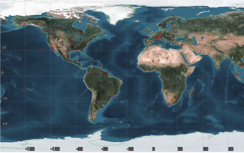
For the altimeter measurement to interested regions, Figure 3: The distribution of the geometric calibration sites on the
T
Earth’s surface.
r − rp
Hak = 01×3 23
r − rp
achieved by satellites. The probability that the imaged region
is covered by clouds is set as 50%. Measurement errors from
For altimeter measurement toward the nadir, different sources were simulated by Gaussian zero-mean ran-
dom error for three measurement data. The uncertainty of
r x 2r e f e r x r 2z ry 2r e f e r y r 2z rz inter-satellite range was set as 1 m (1σ). For optical imagery,
Hak = − − the measurement error of focal plane coordinates mainly
r r4 r r r
results from three sources: the image resolution was set as
24 1 m (1σ), the pointing accuracy was chosen as 0.001° , and
2r e f e r z r2x + r 2y the coastline and rivers were used as ground features with a
− 01×3 10 m (1σ) position error [8]. For the altimeter data, although
r
the altimeter precision can reach the level of centimeters, the
height measuring accuracy used in orbit determination is also
For inter-satellite range measurement (the homologous influenced by several other factors. For example, the differ-
part of one satellite in the link), ence between the actual Earth ground and the geodetic refer-
ence ellipsoid is the main factor leading to the height
r − ri T measurement error [23]. Besides, due to beam divergence,
Hsk = 01×3 25 the altimeter range measurement is the average of the ranges
r − ri
from the altimeter to the footprint of each laser beam on the
Earth surface. The effect of this averaging could be decreased
Once a new observation is obtained, the state is updated.
when only ocean altimeter data is used, as ocean topography
The updated state is propagated forward to the next obser-
is flatter than that of land. Considering these facts, a 10 m
vation time, and the filter continues until all measurements
(1σ) error was added to ocean altimeter data with the help
are processed.
of the precise Earth shape and tide model. Unlike the tradi-
tional usage pattern of the altimeter, a laser altimeter can be
4. Simulation Results used to measure the range between satellites and some
In the section, orbit determination performance of simula- interested regions when used in combination with optical
tions using different strategies for the hybrid constellation cameras. This is achieved by making the laser altimeter
are evaluated and compared. point to the ground features that can be captured and rec-
ognized by optical cameras. The geometer calibration sites
4.1. Initial Condition. The initialization was set at the epoch applied in mission SPOT6 and provided by ESA [24] were
(1 July 2009, 10:30:00), and the initial orbit elements are used as the ground targets in this paper. The site distribu-
shown in Table 3. Nominal orbit data of the hybrid constel- tion is shown in Figure 3. The small number of ground sites
lation was generated considering all perturbations referred would make it hard to capture them. Therefore, it is
to in Section 3.1. The dynamic model used in orbit determi- assumed that the satellites can swing (the swing angle is
nation includes (1) the two-body gravitation, (2) the non- no more than 30° ) to point to these sites, when approaching
spherical gravitation (the WGS84 20 × 20 gravity), (3) the them. In such a situation, the altimeter measurement error
atmospheric perturbation (1976 standard atmosphere model), was set as 1 m (1σ).
(4) the gravitation of the Moon and Sun (DE405 numerical In these scenarios, all measurements were obtained with
planetary ephemeris), (5) the solar radiation pressure (spher- an interval of 1 min. The inter-satellite range data and altim-
ical model), and (6) the perturbation of rigid tides. eter data are generated by the nominal orbit data and Refer-
For MEO layer satellites, only inter-satellite range data ence Earth Model (WGS84). Due to the use of synthetic data
can be used to determine orbit, while for LEO layer satellites, instead of real satellite imagery, the image processing stage is
the inter-satellite range data, optical imagery, and altimeter not considered in this article. Thus, related latency is not
data can all be used to determine orbit. The visibility limitation involved in the simulations. The observed coordinates of
was taken into consideration while generating inter-satellite ground features on the focal plane are generated through
range data. For optical imagery, when the sub-satellite region geometric relationships between the positions of ground fea-
is at night or covered by clouds, no effective images can be tures and the actual orbit, under the nadir imaging model.
International Journal of Aerospace Engineering                                                                                                        7

                             100

                                                                                   x-direction (cm s−1)
       in x-direction (m)                                                                                  10

                                                                                     Velocity error in
                              50
         Position error

                               0                                                                            0

                            −50
                                                                                                          −10
                            −100
                                   0.0         0.5           1.0       1.5   2.0                                0.0   0.5       1.0       1.5   2.0

                                                                                   y-direction (cm s−1)
       in y-direction (m)

                             100                                                                           10

                                                                                     Velocity error in
         Position error

                               0                                                                            0

                            −100                                                                          −10

                                   0.0         0.5           1.0       1.5   2.0                                0.0   0.5       1.0       1.5   2.0

                                                                                   z-direction (cm s−1)
       in z-direction (m)

                             100                                                                           20
                                                                                     Velocity error in
         Position error

                               0                                                                            0

                            −100                                                                          −20

                                   0.0         0.5          1.0        1.5   2.0                                0.0   0.5      1.0        1.5   2.0
                                                         Time (days)                                                        Time (days)
                                         3휎 standard deviation
                                         State error

Figure 4: Time history of position and velocity errors of a LEO layer satellite in the J2000 coordinate frame for the case using only optical
imagery.

For the satellite orbit, the initial position error was 100 m and                       RMS errors increase by a factor of 2.30 for position error
the initial velocity error was set as 0.1 cm/s.                                         and 1.90 for velocity error. In general, the EKF should be able
                                                                                        to filter out measurements characterized by higher error;
4.2. Results and Analysis. In this part, results of case simula-                        thus, the orbit determination accuracy would not decrease
tions using different orbit determination strategies are ana-                            when more measurements are added to an EKF. However,
lyzed in detail.                                                                        the result draws the opposite conclusion in this simulation.
    The comparison was first conducted between the case                                  This is mainly due to the small amount of valid images.
using only optical imagery and the case using either altimeter                          Although the optical imagery is set to be captured at a high
data. As the orbit determination results are similar for all                            frequency with an interval of 1 min, only a small fraction of
LEO layer satellites under these two scenarios, only results                            the images that contain a ground feature can be used as valid
of the first satellite in the LEO layer are shown. Figure 4                              observation. Factors including small FOV, the discontinued
shows the time history of orbit error only using optical imag-                          distribution of the ground feature, and existence of light con-
ery, and the orbit determination results using optical imagery                          straints would lead to the absence of a ground feature in some
and altimeter data as inputs are presented in Figures 5 and 6.                          images and result in a lower measurement frequency of valid
In these figures, the black line in each plot denotes the actual                         imagery compared to that of the ocean altimeter data. What
orbit error, and the red line indicates the 3σ standard devia-                          is more, the ocean altimeter data only provides radial mea-
tion of the estimated error. It can been seen that for all cases,                       surement and is not precise enough. Therefore, the orbit pre-
the actual errors are well-bounded by the 3-sigma standard                              cision decreases when the ocean altimeter data is added. On
deviations and drop significantly to a steady state in less than                         the contrary, in the case using altimeter data pointing to
0.2 days. Because the measurement and dynamic model are                                 the geometer calibration sites and optical imagery, a better
nonlinear, a Monte Carlo test of 100 runs was performed to                              performance than the case using only optical imagery is
further compare orbit determination accuracy, and the aver-                             achieved, with a 41.35% enhancement in position accuracy
age RMS errors are given in Table 4. In the case using ocean                            and 45.14% enhancement in velocity accuracy.
altimeter data and optical imagery, the results get worse com-                              In the case using optical imagery, altimeter data, and
pared with the case using only optical imagery. The average                             inter-satellite range data, the orbits of both LEO layer
8                                                                                                                     International Journal of Aerospace Engineering

                             600                                                                           60

                                                                                   x-direction (cm s−1)
       in x-direction (m)

                                                                                     Velocity error in
                             300                                                                           30
         Position error

                               0                                                                            0

                            −300                                                                          −30

                            −600                                                                          −60
                                   0.0         0.5           1.0       1.5   2.0                                0.0        0.5        1.0        1.5       2.0
                                                              A                                                                       A
                             400                                                                           40

                                                                                   y-direction (cm s−1)
       in y-direction (m)

                                                                                     Velocity error in
                             200                                                                           20
         Position error

                               0                                                                            0

                            −200                                                                          −20

                            −400                                                                          −40
                                   0.0         0.5           1.0       1.5   2.0                                0.0        0.5        1.0        1.5       2.0
                                                              A                                                                        A
                             400                                                                           40

                                                                                   z-direction (cm s−1)
       in z-direction (m)

                             200                                                     Velocity error in
         Position error

                                                                                                           20

                               0                                                                            0

                            −200                                                                          −20

                            −400                                                                          −40
                                   0.0         0.5          1.0        1.5   2.0                                0.0        0.5       1.0         1.5       2.0
                                                         Time (days)                                                              Time (days)
                                         3휎 standard deviation
                                         State error

Figure 5: Time history of position and velocity errors of a LEO layer satellite in the J2000 coordinate frame for the case using optical imagery
and ocean altimeter data.

satellites and MEO layer satellites can be determined simulta-                          generate effective remote sensing observations. Thus, another
neously with the help of inter-satellite range data. The time                           two scenarios where there is a lack of remote sensing obser-
history of orbit errors for a LEO satellite and a MEO satellite                         vation for certain LEO layer satellites are discussed. One (sce-
is show in Figures 7 and 8. It is obvious that the position error                       nario 1) assumes that satellites on the first plane of the LEO
and velocity error further decrease compared with the cases                             layer fail to obtain altimeter measurement while other LEO
discussed before. This conclusion is also confirmed by results                           satellites can get all three measurement data. The other (sce-
from the Monte Carlo runs in Table 4. The average RMS                                   nario 2) assumes that the satellites on the first plane of the
errors of position and velocity drop to 47.24% and 42.70%,                              LEO layer fail to obtain both imagery and altimeter data
respectively, compared to those in the case using optical                               while other satellites can get all three measurement data.
imagery and altimeter data. The improvement in orbit accu-                              The same Monte Carlo runs were applied to these two sce-
racy can be explained as follows: to the multiplane, multilayer                         narios, and simulated results are compared with the ideal
structure of the hybrid constellation, a good geometry config-                           case mentioned above in which all satellites in the LEO layer
uration for relative range measurement is established. Under                            can obtain three measurement data. As is shown in Table 5,
this configuration, the high-precision inter-satellite range                             for the same scenario, there is no significant difference on
data can effectively improve orbit determination accuracy                                the orbit accuracy between LEO satellites with and without
in all directions.                                                                      a loss of remote sensing observation. Taking scenario 1 as
     In the above-mentioned case, all three data including                              an example, the change of position error (from 9.03 to
optical imagery, altimeter data, and inter-satellite range data                         9.05) and velocity error (from 0.94 to 0.94) is almost negligi-
are used for orbit determination. However, in actual mis-                               ble. However, between different scenarios, there exists signif-
sions, the remote sensing instruments may have malfunction                              icant difference on the average RMS of position and velocity
or get disturbed, and there are circumstances that LEO layer                            errors. As long as there is absence of remote sensing observa-
satellites are not loaded with both optical cameras and altim-                          tions, the orbit determination precisions for all satellites in
eters due to their mission requirements. These situations                               the hybrid constellation decline significantly compared to
would make it impossible for certain LEO layer satellites to                            the ideal scenario.
International Journal of Aerospace Engineering                                                                                                                            9

                             100                                                                                    20

                                                                                            x-direction (cm s−1)
       in x-direction (m)

                                                                                              Velocity error in
                              50                                                                                    10
         Position error

                               0                                                                                     0

                            −50                                                                                    −10

                            −100                                                                                   −20
                                   0.0            0.5           1.0       1.5         2.0                                0.0   0.5          1.0              1.5   2.0

                                                                                                                    10

                                                                                            y-direction (cm s−1)
                             100
       in y-direction (m)

                                                                                              Velocity error in
                                                                                                                     5
         Position error

                               0                                                                                     0

                                                                                                                   −5
                            −100
                                                                                                                   −10
                                   0.0            0.5           1.0       1.5         2.0                                0.0   0.5          1.0              1.5   2.0

                                                                                            z-direction (cm s−1)
       in z-direction (m)

                              50                                                                                    10
                                                                                              Velocity error in
         Position error

                               0                                                                                     0

                            −50                                                                                    −10

                                   0.0            0.5          1.0        1.5         2.0                                0.0   0.5         1.0               1.5   2.0
                                                            Time (days)                                                                 Time (days)
                                            3휎 standard deviation
                                            State error

Figure 6: Time history of position and velocity errors of a LEO layer satellite in the J2000 coordinate frame for the case using optical imagery
and range data to the geometric calibration sites.

                                         Table 4: Average RMS errors of 100 Monte Carlo runs for different orbit determination scenarios.

                                                                                                                                 RMS error
                                                                                                             LEO layer satellite           MEO layer satellite
                                                                                                      Position (m) Velocity (cm/s) Position (m) Velocity (cm/s)
Image                                                                                                              14.22         1.75                  —            —
Image + altimeter (ocean)                                                                                          32.77         3.32                  —            —
Image + altimeter (the geometer calibration site)                                                                  8.34          0.96                  —            —
Image + altimeter (the geometer calibration site) + inter-satellite range                                          3.94          0.41                 9.06         0.38

5. Conclusions                                                                                   MEO layer is designed in conjunction with the LEO layer
                                                                                                 for communication and is capable of providing continuous
In this paper, we proposed an autonomous orbit determina-                                        coverage of latitude zone including China mainland.
tion scheme for hybrid constellations by using a combination                                         With the help of measurement from onboard optical
of three measurement data including optical imagery, altim-                                      cameras and altimeters, orbits of individual LEO satellites
eter data, and inter-satellite range data. By applying the                                       can be autonomously determined. Comparison results show
scheme to a constructed hybrid constellation, the perfor-                                        that a better performance is achieved when optical imagery
mance of the scheme is then investigated. The hybrid constel-                                    is used in combination with altimeter data pointing to the
lation consists of satellites in two LEO/MEO layers. The LEO                                     geometer calibration sites than with ocean altimeter data.
layer is designed for Earth observation, which is capable of                                     For MEO satellites, orbits can be determined autonomously
providing complete coverage of the Earth (except polar                                           by considering inter-satellite range data in combination with
regions) and has a maximum revisit cycle of 117 hours. The                                       remote sensing observations, which in turn lead to a further
10 International Journal of Aerospace Engineering
20
x-direction (cm s−1)
in x-direction (m)
Velocity error in
2
Position error
10
0 0
−10
−2
−20
0.0 0.5 1.0 1.5 2.0 0.0 0.5 1.0 1.5 2.0
y-direction (cm s−1)
in y-direction (m)
Velocity error in
10 2
Position error
0 0
−10 −2
0.0 0.5 1.0 1.5 2.0 0.0 0.5 1.0 1.5 2.0
z-direction (cm s−1)
in z-direction (m)
Velocity error in
10 2
Position error
0 0
−10 −2
0.0 0.5 1.0 1.5 2.0 0.0 0.5 1.0 1.5 2.0
Time (days) Time (days)
3휎 standard deviation
State error
Figure 7: Time history of position and velocity errors of a LEO layer satellite in the J2000 coordinate frame for the case using all three
observation data.
60
x-direction (cm s−1)
40
in x-direction (m)
Velocity error in
Position error
20 30
0 0
−20 −30
−40
−60
0.0 0.5 1.0 1.5 2.0 0.0 0.5 1.0 1.5 2.0
y-direction (cm s−1)
40 40
in y-direction (m)
Velocity error in
Position error
20 20
0 0
−20 −20
−40 −40
0.0 0.5 1.0 1.5 2.0 0.0 0.5 1.0 1.5 2.0
40 60
z-direction (cm s−1)
in z-direction (m)
Velocity error in
Position error
20 30
0 0
−20 −30
−40 −60
0.0 0.5 1.0 1.5 2.0 0.0 0.5 1.0 1.5 2.0
Time (days) Time (days)
3휎 standard deviation
State error
Figure 8: Time history of position and velocity errors of a MEO layer satellite in the J2000 coordinate frame for the case using all three
observation data.International Journal of Aerospace Engineering 11
Table 5: Average RMS errors of 100 Monte Carlo runs for the scenarios losing certain remote sensing observation.
RMS error
LEO layer
Satellites without a loss of remote Satellites with a loss of remote MEO layer
sensing observations sensing observations
Position (m) Velocity (cm/s) Position (m) Velocity (cm/s) Position (m) Velocity (cm/s)
Ideal scenario 3.94 0.41 — — 9.06 0.38
Scenario 1 9.03 0.94 9.05 0.94 25.29 0.66
Scenario 2 11.14 1.15 11.12 1.15 35.42 0.83
improvement of orbit accuracy for LEO satellites. To center to the connection line of two adjacent satellites should
approach real-world simulations, we investigated the orbit be larger than the Earth radius. The corresponding mathe-
determination performance in situations where certain matical expression is
remote sensing observations are absent. Two scenarios in
which only altimeter data or both imagery and altimeter data φ r
≤ arccos e , A2
are absent on half of the LEO satellites are considered. Results 2 a
show that compared to the ideal scenario, orbit determina-
tion performance of the hybrid constellation declines in both in which φ is the geocentric angle between two adjacent
scenarios. However, for each scenario, orbit precision satellites. As there are Ns satellites in an orbit plane, the geo-
between LEO satellites with and without lack of measure- centric angle can be given as
ments shows no difference. These results provide a reference
2π
for autonomous operation of constellations containing φ= A3
remote sensing satellites and communication satellites in Ns
future missions.
In the paper, the design of the constellation is based Substituting (A.3) into (A.2) and considering that the num-
mainly on experience and deterministic algorithm. When ber of satellites required is no larger than 2 times this minimum
more constraints are considered or more parameters need number, the third inequality relation in (7) can be obtained:
to be optimized, a heuristic algorithm could be used instead.
π 2π
Additionally, in order to further improve radial orbit accu- ≤ Ns ≤ A4
racy, the altimeter crossover data could be used. How these arccos re /a arccos r e /a
changes would influence the orbit determination perfor-
mance is worthy of in-depth analysis in future work. The fourth constraint is that the single-plane constellation
can provide complete coverage of the Earth (except polar
regions). For analyzing the coverage of satellites, the swath
Appendix width W s of a satellite needs to be known, which is
A. The Derivation of (7)
FOV
W s = 2 a − re tan A5
The expression of equation (7) is 2
N d ≤ 10, With (A.5), the width for every satellite sweep on the equa-
tor is
Np
14 ≤ ≤ 15, Ws
Nd We = A6
sin i
π 2π
≤ Ns ≤ ,
arccos r e /a arccos re /a Since the equator is the longest latitude circle, the complete
2 a − re tan FOV/2 Nd coverage of the Earth (except polar regions) is equivalent with
> 2πr e the complete coverage of the equator region. Thus, in a revisit
sin i LCM N d , N s N p
period, the constraint condition that satellites on an orbit plane
A1 can provide complete coverage of the Earth can be expressed as
The first two mathematical formulations in (7) are com- LCM N d , N s N p
W e > 2πr e , A7
prehensible, which present the constraints: the revisit cycle is Nd
less than 10 days and the orbit revolution per day is more
than 14 and less than 15. where LCM N d , N s represents the least common multiple of
For the third constraint, in order to make sure that it is N d and N s . Substituting (A.5) and (A.6) into (A.7) yields the
visible between adjacent satellites, the distance of the Earth fourth inequality relation in (7).12 International Journal of Aerospace Engineering
B. The Detailed Formula of (22)
The detailed formula of equation (22) is ( a11 , … , a33 are
elements of TA TI −1 )
g g g g g g
a31 a12 − a11 a32 ry − ry + a31 a13 − a11 a33 r z − rz a32 a12 − a12 a31 r x − r x + a32 a13 − a11 a33 rz − rz a33 a11 − a13 a31 r x − r x + a32 a13 − a12 a33 ry − r y
−f g g g 2
−f g g g 2
−f g g g 2
0 1×3
a31 rx − r x + a32 ry − r y + a33 r z − rz a31 rx − rx + a32 r y − ry + a33 rz − r z a31 rx − rx + a32 ry − r y + a33 rz − rz
Hik = g g g g g g
a31 a22 − a21 a32 ry − ry+ a31 a23 − a21 a33 r z − rz a32 a22 − a22 a31 rx − rx + a32 a23 − a21 a33 rz − rz a33 a21 − a23 a31 rx − rx + a32 a23 − a22 a33 ry − r y
−f g g g 2
−f g g g 2
−f g g g 2
0 1×3
a31 rx − r x + a32 ry − r y + a33 r z − rz a31 rx − rx + a32 r y − ry + a33 rz − r z a31 rx − rx + a32 ry − r y + a33 rz − rz
A8
Data Availability [6] R. L. White, M. B. Adams, E. G. Geisler, and F. D. Grant, “Atti-
tude and oribit estimation using stars and landmarks,” IEEE
The data used to support the findings of this study are avail- Transactions on Aerospace and Electronic Systems, vol. AES-
able from the corresponding author upon request. 11, no. 2, pp. 195–203, 1975.
[7] M. Straub and J. Christian, “Autonomous optical navigation
for Earth-observing satellites using coastline matching,” in
Conflicts of Interest AIAA Guidance, Navigation, and Control Conference, Kissim-
The authors declare that there is no conflict of interest mee, FL, USA, 2015.
regarding the publication of this paper. [8] M. Li, B. Xu, and L. Zhang, “Orbit determination for remote-
sensing satellites using only optical imagery,” International
Journal of Remote Sensing, vol. 38, no. 5, pp. 1350–1364, 2017.
Acknowledgments [9] M. Li and B. Xu, “Autonomous orbit and attitude determina-
tion for Earth satellites using images of regular-shaped ground
This work was carried out with financial support from objects,” Aerospace Science and Technology, vol. 80, pp. 192–
the National Basic Research Program 973 of China 202, 2018.
(2015CB857100), the Base of National Defence Scientific [10] G. H. Born, B. D. Tapley, and M. L. Santee, “Orbit determina-
Research Fund (Nos. 2016110C019 and JCKY2016203C067), tion using dual crossing arc altimetry,” Acta Astronautica,
and the National Natural Science Foundation (No. 11603011). vol. 13, no. 4, pp. 157–163, 1986.
[11] F. G. Lemoine, D. D. Rowlands, S. B. Luthcke et al., “Precise
References orbit determination for Geosat follow-on using satellite laser
ranging data and intermission altimeter crossovers,” in 2001
[1] A. L. Jennings and H. Diniz, “Global navigation satellite Flight Mechanics Symposium, Greenbelt, MD, USA, 2001.
system design exploration using a multi-objective genetic algo- [12] F. Markley and U. Naval, “Autonomous navigation using land-
rithm,” in AIAA SPACE 2015 Conference and Exposition, mark and intersatellite data,” in AIAA/AAS Astrodynamics
p. 4622, Pasadena, CA, USA, 2015. Conference, Seattle, WA, USA, 1984.
[2] H. Xu, X. Zhang, and X. Zhan, “Analyzing RAIM performance [13] M. L. Psiaki, “Autonomous orbit determination for two space-
for an MEO/GEO hybrid GNSS constellation,” in IET Interna- craft from relative position measurements,” Journal of Guid-
tional Communication Conference on Wireless Mobile and ance, Control, and Dynamics, vol. 22, no. 2, pp. 305–312, 1999.
Computing (CCWMC 2011), pp. 465–467, Shanghai, China,
[14] R. Li, H. Qiu, and K. Xiong, “Autonomous navigation for con-
November 2011.
stellation based on inter-satellite ranging and directions,” in
[3] S. Chan, A. T. Samuels, N. B. Shah, J. E. Underwood, and O. L. IECON 2017 - 43rd Annual Conference of the IEEE Industrial
De Weck, “Optimization of hybrid satellite constellations Electronics Society, pp. 2985–2990, Beijing, China, November
using multiple layers and mixed circular-elliptical orbits,” in 2017.
22nd AIAA International Communications Satellite Systems
[15] X. Kai, W. Chunling, and L. Liangdong, “Autonomous naviga-
Conference & Exhibit 2004, pp. 9–12, Monterey, CA, USA,
tion for a group of satellites with star sensors and inter-satellite
May 2004.
links,” Acta Astronautica, vol. 86, pp. 10–23, 2013.
[4] M. Luglio and W. Pietroni, “Optimization of double-link
transmission in case of hybrid orbit satellite constellations,” [16] X. Kai, W. Chunling, and L. Liangdong, “The use of X-ray
Journal of Spacecraft and Rockets, vol. 39, no. 5, pp. 761–770, pulsars for aiding navigation of satellites in constellations,”
2002. Acta Astronautica, vol. 64, no. 4, pp. 427–436, 2009.
[5] E. Fahnestock and R. S. Erwin, “Optimization of hybrid satel- [17] S. Wang and P. Cui, “Autonomous orbit determination using
lite and constellation design for GEO-belt space situational pulsars and inter-satellite ranging for Mars orbiters,” in 2018
awareness using genetic algorithms,” in Proceedings of the IEEE Aerospace Conference, Big Sky, MT, USA, March 2018.
2005, American Control Conference, 2005, pp. 2110–2115, [18] M. Capderou, Handbook of Satellite Orbits: From Kepler to
Portland, OR, USA, June 2005. GPS, Springer Science & Business, 2014.International Journal of Aerospace Engineering 13
[19] https://directory.eoportal.org/web/eoportal/satellite-missions/
d/dmc-3.
[20] D. Mortari, M. P. Wilkins, and C. Bruccoleri, “The Flower
Constellations,” Journal of Astronautical Sciences, vol. 52,
pp. 107–127, 2004.
[21] M. P. Wilkins and D. Mortari, “Flower Constellation set theory
part ii: secondary paths and equivalency,” IEEE Transactions
on Aerospace and Electronic Systems, vol. 44, no. 3, pp. 964–
976, 2008.
[22] J. G. Walker, Continuous Whole-Earth Coverage by Circular-
Orbit Satellite Patterns, Royal Aircraft Establishment
Farnborough (United Kingdom), 1977.
[23] B. Schutz, B. Tapley, and G. H. Born, Statistical Orbit Determi-
nation, Academic Press, 2004.
[24] http://calvalportal.ceos.org/calibration-test-sites.International Journal of
Rotating Advances in
Machinery Multimedia
The Scientific
Engineering
Journal of
Journal of
Hindawi
World Journal
Hindawi Publishing Corporation Hindawi
Sensors
Hindawi Hindawi
www.hindawi.com Volume 2018 http://www.hindawi.com
www.hindawi.com Volume 2018
2013 www.hindawi.com Volume 2018 www.hindawi.com Volume 2018 www.hindawi.com Volume 2018
Journal of
Control Science
and Engineering
Advances in
Civil Engineering
Hindawi Hindawi
www.hindawi.com Volume 2018 www.hindawi.com Volume 2018
Submit your manuscripts at
www.hindawi.com
Journal of
Journal of Electrical and Computer
Robotics
Hindawi
Engineering
Hindawi
www.hindawi.com Volume 2018 www.hindawi.com Volume 2018
VLSI Design
Advances in
OptoElectronics
International Journal of
International Journal of
Modelling &
Simulation
Aerospace
Hindawi Volume 2018
Navigation and
Observation
Hindawi
www.hindawi.com Volume 2018
in Engineering
Hindawi
www.hindawi.com Volume 2018
Engineering
Hindawi
www.hindawi.com Volume 2018
Hindawi
www.hindawi.com www.hindawi.com Volume 2018
International Journal of
International Journal of Antennas and Active and Passive Advances in
Chemical Engineering Propagation Electronic Components Shock and Vibration Acoustics and Vibration
Hindawi Hindawi Hindawi Hindawi Hindawi
www.hindawi.com Volume 2018 www.hindawi.com Volume 2018 www.hindawi.com Volume 2018 www.hindawi.com Volume 2018 www.hindawi.com Volume 2018You can also read