A Fractal Model of Hydraulic Conductivity for Saturated Frozen Soil - MDPI
←
→
Page content transcription
If your browser does not render page correctly, please read the page content below
water
Article
A Fractal Model of Hydraulic Conductivity for
Saturated Frozen Soil
Lei Chen 1,2 , Dongqing Li 1 , Feng Ming 1, *, Xiangyang Shi 1,2 and Xin Chen 1,2
 1   State Key Laboratory of Frozen Soil Engineering, Northwest Institute of Eco-Environment and Resources,
     Chinese Academy of Sciences, Lanzhou 730000, China; ChenLei8@lzb.ac.cn (L.C.); dqli@lzb.ac.cn (D.L.);
     shixiangyang2008@163.com (X.S.); chenxcumt@sina.com (X.C.)
 2   University of Chinese Academy of Sciences, Beijing 100049, China
 *   Correspondence: mingfeng05@lzb.ac.cn; Tel.: +86-93-1496-7469

 Received: 10 December 2018; Accepted: 18 February 2019; Published: 21 February 2019

 Abstract: In cold regions, hydraulic conductivity is a critical parameter for determining the water
 flow in frozen soil. Previous studies have shown that hydraulic conductivity hinges on the pore
 structure, which is often depicted as the pore size and porosity. However, these two parameters do not
 sufficiently represent the pore structure. To enhance the characterization ability of the pore structure,
 this study introduced fractal theory to investigate the influence of pore structure on hydraulic
 conductivity. In this study, the pores were conceptualized as a bundle of tortuous capillaries with
 different radii and the cumulative pore size distribution of the capillaries was considered to satisfy
 the fractal law. Using the Hagen-Poiseuille equation, a fractal capillary bundle model of hydraulic
 conductivity for saturated frozen soil was developed. The model validity was evaluated using
 experimental data and by comparison with previous models. The results showed that the model
 performed well for frozen soil. The model showed that hydraulic conductivity was related to the
 maximum pore size, pore size dimension, porosity and tortuosity. Of all these parameters, pore size
 played a key role in affecting hydraulic conductivity. The pore size dimension was found to decrease
 linearly with temperature, the maximum pore size decreased with temperature and the tortuosity
 increased with temperature. The model could be used to predict the hydraulic conductivity of frozen
 soil, revealing the mechanism of change in hydraulic conductivity with temperature. In addition,
 the pore size distribution was approximately estimated using the soil freezing curve, making this
 method could be an alternative to the mercury intrusion test, which has difficult maneuverability
 and high costs. Darcy’s law is valid in saturated frozen silt, clayed silt and clay, but may not be valid
 in saturated frozen sand and unsaturated frozen soil.

 Keywords: frozen soil; soil freezing curve; hydraulic conductivity; fractal model; Darcy’s law

1. Introduction
     Hydrology in cold regions is a rapidly progressing research field, representing an important
sub-discipline of hydrology. Recently, research interest in cold region hydrology has been spurred
by global warming-induced hydrological and ecological changes to cold regions, such as permafrost
degradation, glacial recession and surface runoff shrinkage [1]. Cold region hydrology includes
permafrost hydrology, glacier hydrology and snow hydrology, of which permafrost hydrology is
the broader scientific field owing to permafrost’s wide distribution, covering about a quarter of the
land surface of the world [2]. Frozen soil is a special type of soil-water system composed of soil
particles, liquid water, ice and gas. The emergence and existence of ice changes the driving force of
water migration, leading to changes in migration direction, migration distance, migration velocity and
migration amount; these produce further changes in the water distribution in frozen soil. Previously,

Water 2019, 11, 369; doi:10.3390/w11020369                                      www.mdpi.com/journal/water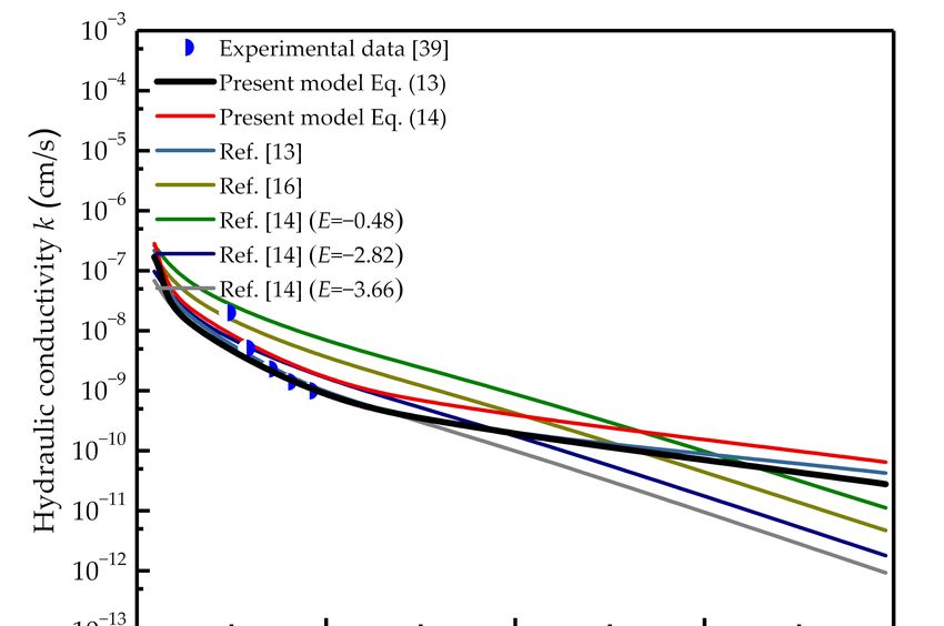
Water 2019, 11, 369                                                                               2 of 20

frozen soil has often been conceptualized as an impermeable barrier that inhibits infiltration and
promotes surface and near-surface runoff; however, researchers have since investigated the hydraulic
conductivity of frozen soil and found that frozen soil is not a complete aquiclude, as liquid water
could migrate in the frozen soil. Thus, water migration in frozen soil is one of the main processes in
permafrost hydrology. Due to the free energy of soil particles and water-air interfaces, some water in
frozen soil remains unfrozen at sub-zero temperatures [3]—defined as unfrozen water. The unfrozen
water will flow along a temperature gradient or pressure gradient, resulting in water and solute
redistribution [4], frost heaving [5], and salt expansion [6]. Such damage causes problems during the
construction of engineering ground structures in cold regions, including roads, railways, pipelines,
buildings and dams. In frozen soil, at least in high-temperature frozen soil, the unfrozen water
transported in the frozen soil is always assumed to follow Darcy’s law:

                                                       ∆H
                                              V = kf                                                 (1)
                                                        L
where V is Darcy’s flux (m/s); kf is the hydraulic conductivity of frozen soil (m/s); ∆H is the water
head loss between two cross sections (m), ∆H = H1 − H2 , where H is the total head (m), defined as
the sum of the elevation head Z and the pressure head hw ; and L is the distance of the seepage path
between these two cross sections (m). As Equation (1) shows, hydraulic conductivity is one of the key
parameters for determining water flow in frozen soil.
      To further predict water redistribution, frost heave and salt expansion, several hydrology and
hydrogeology models had been developed by coupling a groundwater flow equation with heat transfer
equations. Researchers applying these mathematical models are faced with difficulties due to a lack
of precise values of hydraulic conductivity. The main reason for this deficiency is that measuring
the hydraulic conductivity of frozen soil remains difficult and a complete expression for hydraulic
conductivity is not yet available. This problem leads to a general assumption being made that the
hydraulic conductivity of frozen soil is, in most cases, zero. However, it has been found in most of the
studies that water flow still occurs in frozen soil, especially in high-temperature frozen soil, making
this assumption unreasonable. The main objective of this paper is to provide a solution to this problem
by presenting a new mathematical model for estimating the hydraulic conductivity of saturated frozen
soil with a limited set of data.

2. Background
      Many attempts have been undertaken to determine the hydraulic conductivity of frozen soil.
Burt and Williams [7] measured saturated hydraulic conductivity using a permeameter. In this study,
water was used as the fluid. To prevent the water from melting the frozen soil, lactose was added
to ensure that the fluid was in thermodynamic equilibrium with the water in the soil. In addition,
the lactose had restricted entry to the soil through the use of a dialysis membrane. In other studies,
to solve the problem of the water melting the frozen soil, different fluids other than water have
been used to measure hydraulic conductivity; for example, Horiguchi and Miller [8] used distilled
water; Wiggert et al. [9] used dacane, octane, heptane and NaCl brine; McCauley et al. [10] used
diesel; and Seyfried and Murdock [11] used air. All of these studies tended to overestimate hydraulic
conductivity because the fluids could flow due to air-filled porosity, making it difficult to obtain an
accurate hydraulic conductivity measuring by such experiments alone.
      Many mathematical models for predicting the hydraulic conductivity of frozen soil have since
been recommended. These mathematical models include empirical models and statistical models.
For empirical models, there are three main types. The first type is determined by the assumption that
the hydraulic conductivity of frozen soil is a function of temperature. For the convenient application
in numerical models, Horiguchi and Miller [12] gave an empirical formula, kf = C × T D , where,
kf is the hydraulic conductivity of frozen soil (m/s), T is the temperature (◦ C), and C and D are
constant fitting parameters. Nixon [13] proposed a similar temperature-dependent empirical formula
Water 2019, 11, 369                                                                                                              3 of 20

as follows, kf = k0 /(− T )δ , where, k0 is the hydraulic conductivity at −1 ◦ C and δ is the slope of the
kf − T relationship in a log-log coordinate; however, these models must be determined using some
type of experimental data, thus limiting their applicability. The second type of empirical model is
determined by the assumption that the ice in saturated frozen soil and the air in unsaturated unfrozen
soil plays a similar role in the process of water seepage when there is the same water content; that is the
hydraulic conductivity of saturated frozen soil is closed to that of unsaturated melted soil. A drawback
of this model is that it always overrates the hydraulic conductivity of frozen soil. The third model
type is determined by the fact that the second model overestimates the hydraulic conductivity of
frozen soil, resulting in an ice impedance being introduced. Jame and Norum [14] introduced an
impedance factor, kf = ku /10− Eθi , where, ku is the hydraulic conductivity of unfrozen soil with the
same liquid water content (m/s), E is an empirical constant and, θi is the volumetric content of ice
(m3 /m3 ). Based on agreement with experimental data from Jame and Norum [14] and Burt and
Williams [7], Taylor and Luthin [15] gave a specific impedance factor, kf = ku /1010θi . Mao et al. [16]
presented another impedance factor form to express hydraulic conductivity, kf = ku × (1 − θi )3 ;
however, many researchers have criticized this model because of the arbitrary choice of impedance
factor. Shang et al. [17] suggested that the impedance factor would be better determined using
I = kf /ku ; however, this method is still limited by a paucity of the measured data and, moreover, the
impedance factor is not a constant.
      Meanwhile, several statistical models have also been proposed, of which there are two main types.
The first type of statistical model is determined by the capillary bundle model and the Hagen-Poiseuille
equation. Watanabe and Flury [18] developed a new capillary bundle model, in which the ice is
assumed to form in the centre of the capillaries, leaving a circular annulus open for liquid water
flow. On this premise, a newly developed hydraulic conductivity model was suggested, as seen in
Equation (2):
                                        "                     2 #
                                      M                                       R J 2 −ri J 2
                                      ∑ n J R J 4 − ri J 4 +
                             γw π
                      kf =   8µτ
                                                                                                    R J − d ( T ) ≥ ri ( T )
                                    J = k +1                                 ln ri J /R J
                                                                                                                                    (2)
                                                          M
                                                          ∑ nJ RJ4
                                               γw π
                                      kf =     8µτ                                 R J − d ( T ) < ri ( T )
                                                      J = k +1

where, n J is the number of capillaries of radius R J per unit area; ri J is the radius of cylindrical ice
(m); d( T ) is the thickness of the water film (m); µ is the dynamic viscosity of the fluid (kg/m·s); τ is
tortuosity; M is the number of different capillary size classes and k = 0, 1, 2, · ··, is an index for each
decrease of water content. In this model, the soil water characteristic curve is used to determine the
hydraulic conductivity of frozen soil, but the soil water characteristic curve is the constitutive equation
in the unfrozen soil. Similarly, Weigert and Schmidt [19] proposed another model for predicting
unsaturated hydraulic conductivity of partly frozen soil. The model considered that the effective
saturated hydraulic conductivity of partly frozen soil equals the difference between that of saturated
melted soil and unsaturated melted soil. Thus, the hydraulic conductivity of saturated melted soil
equals the sum of the hydraulic conductivity of each class of capillaries, which is proportional to
r x 2 ∆θ x ; therefore, the model was determined, as shown in Equation (3):

                                                              k f = ks − ku
                                                 M                                                                                  (3)
                                                                                        r x 2 ∆θ x
                                      ku =       ∑ ks r           2 ∆θ           2 ∆θ          2 ∆θ +···+r 2 ∆θ
                                                              1          1 +r2          2 +r3      3      J     J
                                               J = k +1

where, ku and ks represent unsaturated and saturated hydraulic conductivity, respectively (m/s);
r x is the mean radius (m); and ∆θ x is the share of the pore class x of the total volumetric water
content (cm3 /cm3 ). The second type of statistical model is determined by the hydraulic conductivity
model for melted soil and the Clausius-Clapeyron equation for describing the phase change process
between ice and water. The hydraulic conductivity of frozen soil is converted by the hydraulic
conductivity of unsaturated melted soil and the Clausius-Clapeyron equation. Azmatch [20] and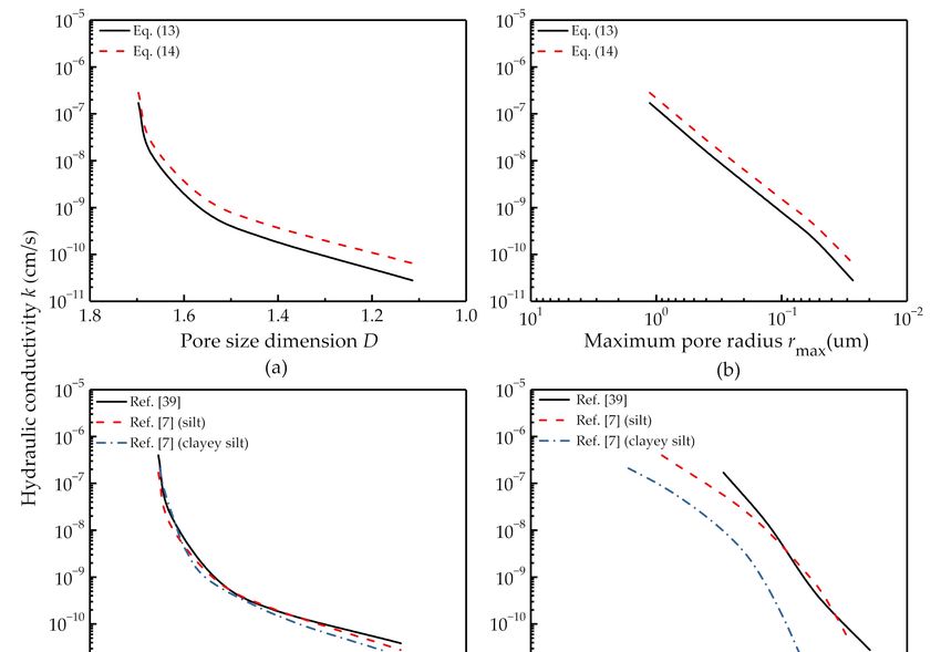
Water 2019, 11, 369                                                                                 4 of 20

Tarnawski [21] present their models to predict the hydraulic conductivity of frozen soil based on
different hydraulic conductivity models of melted soils, although this method tends to overestimate
hydraulic conductivity [3].
      Given the problems with the above methods, there is great need for a new approach to estimating
hydraulic conductivity. Since fractal theory (see Section 3) was first created, this method has been
applied to different areas to determine the permeability of porous material; for example, Yu [22,23]
proposed a fractal permeability model for fabrics and bi-dispersed porous media, predicting the
corresponding permeability well. Yao [24] investigated the fractal characteristics of coals using the
mercury porosimetry method, and analysed the influence of the fractal dimension of pores on the
permeability of coals. Pia [25] presented an intermingled fractal units model based on fractal theory
for the purpose of predicting the permeability of porous rocks. Xu [26] used fractal geometry to
describe soil pores and obtained the fractal dimension of pores from porosimetric measurements.
A permeability function was eventually put forward to predict the permeability of soils. The fractal
theory used by this study to estimate the permeability performed well for the chosen materials. The
pore size distribution of frozen soil was confirmed as satisfying the fractal characteristics [27–29]
required; therefore, we attempted to apply the fractal theory to determine its hydraulic conductivity.
      In the present study, a fractal model for hydraulic conductivity of saturated frozen soil was
presented. A method for determining the model parameters was also proposed. Model performance
was subsequently evaluated by comparing predictions with experimental data from the existing
literature and other models. Furthermore, the validity of Darcy’s law in saturated frozen soil
was explained.

3. Fractal Model for Hydraulic Conductivity of Frozen Soil

3.1. Fractal Theroy
     In classical Euclidean geometry, the dimensions of ordered objects are the integers; for example,
the dimensions of points, straight lines, planes, and volumes are 0, 1, 2 and 3, respectively. However,
for disordered objects such as irregular lines, planes or volumes, Euclidean geometry is not applicable.
To solve this problem, fractal geometry has been introduced. In fractal geometry, the dimension
of fractal objects is not an integer, but a fraction. Normally, 1 < D < 2 in two-dimensional
space and 2 < D < 3 in three-dimensional space. Fractal theory emerges based on fractal geometry.
Fractal theory describes and studies the objects from the perspective of fractal dimensions and its
mathematical methods. The fractal theory broke out of the traditional barriers of one-dimensional
lines, two-dimensional surfaces, three-dimensional spaces, bringing it closer to a description of the real
properties and states of complex systems, more consistent with the diversity and complexity of objects.

3.2. The Fractal Capillary Bundle Model of Frozen Soil
     The real size or geometric shape of pores are difficult to describe, meaning pores are sometimes
visualized as circular capillary tubes [30]. A capillary bundle model has consequently been proposed
and frequently applied [31–33]. Although the model is different from real soils, it contains many of
the same properties and so can be used to analyse the water flow in frozen soil [18]. As illustrated in
Figure 1, the pores are conceptualised as an assembly of tortuous capillary tubes.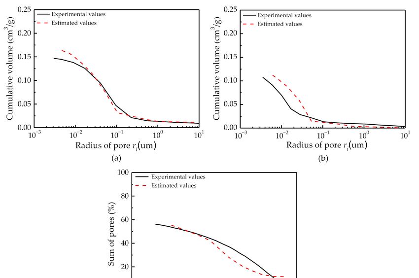
Water 2019,
Water 2019, 11,
11, 369
x FOR PEER REVIEW 55 of 21
of 20
Water 2019, 11, x FOR PEER REVIEW 5 of 21
Figure 1.
Figure Schematic of
1. Schematic of capillary
capillary bundle
bundle model
model of
of frozen
frozen soil.
soil.
Figure 1. Schematic of capillary bundle model of frozen soil.
To
To develop
develop the the fractal
fractal capillary
capillary bundle
bundle model,
model, we
we assumed
assumed the the frozen
frozen soil
soil was
was homogeneous
homogeneous
and To develop the fractal capillary bundle model, we assumed the frozen soil was homogeneous
and isotropic;
isotropic; thethe solid
solid matrix
matrix was
was incompressible;
incompressible; the the pores
pores could
could be be treated
treated as
as capillary
capillary tubes
tubes with
with
and isotropic;
different thethe
radii; solid matrix was
capillaries were incompressible;
initially filled the pores
with liquidcould
water beandtreated
the as capillary
water flow in tubes
the with
different
different radii; the capillaries were initially filled with liquid water and the water flow in the different
different
capillaryradii; theremain
capillaries were initially Thefilled with of
liquid water and the water flow in the different
capillary tubes
tubes remain independent;
independent; The freezing
freezing of pore
pore water
water started
started fromfrom macrospores
macrospores and and the
the
capillary
freezing tubes remain independent; The freezing of pore water started from macrospores and the
freezing temperature
temperature of of pore
pore water
water reduced
reduced with with the
the decrease
decrease of of pore
pore diameter. Figure 22 gives
diameter. Figure gives aa
freezing
schematictemperature
of the of pore water in reduced with the decrease of poresaturated
diameter.tubes
Figure
are2filled
gives a
schematic of the freezing
freezing process
process in capillary
capillary tubes,
tubes, where
where the
the fully
fully saturated tubes are filled with
with
schematic
liquid of the
water in freezing
the process
unfrozen in As
state. capillary
the tubes, where
temperature the fully
decreases, thesaturated
liquid tubesinare
water filled
larger withare
tubes
liquid water in the unfrozen state. As the temperature decreases, the liquid water in larger tubes are
liquid water inice
frozen the unfrozen state. As theremains.
temperature decreases,
ice the liquid water in larger tubes arethe
frozen into
into ice andand aa thin
thin liquid
liquid film
film remains. The The radii
radii of ice
of filled
filled tubes
tubes and
and the
the thickness
thickness of of the
frozen
liquidinto
film ice anddepend
both a thin onliquid film remains. The radii of ice filled tubes and the thickness of the
temperature.
liquid film both depend on temperature.
liquid film both depend on temperature.
Figure 2. Schematic of freezing process of capillary tubes.
Figure 2. Schematic of freezing process of capillary tubes.
Figure 2. Schematic of freezing process of capillary tubes.
3.3. Derivation of the Fractal Model to Determine the Hydraulic Conductivity of Frozen Soil
3.3. Derivation of the Fractal Model to Determine the Hydraulic Conductivity of Frozen Soil
3.3. Derivation of the Fractal
The cumulative poreModel to Determine
size distribution the Hydraulic
follows the fractal Conductivity
scaling lawof[34];
Frozen Soil the cumulative
therefore
numberThe cumulative pore
of pores satisfied: size distribution follows the fractal scaling law [34]; therefore the
The cumulative pore size distribution follows r the fractal
D
scaling law [34]; therefore the
cumulative number of pores satisfied: max
cumulative number of pores satisfied: N (≥ r ) = (4)
r D
armax D
where N is the cumulative number of pores r ) =rmax
N (≥ with
radius greater than or equal to r; rmax is (4) the
N (≥ r ) = r (4)
maximum radius (m) and, D is the pore size dimension, 1 < D < 2. Differentiating Equation (4) with
r
respect to r yields:
where N is the cumulative number of pores with a radius D −(greater greater than or equal to r ; r is the
where N is the cumulative number−ofdN pores
(≥ r )with
= Dr a max
radius r D+1) dr than or equal to r ; rmaxmaxis the(5)
maximum radius ( m ) and, D is the pore size dimension, 1 < D < 2 . Differentiating Equation (4)
maximum radius ( m ) and, D isnumber
the pore size dimension, 1 0,
with Equation
respect to(5)r gives the pore
yields: between the pore size and
with respect
which to r that
indicates yields:
pore number decreases with an increase in pore size.
D − ( D + 1)
−dN (≥ r ) = Drmax rD + 1) dr tubes with different radii; therefore, (5)
The soil pore system is assumed to
−dN (be
≥ ra) bundle
= Drmax Dof r −(capillary
dr (5)
the Hagen-Poiseuille equation can be used to describe the water flow in the soil, as given by [22,35]:
Equation (5) gives the pore number between the pore size r and r + dr . In Equation (5),
Equation (5) gives the pore number between the pore size r and r + dr . In Equation (5),
−dN > 0 , which indicates that pore number decreases g with
∆Hanan increase in pore size.
−dN > 0 , which indicates that pore number qdecreases r4
π ρwwith increase in pore size.
The soil pore system is assumed to be a=bundle of capillary
Le
8 ofη capillary tubes with different radii; therefore,(6)
The soil pore system is assumed to be a bundle tubes with different radii; therefore,
the Hagen-Poiseuille equation can be used to describe the water flow in the soil, as given by [22,35]:
the Hagen-Poiseuille equation can be used to describe the water flow in the soil, as given by [22,35]: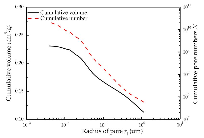
Water 2019, 11, 369                                                                                   6 of 20

where q is the water flow rate in a single capillary (m3 /s); r and Le are the radius and length of the
capillary, respectively (m); η is the dynamic viscosity of the fluid (Pa · s); ∆H is the hydraulic gradient;
ρw is the density of water (kg/m3 ); and g is gravitational acceleration (m/s2 ). The total flow rate Q
(m3 /s) can be obtained by integrating the single flow rate, q, from the minimum pore radius to the
maximum radius with the aid of Equation (6):
                                                              "            4− D #
                                           πρw g ∆H D
                            Z rmax
                                                                     r min
                      Q=−            qdN =              rmax 4 1 −                                       (7)
                             rmin           8η Le 4 − D              rmax

    Since 1 < D < 2, the exponent 4 − D > 2, rmin /rmax < 10−2 ; therefore, (rmin /rmax )4− D  1.
Then Equation (7) is reduced to:
                                      πρw g ∆H D
                                 Q=                   rmax 4                                   (8)
                                       8η Le 4 − D
     The average velocity Ja (m/s) through the capillaries can be obtained by dividing Q by the total
pore area Ap (m2 ):
                                          πρw g ∆H D
                                     Ja =                  rmax 4                                 (9)
                                          8η Ap Le 4 − D
      The total pore area in Equation (9) can be expressed as [36]:

                                                                πD (1 − ε)rmax 2
                                        Z rmax
                               Ap =              πr2 (−dN ) =                                          (10)
                                         rmin                       2−D

where ε is the porosity. Inserting Equation (10) into Equation (9) yields:

                                                  ρw g ∆H 2 − D rmax 2
                                          Ja =                                                         (11)
                                                   8η Le 4 − D 1 − ε

      The Darcy flux JT can be determined by using the Dupuit-Forchheimer equation:

                                                  ρw g ∆H ε 2 − D
                                     JT = εJa =                      rmax 2                            (12)
                                                   8η Le 1 − ε 4 − D

where τ is a tortuosity, which is the ratio between the length of soil column L (m) and the length of the
capillary Le (m). Comparing Equation (12) with Darcy’s law, JT = k ∆H     L , results in the expression for
the hydraulic conductivity as follows:

                                                 ρw g ε 2 − D
                                          k=                     rmax 2                                (13)
                                                 8ητ 1 − ε 4 − D

where k is the hydraulic conductivity. For a straight capillary bundle fractal model (τ         = 1), the
hydraulic conductivity is reduced to:

                                                 ρw g ε 2 − D
                                          k=                     rmax 2                                (14)
                                                  8η 1 − ε 4 − D

     It can be found from Equation (13) that for water flow through a given soil sample, the hydraulic
conductivity is related to the maximum pore size, pore size dimension, and tortuosity. Of these
parameters, maximum pore size plays a key role in affecting hydraulic conductivity. These parameters
reflect the pore structure characteristic of the soil, and each of them has a clear physical meaning,
which reveals a significant advantage of the model.
     In the model, ice is assumed to form first in the largest water-filled tubes upon freezing based on
the Gibbs-Thomson effect. The Gibbs-Thomson effect describes how a depression in the freezing point
is inversely proportional to pore size. Due to the free energy of the capillary wall, some water in the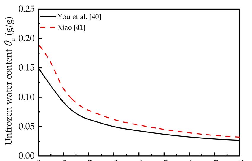
Water 2019, 11, 369                                                                                             7 of 20

vicinity of the capillary wall remains unfrozen at subzero temperatures; hence why the frozen capillary
is considered to be composed of an ice column and a thin liquid film in the vicinity of the tube wall.
As the solid phase is assumed to be incompressible, the radius of the capillary cannot be affected by
the frost heave of the water in the capillary. Therefore, the radius of the capillary is measured as the
sum of the radius of the ice column and the thickness of the thin liquid film. The radius of the ice
column can be assessed by the Gibbs-Thomson equation [37]:

                                                        2σsl     Tm
                                               ri i =                                                            (15)
                                                        Lf ·ρi Tm − T i

where, ri i (m) is the critical radius of ice column at T i (◦ C); σsl is the ice-liquid water interfacial
free energy, γ = 0.0818 J/m2 ; Lf is latent heat of fusion, L = 334.56 kJ/kg; ρi is the density of ice,
ρi = 917 kg/m3 ; and Tm is the freezing temperature of bulk water given in Kelvin, Tm = 273.15 K.
The thickness of the liquid water film can be assessed by [18]:
                                                                         1/3
                                           i     AH      Tm
                                          d = −                                                                  (16)
                                                6πρi L Tm − T i

where di is the film thickness of unfrozen water (m) and, AH is the Hamaker constant, AH = −10−19.5 J.
The soil freezing curve (SFC) describes how the volumetric content of unfrozen water decreases with a
decrease in the sub-zero temperature. The number of capillaries of radius ri can be determined using
the SFC. As shown in Figure 3, the SFC is divided into several different spaced water-content intervals
of width ∆θu i , according to the experimental points, and the temperature T θu i associated with the


decrease in θu i can be determined. All capillaries of radius r ≥ ri are assumed to be frozen when
T = T i . Thus, the number of capillaries N i frozen at T i , is equivalent to the increase in ice content
in real soil, ∆Vi i /πri i Le , where ∆Vi i is the increment of ice volume at T i . ∆Vi i can be calculated from
the SFC, then the cumulative number of capillaries N r ≥ ri is given by summing the number of


capillaries     i of
   Water 2019,N11,   radius
                   x FOR PEER ri REVIEW
                                 when r ≥ ri .                                                                8 of 21

          Figure 3. Scheme
            Figure          of of
                    3. Scheme  a physical approach
                                  a physical       to to
                                             approach determine thethe
                                                         determine  pore size
                                                                       pore   distribution
                                                                            size           of frozen
                                                                                 distribution        soil.
                                                                                              of frozen soil.

        The pore size dimension was determined by the accumulative pore size distribution. The
   cumulative pore size distribution of fractal capillaries follows the fractal power law; therefore, taking
   the logarithm of both sides of Equation (4) gives:
                                                                 lg N
                                                        D=                                                         (17)
                                                             lg ( rmax r )

        As seen in Equation (17), the pore size dimension was the slope of the accumulative pore size
   distribution in the double logarithmic coordinates, which was approximately a straight line. For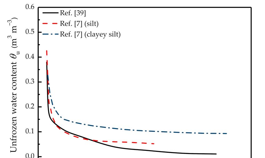
Water 2019, 11, 369                                                                               8 of 20

     The pore size dimension was determined by the accumulative pore size distribution.
The cumulative pore size distribution of fractal capillaries follows the fractal power law; therefore,
taking the logarithm of both sides of Equation (4) gives:

                                                    lgN
                                           D=                                                      (17)
                                                 lg(rmax /r )

      As seen in Equation (17), the pore size dimension was the slope of the accumulative pore size
distribution in the double logarithmic coordinates, which was approximately a straight line. For frozen
soil, the accumulative pore size distribution changed with temperature, leading to pore size dimension
changes with temperature. The pore size dimension of frozen soil at different subzero temperatures
needed to be determined using the accumulative pore size distribution at the corresponding
temperature, the calculation of which had already been described above. In Equation (13), the dynamic
viscosity of the water can be given as [18]
                                                       c
                                            η = η0 exp( )                                          (18)
                                                       T

where η0 = 9.62 × 10⁻⁷ Pa · s and c = 2046 K. Equation (18) yields µ = 10−3 Pa · s when T = 21.5 ◦ C.
The tortuosity can be assessed using the following relationship [34,35,38]

                                         τ = 1 + 0.41 ln(1/ε)                                      (19)

      In this model, the porosity is the ratio between the total unfrozen volume of capillaries and
the volume of the soil column. As the unfrozen capillaries are assumed to be completely filled with
unfrozen water, so the volume of unfrozen water can be conceived as the volume of the capillaries;
thus, the porosity is equivalent to the volumetric content of unfrozen water. To illustrate the fractal
Water 2019, 11,
hydraulic       x FOR PEER REVIEW
             conductivity   modeling process well, a flow diagram is given in Figure 4.          9 of 21

                            Figure 4.
                            Figure    Flow diagram
                                   4. Flow diagram of
                                                   of fractal
                                                      fractal model
                                                              model building.
                                                                    building.

4. Methods
      The present model was applied to existing literature on the measured hydraulic conductivity of
saturated frozen soil to test its validity. Some existing studies did measure saturated conductivity;
however, only a few simultaneously report the SFC, initial volumetric content and the dimension of
the soil column, which are required by the model. Thus, model testing was limited by the paucity of
the literature.
      Burt and Williams [7] and Tokoro et al. [39] measured saturated hydraulic conductivity using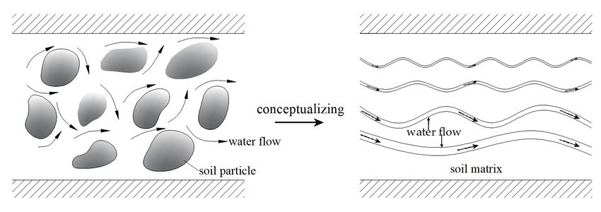
Water 2019, 11, 369                                                                                         9 of 20

4. Methods
      The present model was applied to existing literature on the measured hydraulic conductivity of
saturated frozen soil to test its validity. Some existing studies did measure saturated conductivity;
however, only a few simultaneously report the SFC, initial volumetric content and the dimension of
the soil column, which are required by the model. Thus, model testing was limited by the paucity of
the literature.
      Burt and Williams [7] and Tokoro et al. [39] measured saturated hydraulic conductivity using
self-developed experimental apparatus; their apparatus allows water to flow as a fluid. A summary of
the physical parameters of the soil samples is given in Table 1.

                                Table 1. Physical parameters of the soil samples.

        Soil Type       Length (cm)   Diameter (cm)     Dry Density (g/m3 )    Initial Water Content (m3 m−3 )
         Silt [7]           3              3.8                  1.52                        0.50
      clayey silt [7]       3              3.8                  3.8                         0.33
         Silt [39]          3               7                     7                         0.38

     Figure 5 presents the SFCs of the three soil samples. As shown, the freezing curve decreases
dramatically near 0 ◦ C, after which the freezing curve became gradual. This result was because the
proportion   ofx capillaries
Water 2019, 11,              with small radii increased as temperature decreased.
                 FOR PEER REVIEW                                                             10 of 21

                                         Figure 5. Soil
                                         Figure5.  Soil freezing
                                                         freezing curve.
                                                                   curve.

5. Results
5. Results
5.1. Cumulative Pore Size Distribution Curve
5.1. Cumulative Pore Size Distribution Curve
     Here, the experimental data from Tokoro et al. [39] were used as an example to describe the
      Here, the
calculation     experimental
             process           datathe
                     for finding     from  Tokoroconductivity
                                        hydraulic  et al. [39] were  used assoil.
                                                                 of frozen   an example
                                                                                   Figure 6topresents
                                                                                              describe the
                                                                                                        the
calculation  process  for finding   the  hydraulic conductivity   of  frozen soil. Figure  6 presents
cumulative pore size distribution estimated by the SFC, with the solid line representing the cumulative the
cumulative pore size distribution estimated by the SFC, with the solid line representing the
volume of pores and the dashed line representing the cumulative number of pores. The number of
cumulative volume of pores and the dashed line representing the cumulative number of pores. The
pores with small radii was markedly higher than the number with large radii. As the temperature
number    of pores with small radii was markedly higher than the number with large radii. As the
decreased, the maximum radius decreased which led to changes in the pore size distribution curve.
temperature    decreased, the maximum radius decreased which led to changes in the pore size
Additionally, the cumulative pore size distribution (the dashed line plotted in the double logarithmic
distribution curve. Additionally, the cumulative pore size distribution (the dashed line plotted in the
coordinates) is approximately a straight line, the slope of which was the pore size dimension.
double logarithmic coordinates) is approximately a straight line, the slope of which was the pore size
dimension.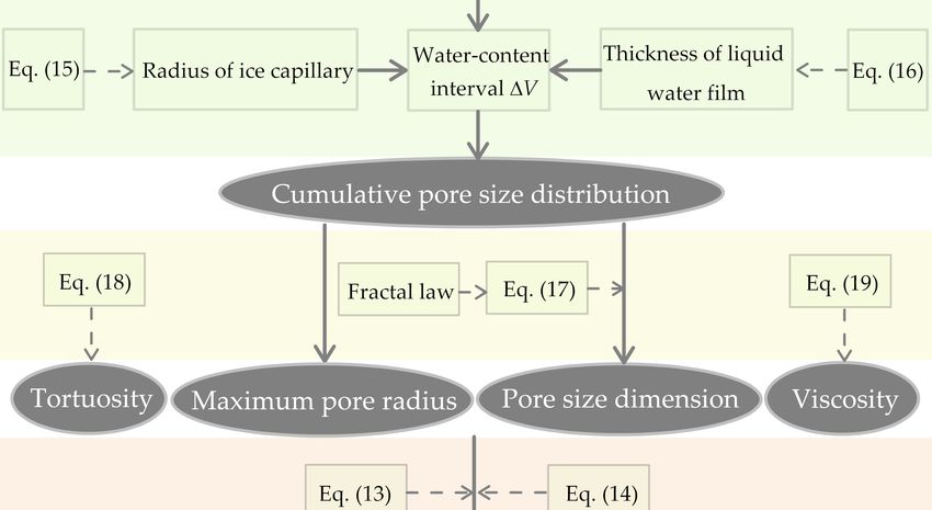
cumulative volume of pores and the dashed line representing the cumulative number of pores. The
number of pores with small radii was markedly higher than the number with large radii. As the
temperature decreased, the maximum radius decreased which led to changes in the pore size
distribution curve. Additionally, the cumulative pore size distribution (the dashed line plotted in the
double
Water logarithmic
2019, 11, 369 coordinates) is approximately a straight line, the slope of which was the pore size
10 of 20
dimension.
Figure 6. Pore size distribution determined by the soil freezing curve.
Figure 6. Pore size distribution determined by the soil freezing curve.
5.2. Maximum Pore Size, the Pore Size Dimension and Tortuosity
5.2. Maximum
Figure 7aPore Size,
shows thetherelationship
Pore Size Dimension
betweenand
theTortuosity
maximum pore radius and temperature, which
was calculated by Equations
Figure 7a shows (15) and (16).
the relationship The maximum
between the maximum porepore
radius decreased
radius with temperature.
and temperature, which
Figure 7b gives the
was calculated relationship
by Equations between
(15) the The
and (16). tortuosity
maximumand temperature, obtained using
pore radius decreased with Equation (19).
temperature.
The tortuosity
Figure 7b givesincreased with temperature.
the relationship between theFigure 7c presents
tortuosity the relationship
and temperature, between
obtained the Equation
using pore size
dimension and temperature,
(19). The tortuosity increased which was computed
with temperature. from7cthe
Figure cumulative
presents pore size distribution
the relationship between theusingpore
Water 2019,
Equation 11,
size dimension x FOR
(17). The PEER
andpore REVIEW
size dimension
temperature, whichdecreased linearlyfrom
was computed withthe
temperature.
cumulativeAs shown
pore size in 11 of 21
the figure,
distribution
the three
using parameters
Equation all pore
(17). The varied with
size temperature,
dimension which
decreased causedwith
linearly the temperature.
hydraulic conductivity
As shown in to the
be
figure, the three parameters all varied with temperature,
affected by the temperature according to Equation (13). which caused the hydraulic conductivity to
be affected by the temperature according to Equation (13).
Figure 7.
Figure 7. Variation
Variationof of
pore sizesize
pore dimension (a), maximum
dimension pore radius
(a), maximum (b) and(b)
pore radius tortuosity (c) with
and tortuosity
(c)‘with temperature.
temperature.
5.3.
5.3.Fractal
FractalValues
ValuesofofHydraulic
HydraulicConductivity
Conductivity
Figure
Figure8a
8apresents
presentsthe
thehydraulic
hydraulicconductivity
conductivitypredicted
predictedbybythethepresent
presentmodel
modelfor
fordifferent
differentpore
pore
size
sizedimensions
dimensionsfrom
fromEquations
Equations(13)
(13)and
and(14).
(14).Figure
Figure8b 8bshows
showsthethehydraulic
hydraulicconductivity
conductivitypredicted
predicted
by
bythe
thepresent
presentmodel
modelfor
fordifferent
differentmaximum
maximumpore poreradii
radiifrom
fromEquations
Equations(13)(13)and
and(14).
(14).The
Thehydraulic
hydraulic
conductivity
conductivity changed dramatically with the decrease in pore size dimension and maximumpore
changed dramatically with the decrease in pore size dimension and maximum pore
radius.
radius. This
This phenomenon
phenomenon can can be
be explained
explained as:
as: the
the decrease
decrease ofof pore
pore size
sizeand
andpore
poresize
sizedimension
dimension
causing a decrease in the number of capillaries, as well as the increase in the tortuosity causing an
increase in water flow paths, leading to a decrease in flow rate. Of all these influencing factors, pore
size plays a role in affecting hydraulic conductivity.
In the same way, the hydraulic conductivities of the three soil samples were predicted by the
present model for different temperature and volumetric water content from Equation (13). The resultsWater 2019, 11, 369 11 of 20
causing a decrease in the number of capillaries, as well as the increase in the tortuosity causing an
increase in water flow paths, leading to a decrease in flow rate. Of all these influencing factors, pore
size plays a role in affecting hydraulic conductivity.
In the same way, the hydraulic conductivities of the three soil samples were predicted by
the present model for different temperature and volumetric water content from Equation (13).
The results are shown in Figure 8c,d. From Figure 8c, the hydraulic conductivity changed dramatically
within −1 ◦ C, with similar results observed by Burt et al. [7] and Miller et al. [8]. These results can be
explained by the fact that the decrease in temperature caused a decrease of the pore size and pore size
dimension and increase of the tortuosity as shown in Figure 7, leading to a decrease in the hydraulic
conductivity. Figure 8d shows the relationship between the hydraulic conductivity and volumetric
water content,
Water 2019, calculated
11, x FOR from Equation (13). Figure 8d shows that the hydraulic conductivity increases
PEER REVIEW 12 of 21
with an increased in unfrozen water content.
Figure 8. The effect of pore size dimension (a), maximum pore radius (b), temperature (c) and unfrozen
Figure 8. The effect of pore size dimension (a), maximum pore radius (b), temperature (c) and
water content (d) on hydraulic conductivity.
unfrozen water content (d) on hydraulic conductivity.
6. Discussion
6. Discussion
6.1. Model Application
6.1. Model
FigureApplication
9 presents the comparison between the fractal model and the experimental data, with the
symbols representing
Figure 9 presents the comparison
experimental data, and
between thethe dashed
fractal lineand
model and dashed-dot
the experimental linedata,
representing
with the
the predictions
symbols by the the
representing present models calculated
experimental data, andfrom Equations
the dashed line(13)
andand (14), respectively.
dashed-dot In both
line representing
cases, the present
the predictions bymodel was inmodels
the present close agreement
calculated with
fromthe experimental
Equations data.
(13) and (14),From Figure 9a,Inusing
respectively. both
Equation (13), the present model shows good agreement with the experimental data
cases, the present model was in close agreement with the experimental data. From Figure 9a, using except for the
data point(13),
at 0.25 ◦ C; however,
Equation the present modelusing Equation
shows (14), the present
good agreement with themodel overrateddata
experimental the except
experimental
for the
data. Figureat9b
data point shows
0.25 that usingusing
°C; however, Equation (14), the
Equation present
(14), modelmodel
the present showed good agreement
overrated with the
the experimental
experimental
data. Figure 9b data while
shows using
that Equation
using (13),
Equation thethe
(14), present model
present modelunderestimate
showed good theagreement
experimental
withdata.
the
Figure 9c indicates
experimental the present
data while using model showed
Equation a slight
(13), the difference
present from the experimental
model underestimate data; however,
the experimental data.
Figure 9c indicates the present model showed a slight difference from the experimental data;
however, the behavior of the experimental data is approximately captured by the present model.
Overall, the present model based on fractal theory showed close agreement with the experimental
data. Thus, the validity of the present model was verified.Water 2019, 11, 369 12 of 20
the behavior of the experimental data is approximately captured by the present model. Overall, the
present model based on fractal theory showed close agreement with the experimental data. Thus, the
validity of11,
Water 2019, the present
x FOR PEERmodel
REVIEWwas verified. 13 of 21
Figure9.9. Comparison
Figure Comparison of of the
the model
model results
resultsand
and experimental
experimental data.
data. (a)
(a) Tokoro
Tokoroet
etal.
al.[39]
[39](silt);
(silt);(b)
(b)Burt
Burt
and Williams [7] (silt); (c) Burt and Williams [7] (clayey silt).
and Williams [7] (silt); (c) Burt and Williams [7] (clayey silt).
The
Thedifferences
differences between the predictions
between and experimental
the predictions data can data
and experimental be translated
can be into quantifiable
translated into
terms by means
quantifiable of the
terms bymean squared
means of the error,
meanMSE, which
squared is anMSE,
error, indicator
whichofisthe
anoverall magnitude
indicator of the
of the overall
residuals.
magnitude The MSEresiduals.
of the is computed
The as follows
MSE is computed as follows
N 2 2
11 N ln( k ) − ln( k )
MSE == ∑
MSE
N
N i =1 e , i ) − ln( k
ln(k e,i i
p ,p,i ) (20)
(20)
i =1
is the
where NNis the number ofofexperimental
experimentaldata points;k ke ,is
datapoints; is the ith measured hydraulic conductivity
where number e,i i the ith measured hydraulic conductivity
(m/s) ) and
( m / sand k p,ikis is the ith predicted hydraulic conductivity ( m /Table
p , i the ith predicted hydraulic conductivity (m/s). s ). Table 2 summarises
2 summarises the MSE
the MSE for
for the
three data sets. As shown, the present model–using Equations (13) and (14)—made
the three data sets. As shown, the present model–using Equations (13) and (14)—made the best the best prediction
for the Tokoro’s
prediction for the [39] silt data[39]
Tokoro’s set silt
anddata
Burtset
and Williams’
and Burt and [7]Williams’
silt data set, respectively.
[7] silt data set, respectively.
Table2.2.Model
Table Modelprediction
predictionstatistics
statisticsfor
forvarious
variousdata
datasets.
sets.
Squared Error
Reference
Present Mean Mean
Squared Squared Error
Model Error −0.25 ◦ C −0.3 ◦ C −0.35 ◦ C −0.4 ◦ C −0.45 ◦ C
Reference Present Model Squared
Equation (13) 0.34 1.62 °C
−0.25 0.08 °C
−0.3 0
−0.35 °C 0.001
−0.4 °C 0.01
−0.45 °C
Tokoro et al. [39] Error
Equation (14) 0.41 0.55 0.08 0.33 0.54 0.55
Burt and Williams Equation (13) 0.91 2.23 1.02 0.55 0.30 0.47
Tokoro et[7]al.
(silt) Equation (13)
Equation (14) 0.34
0.21 1.62
0.84 0.08
0.21 0.02 0 0 0.001 0 0.01
Burt[39]
and Williams Equation (13) 0.98 3.50 1.19 0 0.22 0
(clayey silt) [7] Equation (14)
Equation (14) 0.41
0.78 0.55
1.98 0.08
0.41 0.33
0.16 0.970.54 0.40 0.55
Burt and Equation (13) 0.91 2.23 1.02 0.55 0.30 0.47
Williams (silt)
[7] Equation (14) 0.21 0.84 0.21 0.02 0 0
Burt and Equation (13) 0.98 3.50 1.19 0 0.22 0
Williams
(clayey silt) [7] Equation (14) 0.78 1.98 0.41 0.16 0.97 0.40Water 2019, 11,
Water 2019, 11, 369
x FOR PEER REVIEW 13 of
14 of 20
21
As an additional test, the present fractal model was further compared with past models. The
As an additional test, the present fractal model was further compared with past models.
following three models were considered: the Nixon model [13], Mao et al. model [16] and Jame and
The following three models were considered: the Nixon model [13], Mao et al. model [16] and
Norum model [14]. Here, the experimental data from the study by Tokoro [39] were used as an
Jame and Norum model [14]. Here, the experimental data from the study by Tokoro [39] were used
example. In the Nixon model, k0 and δ were obtained using the kf − T relationship in a log-log
as an example. In the Nixon model, k0 and δ were obtained using the kf − T relationship in a log-log
coordinate. The
coordinate. The value of k0k0and
value of and δ were
δ were 2.0 ×2.010 10−10
×−10 cm/sand
cm/s − 2.273,
and−2.273, respectively.
respectively. In In
thethe
MaoMao et
et al.
model and and
al. model the Jame and Norum
the Jame model,model,
and Norum the value ku was
theofvalue of8.1ku ×was 10−83.1×× θ10 6.21
u −3 × cm/s and θiand
θu 6.21 cm/s values
θi
were calculated from the SFC, θi = θw ρw /ρi . In the Jame and Norum model, the impedance factor
values were calculated from the SFC, θi = θw ρw ρi . In the Jame and Norum model, the impedance
was determined by the empirical constant E. To avoid an arbitrary choice of impedance factor, the
factor wasconstant
empirical determined E wasbydetermined
the empirical constant
using the methodE . Toproposed
avoid anby arbitrary
Shang et choice of impedance
al. [17]. The experimentalfactor,
the empirical ◦constant ◦ E was determined
◦ using the method proposed
data at −0.25 C, −0.3 C and −0.35 C were used to determine the empirical constants, respectively.by Shang et al. [17]. The
experimental
The data at
corresponding −0.25 °C,constants
empirical −0.3 °C andE were−0.35 °C were
−0.48, −2.82used
andto−determine the empirical constants,
3.66, respectively.
The corresponding empirical constants E
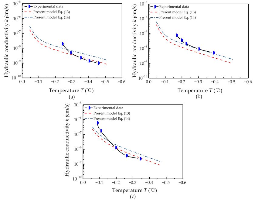
Figure 10 presents a visual comparison of various models for the silt data−3.66,
respectively. were −0.48, −2.82 and set fromrespectively.
Tokoro [39].
Figure 10 presents a visual comparison of various models for the silt
The inferences on model performance can be drawn from model predictions for the experimental data set from Tokoro [39].
The inferences
data. As shown, onthemodel
Nixon performance can bethe
model predicted drawn from model
experimental datapredictions
reasonably.forThis the isexperimental
ascribed to
data. As shown, the Nixon model predicted the experimental data
the fact that the model was determined from experimental data. Generally, the Mao reasonably. This is ascribed to the
et al. model
fact that the
overrated the model was determined
experimental data. For the fromJame experimental
and Norum data. Generally,
model, when Ethe = Mao
−0.48; et the
al. model
model
deviated greatly from the experimental data; however, a significant improvement was observedmodel
overrated the experimental data. For the Jame and Norum model, when E = −0.48 ; the when
deviated
E = −2.82greatly
and E = from the Itexperimental
−3.66. was found that data;thehowever,
Jame and aNorumsignificant
model improvement was observed
changed dramatically with
when E = −2.82 and E = −3.66 . It was found that the Jame and Norum model
the impedance factor. This shortcoming leads to a difficulty in accurately predicting the experimental changed dramatically
with Using
data. the impedance
Equation (13)factor. This
in the shortcoming
present model showed leads much
to a difficulty in accurately
closer agreement with thepredicting
experimental the
experimental data. Using Equation (13) in the present model showed much closer
data. Moreover, the present model using Equation (13) is close to the Nixon model. Using Equation (13) agreement with
thethe
in experimental
present model data. Moreover,
with Equationthe (13)present
overrated modelthe using Equation
experimental (13)
data is closethis
overall; to may
the Nixon model.
be attributed
Using Equation (13) in the present model with Equation
to the fact that the water flow path in the soil was tortuous. (13) overrated the experimental data overall;
this may be attributed to the fact that the water flow path in the soil was tortuous.
Figure 10. Comparison of the experimental data with different models for Tokoro [39] silt.
Figure 10. Comparison of the experimental data with different models for Tokoro [39] silt.
Table 3 summarises the MSE for the various models used to evaluate the model performance.
Table 3 summarises the MSE for the various models used to evaluate the model performance.
As shown, the MSE value for the Nixon model is lowest, at 0.33, followed by the present model with
As shown, the MSE value for the Nixon model is lowest, at 0.33, followed by the present model with
Equation (13) where the MSE was 0.34. In contrast, the present model with Equation (13) is close
Equation (13) where the MSE was 0.34. In contrast, the present model with Equation (13) is close to
to the Nixon model, which was determined by the experimental data. Using Equation (13) in the
the Nixon model, which was determined by the experimental data. Using Equation (13) in the present
present model, the squared error at −0.25 ◦ C was much higher than that at the other temperatures.
model, the squared error at −0.25 °C was much higher than that at the other temperatures. This
This difference can be attributed to experimental error and model error. The latter error may be related
difference can be attributed to experimental error and model error. The latter error may be related to
to the cracks caused by frost heave. Cracks are preferential flow paths, which result in an increase in
the cracks caused by frost heave. Cracks are preferential flow paths, which result in an increase in
conductivities. This influence of frost heave on the pore structure was not considered in the fractal
conductivities. This influence of frost heave on the pore structure was not considered in the fractal
model; however, on the whole, the difference was small. The MSE value for the Mao et al. model
model; however, on the whole, the difference was small. The MSE value for the Mao et al. model and
Jame and Norum model ( E = −0.48 ) was approximately 4 and 9 times larger, respectively, than forWater 2019, 11, 369 14 of 20
and Jame and Norum model (E = −0.48) was approximately 4 and 9 times larger, respectively, than
for the present model with Equation (13). The MSE for the Jame and Norum model (E = −2.82 and
E = −3.66) was close to that of the present model using Equation (14).
Table 3. Comparison results between various models.
Mean Squared Squared Error
Model Type
Error −0.25 ◦ C −0.3 ◦ C −0.35 ◦ C −0.4 ◦ C −0.45 ◦ C
Present model Equation (13) 0.34 1.62 0.08 0.001 0.009 0.01
Present model Equation (14) 0.41 0.55 0.08 0.33 0.54 0.55
Nixon model [13] 0.33 1.45 0.05 0.01 0.06 0.06
Mao et al. model [16] 1.37 0.03 0.80 1.55 2.14 2.32
Jame and Norum model [14]
2.96 0.14 2.19 3.47 4.36 4.66
E = −0.48
Jame and Norum model [14]
0.40 0.84 0.02 0.22 0.46 0.48
E = −2.82
Jame and Norum model [14]
0.39 1.75 0.12 0.0007 0.03 0.04
E = −3.66
In contrast, the fractal model provided a good agreement with the hydraulic conductivity data
overall. Moreover, comparison with other models revealed the following advantages of the fractal
model: fewer parameters; parameters are easy to obtain; each of the parameters has a clear physical
meaning; and no measured conductivity is required in the model. Additionally, the fractal model can
explain the reason for hydraulic conductivity changing with temperature; however, the influence of
frost heave on the pore structure of frozen soil is not considered in the model, which may result in
underestimating of the experimental data.
The present model has some limitations. Firstly, the model may be not valid in sandy soils, as
these contain massive large pores that will freeze once temperature is lower than zero degrees Celsius,
according to the SFC and Gibbs-Thomson equation. Second, the model does not consider the influence
of the difference in SFC determined by the different methods on the hydraulic conductivity of saturated
frozen soil. We expect this effect would not be pronounced when estimating the hydraulic conductivity,
as hydraulic conductivity largely depends on pore radius. Third, the model does not consider the
influence of frost heave on the pore structure of frozen soil, which may result in underestimating the
experimental data. We expect this effect to be less pronounced in high-temperature frozen soil, where
only slight frost heave occurs. Fourth, the model does not consider the influence of closed pores on
hydraulic conductivity, which will result in overrating the hydraulic conductivity. Lastly, the model is
only valid for soils fulfilling the fractal laws.
6.2. Comparison of the Cumulative Pore Size Distribution Determined by the SFC and Mercury Intrusion
Porosimetry (MIP)
The SFC was used to determine pore size distribution in the present study. To verify this method,
MIP was compared with this method. You et al. [40] and Xiao [41] measured the pore size distribution
of silty clay using MIP. Figure 11 represents the SFC of the two soil samples. The solid line represents
the freezing curve of You et al. [40], and the dashed line represent that of Xiao [41].Water 2019, 11, x FOR PEER REVIEW 16 of 21
Water 2019,11,
Water2019, 11,369
x FOR PEER REVIEW 15 of
16 of 20
21
Figure 11. Soil freezing curves of the soils.
Figure 11. Soil freezing curves of the soils.
Figure 11. Soil freezing curves of the soils.
Figure 12
Figure 12 shows
shows the
the comparison
comparisonofofpore poresize
sizedistribution
distribution determined
determined by bythethe
SFCSFC andandMIP.MIP.
The
solid lines
Figure represent
12 shows the
the pore size
comparison distribution
of pore determined
size distributionby MIP and
determined the
The solid lines represent the pore size distribution determined by MIP and the dashed lines representdashed
by the lines
SFC represent
and MIP. the
The
pore
solid
the poresize
lines distributions
represent
size determined
the pore
distributions bybythe
thesoil
size distribution
determined soilfreezing
determined
freezingby curve.
MIP It
curve. Itcan
and thebe
can seen
dashed
be that the
linesthe
seen that pore size
represent
pore size
the
distribution
pore size determined
distributions by the
determined SFC bycaptured
the soil the distinctive
freezing curve.feature
It can
distribution determined by the SFC captured the distinctive feature of the pore size distributionofbethe pore
seen thatsizethedistribution
pore size
determinedby
distribution
determined by MIPwell;
well;however,
determined
MIP however,
by the SFC this methodthe
captured
this method overrated
distinctive
overrated thesmaller
the smaller
featureporespores measured
of themeasured
pore sizeby by MIP.This
This
distribution
MIP.
resultcould
couldbe
determined
result beascribed
by ascribed
MIP well;toto thefact
however,
the factthat
thatthe
this theisolated
isolated
method pores—those
overrated the smaller
pores—those thatpores
that hadno
had no communication
measured
communication with
by MIP.with
This
the exterior
result could of
bethe sample
ascribed tocould
the not
fact be measured
that the isolatedby MIP in any
pores—those event,
thatregardless
the exterior of the sample could not be measured by MIP in any event, regardless of the pressure had no of the pressure
communication used
with
[42],exterior
the
used However,
[42], However,the
of the isolated
sample
the could
isolated pores
not could
poresbecouldbebe
measuredfilledbywith
filled withwater,
MIP inwater, which
any event, isis considered
whichregardless
considered of thein the pore
poreused
inpressure
the size
size
distribution
[42], However,
distribution determined
determined bybythe
the isolated the SFC.
pores
SFC. Fagerlund
could be filled
Fagerlund [37]
[37]withused
used aasimilar
water, similar
which method totoaccurately
is considered
method accurately
in the predict the
pore the
predict size
pore size
distribution distribution
determined in the
by range
the SFC.0.02 µm~0.5
Fagerlund µm
[37] for a
used certain
a sand-lime
similar method brick
to
pore size distribution in the range 0.02 µm~0.5 µm for a certain sand-lime brick as shown in Figure 12c. as shown
accurately in Figure
predict the
12c. size distribution in the range 0.02 µm~0.5 µm for a certain sand-lime brick as shown in Figure
pore
12c.
Figure12.
Figure 12. Comparison
Comparison of the the pore
poresize
sizedistribution
distributiondetermined
determinedbybySFC and
SFC byby
and MIP. (a)(a)
MIP. Xiao [41];
Xiao (b)
[41];
You
(b) et et
You
Figure al.al.
12. [40]; (c)(c)
[40];
ComparisonFagerlund
of the[42].
Fagerlund [42].size distribution determined by SFC and by MIP. (a) Xiao [41]; (b)
pore
You et al. [40]; (c) Fagerlund [42].Water 2019, 11, x FOR PEER REVIEW 17 of 21
6.3. Vvalidity of Darcy’s Law
Water 2019, 11, 369 16 of 20
The present model was determined by Darcy’s law. Although Darcy’s law is widely applied to
frozen soil, the validity of Darcy’s law in frozen soil remains controversial. Several previous studies
have
6.3. shown of
Vvalidity that Darcy’s
Darcy’s Lawlaw is applicable in frozen soil, at least in high-temperature frozen soil; for
example, Burt and William [7] found a linear relationship between the hydraulic gradient and
The present
discharge model
for clayey silt was
withindetermined by Darcy’s
−0.5 °C using a laboratorylaw. Although
experiment. Darcy’s law isand
Horiguchi widely applied
Miller to
[8] found
frozen soil, the validity of Darcy’s law in frozen soil remains controversial. Several
the flux linearly changed with hydraulic conductivity for silt at different temperature within −0.15 previous studies
have shown[39]
°C. Tokoro thatobserved
Darcy’s thelawsame
is applicable in frozen
experimental soil, at least
phenomenon in within
for silt high-temperature
−0.5 °C. frozen soil;
for example, Burt and William [7] found a linear relationship between the
To further account for the validity of Darcy’s law, a theoretical proof based on the capillaryhydraulic gradient and
discharge for clayey silt within −0.5 ◦ C using a laboratory experiment. Horiguchi and Miller [8] found
bundle model and Reynolds number was proposed. The Reynolds number Re is always used◦ to
the flux linearly changed with hydraulic conductivity for silt at different temperature within −0.15 C.
justify the
Tokoro [39]flow state of
observed thethe
samefluid in the capillaries
experimental phenomenon for silt within −0.5 ◦ C.
To further account for the validity of Darcy’s law, 2rcraρv
theoretical proof based on the capillary bundle
model and Reynolds number was proposed. The R e
= Reynolds number Re is always used to justify(21) the
μ
flow state of the fluid in the capillaries
where rcr is the critical pore radius ( m ); ρReis=the 2rdensity
cr ρv of the fluid ( kg / m 3 ); and v is the flow
(21)
µ
velocity ( m / s ). The flow velocity can be obtained by dividing water flow rate by the cross area of a
3
single rcapillary
where cr is the critical pore radius (m); ρ is the density of the fluid (kg/m ); and v is the flow velocity
(m/s). The flow velocity can be obtained by dividing 2
water flow rate by the cross area of a single
r ρ g ΔH
capillary v= q πr = 2 w
(22)
2
8 η
r ρw g ∆H
2 Le
v = q/πr = (22)
8 η Le
Substituting Equation (22) into Equation (21), the critical pore radius rmax for laminar flow was
Substituting Equation (22) into Equation (21), the critical pore radius rmax for laminar flow was
obtained as
obtained as s
3 44RR eμµ22ττ
rmax== 3 ρ e22 gi
rmax (23)
(23)
w
ρ w gi
The unfrozen water film is much smaller than the radius of capillaries; therefore, the geometry of
The unfrozen water film is much smaller than the radius of capillaries; therefore, the geometry
ice in frozen soil is assumed to be identical to that of air in drying soil. Thus, the relationship between
of ice in frozen soil is assumed to be identical to that of air in drying soil. Thus, the relationship
the matric potential of frozen soil and temperature can be estimated using the generalised form of the
between the matric potential of frozen soil and temperature can be estimated using the generalised
Clausius-Clapeyron equation, treating ice pressure the same as gauge pressure
form of the Clausius-Clapeyron equation, treating ice pressure the same as gauge pressure
Lf Tm − ∆T
h= L fln
T − ΔT (24)
h =g ln mTm (24)
g Tm
where |h| is the hydraulic head (m) and ∆T is the freezing temperature depression (◦ C). Figure 13
where | h| is the hydraulic head ( m ) and ΔT is the freezing temperature depression (°C). Figure
presents the |h|−∆T relationship obtained using Equation (24).
13 presents the | h | −ΔT relationship obtained using Equation (24).
Figure 13. Relationship between the hydraulic head and temperature for frozen soil estimated using
Figure 13. Relationship between the hydraulic head and temperature for frozen soil estimated using
the Clausius-Clapeyron equation.
the Clausius-Clapeyron equation.You can also read