D3.1 Flight flexibility and in the ADAPT hotspots solution
←
→
Page content transcription
If your browser does not render page correctly, please read the page content below
EXPLORATORY RESEARCH

D3.1 Flight flexibility and
hotspots in the ADAPT
solution
Deliverable 3.1
ADAPT
Grant: 783264
Call: H2020-SESAR-2016-2
 SESAR-ER3-03-2016 Optimised ATM Network
Topic:
 Services: TBO
Consortium coordinator: Università degli Studi di Trieste
Edition date: 28 February 2019
Edition: 01.01.00
EDITION 01.01.00

Authoring & Approval

Authors of the document
Name/Beneficiary Position/Title Date
Tatjana Bolic/ Università degli Studi WP 3 Leader / Senior researcher 25 February 2019
di Trieste
Lorenzo Castelli/ Università degli Project Coordinator / Assistant professor 25 February 2019
Studi di Trieste
Eric Medvet/ Università degli Studi Team member / Assistant professor 25 February 2019
di Trieste
Thomas Parisini/ Università degli Team member / Full professor 25 February 2019
Studi di Trieste
Giovanni Scaini/ Università degli Team member / Researcher 25 February 2019
Studi di Trieste

Reviewers internal to the project
Name/Beneficiary Position/Title Date
Mihaela Mitici /TU Delft WP 4 Leader/Assistant professor 26 February 2019

Approved for submission to the SJU By — Representatives of beneficiaries involved in the project
Name/Beneficiary Position/Title Date
Lorenzo Castelli/ Università degli Project Coordinator / Assistant Professor 28 February 2019
Studi di Trieste

Rejected By - Representatives of beneficiaries involved in the project
Name/Beneficiary Position/Title Date

Document History
Edition Date Status Author Justification
01.00.00 21 December 2018 Release ADAPT Consortium New document for review
 by SJU
01.01.00 28 February 2019 Release ADAPT Consortium Review comments
 addressed

2 © – 2019 – Università degli Studi di Trieste, Technische Universiteit
 Delft, University of Westminster, Deep Blue, Università degli Studi di
 Palermo. All rights reserved. Licensed to the SESAR Joint Undertaking
 under conditions.
D3.1 FLIGHT FLEXIBILITY AND HOTSPOTS IN THE ADAPT SOLUTION

ADAPT
ADVANCED PREDICTION MODELS FOR FLEXIBLE TRAJECTORY BASED
OPERATIONS
This deliverable is part of a project that has received funding from the SESAR Joint Undertaking under
grant agreement No 783264 under European Union’s Horizon 2020 research and innovation
programme.

Abstract
This deliverable reports the formulation and implementation of a deterministic model (European
Strategic Flight Planning (ESFP) model) to define flight trajectories and associated time windows at the
strategic level.

The EFPS model assigns the trajectory, departure time and flexibility measure for all the flights in the
data instance (the ECAC network for the entire day of traffic). Apart from that, for each constrained
flight the limiting sector-hour is identified, which can be of help in case the airline user would prefer
to re-route the flight in order to increase its flexibility.
Furthermore, the model gives the list of saturated sector-hours throughout the day. Keep in mind that
the configurations are changed during the day. Having the information on the saturated sectors, and
their criticality index, the ANSPs could take mitigation actions in order to improve the situation. For
example, a supervisor having one or two saturated sectors, both with the low criticality index, might
decide that the current configuration is good enough as even if the capacity ends up being violated it
will be for a small number of flights, which in many cases is what already happens in every-day
operations. However, if there are few sector-hours within an ACC that have high criticality indexes, the
supervisor might decide to change the configuration into a one that brings more capacity.

 3
 © – 2019 – Università degli Studi di Trieste, Technische Universiteit Delft,
 University of Westminster, Deep Blue, Università degli Studi di Palermo.
 All rights reserved. Licensed to the SESAR Joint Undertaking under conditions.
EDITION 01.01.00

Table of Contents

EXECUTIVE SUMMARY ................................................................................................................................ 6
1 INTRODUCTION .................................................................................................................................. 8
 1.1 INTRODUCING TIME WINDOWS (TW) ............................................................................................................. 9
 1.2 INTRODUCING CAPACITY MATTERS ................................................................................................................. 10
2 EFPS MODEL..................................................................................................................................... 13
 2.1 SATA - STRATEGIC AIR TRAFFIC ASSIGNMENT ................................................................................................. 13
 2.1.1 Notation for SATA model .................................................................................................................. 14
 2.1.2 Decision variables ............................................................................................................................. 15
 2.1.3 Objective functions ........................................................................................................................... 15
 2.1.4 Constraints ........................................................................................................................................ 17
 2.2 TIME WINDOWS MODEL ............................................................................................................................. 18
 2.2.1 Notation ............................................................................................................................................ 18
 2.2.2 Decision variables ............................................................................................................................. 19
 2.2.3 Objective function ............................................................................................................................. 19
 2.2.4 Constraints ........................................................................................................................................ 19
 2.3 VARIANTS OF TW MODEL ............................................................................................................................ 22
 2.3.1 Conservative TW model .................................................................................................................... 22
 2.3.2 Proportional TW model .................................................................................................................... 22
 2.3.3 Intermediate TW model .................................................................................................................... 23
3 DATA INSTANCE ............................................................................................................................... 25
 3.1 FLIGHTS.................................................................................................................................................... 25
 3.2 AIRSPACE CONFIGURATION AND CAPACITIES OF RESOURCES................................................................................ 25
 3.3 AIRCRAFT TYPES AND RELATED FLIGHT COSTS ................................................................................................... 25
 3.4 AIRLINE TYPES AND COST PROFILES ................................................................................................................ 26
 3.5 ROUTES AND DEPARTURE TIMES .................................................................................................................... 26
 3.6 ROUTE CHARGES AND UNIT RATES ................................................................................................................. 26
4 COMPUTATIONAL EXPERIMENTS ...................................................................................................... 27
 4.1 RESULTS ................................................................................................................................................... 27
 4.1.1 TW duration ...................................................................................................................................... 28
 4.1.2 Constrained flights and saturated sector-hours ............................................................................... 31
 4.2 FEASIBILITY ............................................................................................................................................... 33
 4.3 SENSITIVITY ............................................................................................................................................... 35
5 CONCLUSIONS AND NEXT STEPS........................................................................................................ 38
 5.1 DISCUSSION .............................................................................................................................................. 38
 5.2 NEXT STEPS ............................................................................................................................................... 39
6 ACRONYMS ...................................................................................................................................... 40
7 REFERENCES ..................................................................................................................................... 41
APPENDIX A TURNAROUND CONSTRAINTS ........................................................................................... 42

4 © – 2019 – Università degli Studi di Trieste, Technische Universiteit
 Delft, University of Westminster, Deep Blue, Università degli Studi di
 Palermo. All rights reserved. Licensed to the SESAR Joint Undertaking
 under conditions.
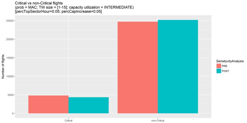
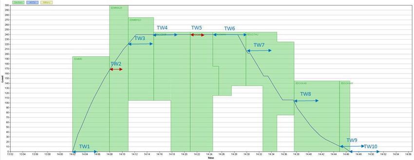
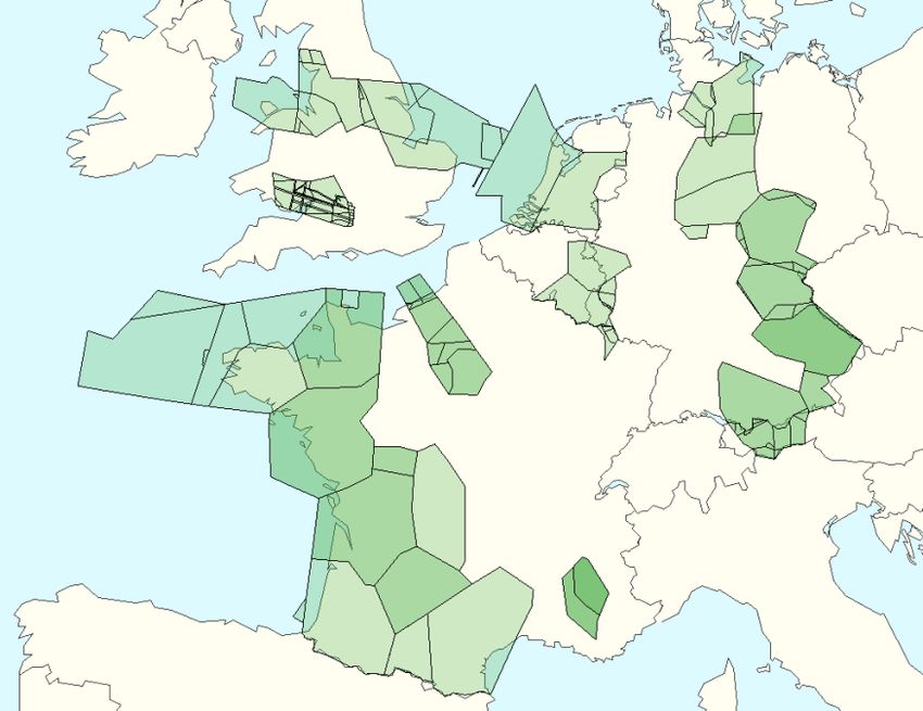
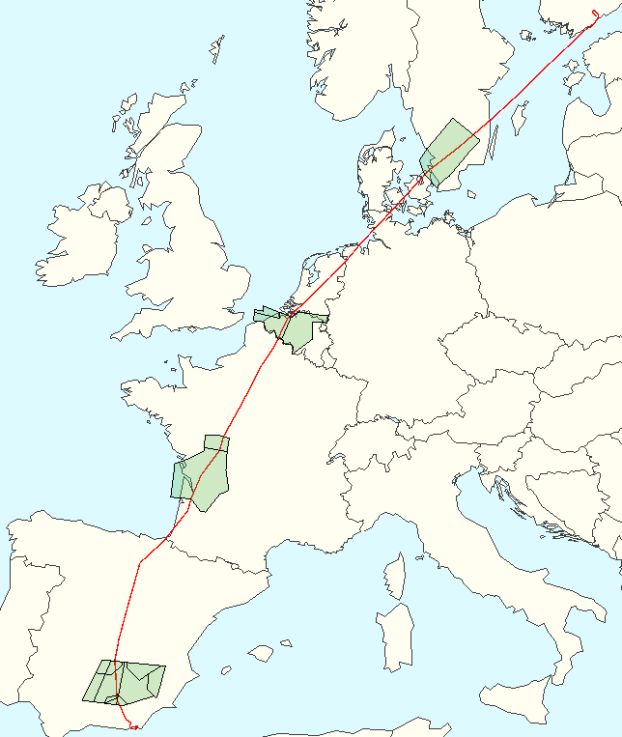
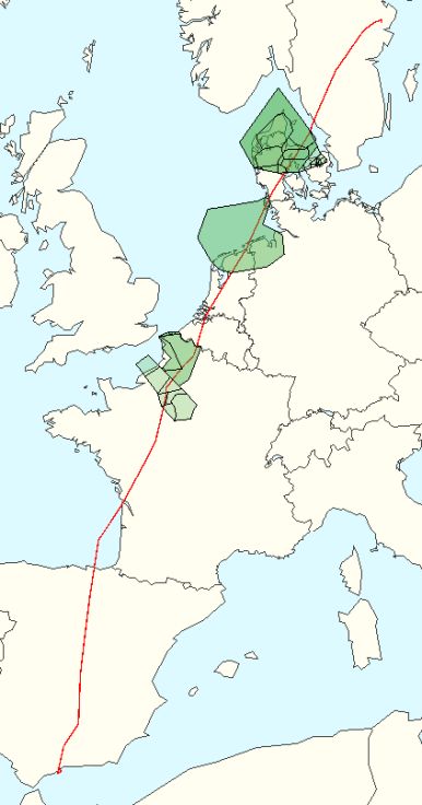
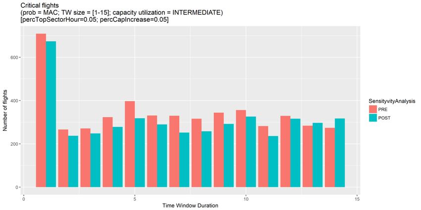
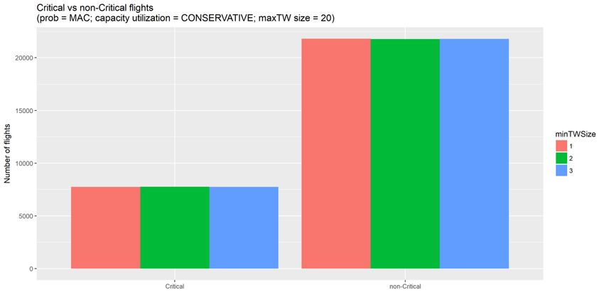
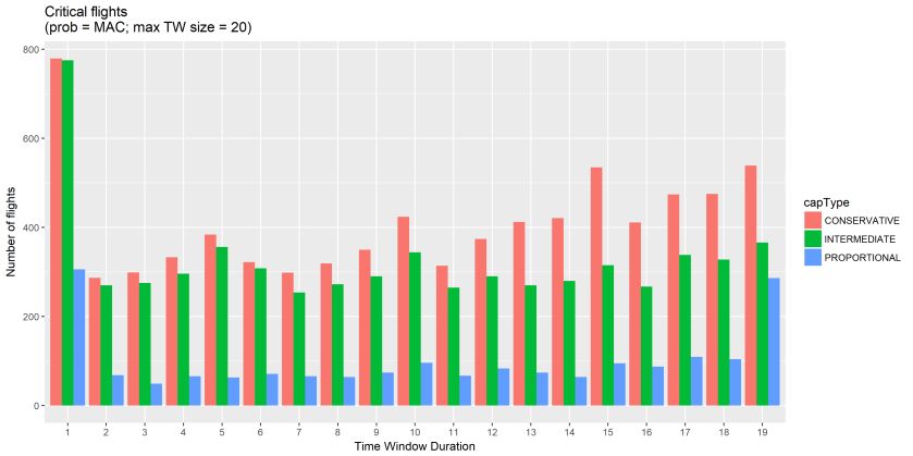
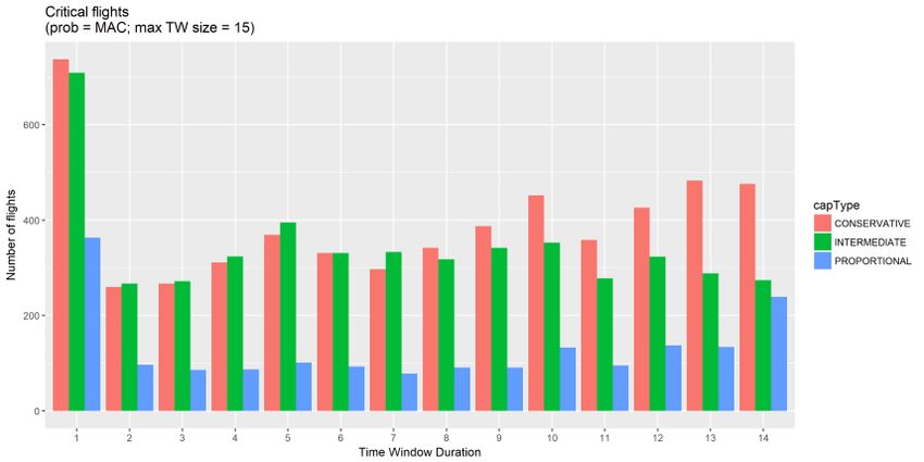
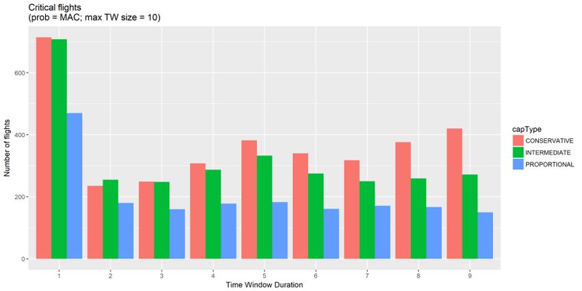
D3.1 FLIGHT FLEXIBILITY AND HOTSPOTS IN THE ADAPT SOLUTION

List of figures
Figure 1. Example of a trajectory and its sequence of time windows, red lines representing the shortest
time windows. .......................................................................................................................................... 9
Figure 2. Sectorisation configurations with one active sector (left) and two active sectors (right). .... 11
Figure 3. TW extending across two sector-hours. ................................................................................. 20
Figure 4. Proportion of constrained (critical) and flexible (non-critical) flights, depending on the
maximum TW duration (top TW=10 min, center TW=15min, bottom TW=20 min). ............................ 29
Figure 5. Number of constrained flights, divided by the assigned TW duration, across three model
variants (top, TW=10 min., center TW=15 min., bottom TW=20min.). ................................................ 30
Figure 6. Proportion of constrained (critical) and non-constrained flights in the conservative TW model,
for different minimum TW durations assigned (1,2, or 3 minutes). ...................................................... 31
Figure 7. Example of two flights constrained by four sector-hours: flight from LEMG to ESSA on the left,
flight from LEAM to EFHK on the right. .................................................................................................. 32
Figure 8. Proportion of non-constrained versus constrained flights. .................................................... 32
Figure 9. Sample of saturated sector-hours between 09:00 and 10:00. ............................................... 33
Figure 10. Sector that had a few significant capacity violations in the simulations for feasibility testing.
................................................................................................................................................................ 35
Figure 11. Proportion of constrained (critical) and non-constrained flights before (pre) and after (post)
capacity increase for the 5% of saturated sectors, for the intermediate TW model, with TWmax=15min.
................................................................................................................................................................ 37
Figure 12. Number constrained flights across the assigned TW duration, before and after the capacity
increase. ................................................................................................................................................. 37

List of tables
Table 1. Example of capacity utilisation coefficients ............................................................................. 23
Table 2. Run times of TW model variants for three different maximum TW durations. ...................... 28
Table 3. Percentage of sector-hours for which the capacity is violated. (Values averaged over 100 000
random instances) .................................................................................................................................. 34
Table 4. Criticality index for a sample of sector-hours (intermediate TW model, TWmax=15 min.) ...... 36

 5
 © – 2019 – Università degli Studi di Trieste, Technische Universiteit Delft,
 University of Westminster, Deep Blue, Università degli Studi di Palermo.
 All rights reserved. Licensed to the SESAR Joint Undertaking under conditions.
EDITION 01.01.00

Executive summary

The goal of the ADAPT strategic solution is to enhance the early flight planning, giving an indication of
how critical or flexible the execution of each flight can expect to be, and to indicate to which extent
the nominal capacity of each element of the network (i.e., sectors and airports) is going to be
respected.

The first phase of the development of the ADAPT solution, which is the formulation and
implementation of a deterministic model (European Strategic Flight Planning (ESFP) model) to define
flight trajectories and associated time windows at the strategic level, is presented in this deliverable.
The ESFP model builds on two deterministic, integer programming models. The first model, that we
term Strategic Air Traffic Assignment (SATA) model, was developed in the SATURN project, and its aim
is to assign a trajectory for each scheduled flight, in such a way that the nominal capacities of the
network are respected. When all flights have a trajectory and departure time assigned, these become
inputs of a second integer programming model, called Time Window (TW) model. This model uses
departure times as the starting position of each TW, and the objective is to guarantee the largest
flexibility by maximising the total duration of all TWs, i.e., the sum of the duration of all individual TWs.
The output of this second model are the trajectories, assigned TWs and the hotspots (saturated
elements) in the network.

Here we present the three variants of the TW model, which differ in the approach to accounting
capacity:

 1. Conservative, reserves a unit of capacity for any sector-hour the TW extends over, even though
 the flight will use only one unit of capacity in either of the two sector-hours.
 2. Proportional model, a fraction of unit of capacity is assigned to each period of TW duration,
 where the fraction is obtained by dividing the unit of capacity by the number of periods in the
 TW (duration).
 3. Intermediate, reserves the whole unit of capacity for the portion of the TW duration that falls
 within the first sector-hour, and a fraction of the unit of capacity for all the remaining periods
 of the TW that fall within the second sector-hour.
The EFPS model is run on a day of real air traffic data, encompassing the entire European Civil Aviation
Conference airspace. Different data items are needed to run the SATA and TW models, including
flights, airspace configuration, capacities of resources (sectors and airports), routes, aircraft types and
their operational costs, fuel costs, unit rates, and airline types. The data on air traffic and air network
structures are sourced from EUROCONTROL’s Demand Data Repository 2 (DDR2), for September 12th
2014. Cost data are taken from the report by (Cook & Tanner, 2015). In this deliverable we focus on
the results of the TW model. However, it is important to keep in mind that the SATA model is the input
of the TW model, thus the TW model results reflect the results of the SATA model as well.

6 © – 2019 – Università degli Studi di Trieste, Technische Universiteit
 Delft, University of Westminster, Deep Blue, Università degli Studi di
 Palermo. All rights reserved. Licensed to the SESAR Joint Undertaking
 under conditions.
D3.1 FLIGHT FLEXIBILITY AND HOTSPOTS IN THE ADAPT SOLUTION

The results show that the three TW models perform differently, proportional model being the one that
identifies the lowest number of constrained flights (those with TW lower than the TWmax), followed by
the intermediate model and closing with the conservative one. However, the proportional TW model
is also the slowest, and according to the outputs of the feasibility analysis could result in the highest
number of capacity violations. The results also change with the chosen TW duration – the longer is the
TW, more flights are identified as constrained.
Based on the results, the intermediate TW model is the preferred TW model: it reserves the capacity
in a less constraining manner than the conservative model, and results in less capacity violations than
the proportional TW model. We tested different TW durations – 10, 15 or 20 minutes. It is our opinion
that the TW of 15 minutes is most useful, as it requires less of unnecessary capacity reservations, and
is of the same length as the ATFM slots. However, as both the minimum and maximum durations of
TWs are the parameters of the model, they can always be changed.
The EFPS model assigns the trajectory, departure time and flexibility measure (TW) for all the flights in
the data instance (the ECAC network for the entire day of traffic). Apart from that, for each constrained
flight the limiting sector-hour is identified, which can be of help in case the airline user would prefer
to re-route the flight in order to increase its flexibility.
Furthermore, the TW model gives the list of saturated sector-hours throughout the day. Keep in mind
that the configurations are changed during the day. Having the information on the saturated sectors,
and their criticality index, the ANSPs could take mitigation actions in order to improve the situation.
For example, a supervisor having one or two saturated sectors, both with the low criticality index,
might decide that the current configuration is good enough as even if the capacity ends up being
violated it will be for a small number of flights, which in many cases is what already happens in every-
day operations. However, if there are few sector-hours within an ACC that have high criticality indexes,
the supervisor might decide to change the configuration into a one that brings more capacity.
As EFPS model is aimed at the strategic/pre-tactical flight planning phase, it can be used in the further
analysis of the system performance by different stakeholders – airlines, ANSPs, airports and Network
Manager. As the models are fast, they could also be used in the what-if scenarios, for example re-
routing or change of configuration.
It is important to note that even in the worst case (conservative TW model, TW of 20 minutes), about
25% of total daily flights are identified as constrained, out of which only a small portion (less than 3%
of total daily flights) are heavily constrained (TW of 1 minute). Most of other flights identified as
constrained still have some flexibility, and what is more, this flexibility is quantified – each flight is
assigned a TW of a certain duration.
Apart from the number of constrained flights, and their flexibility (assigned TW), TW models can
identify which are the network elements that impose limits on the flight’s flexibility, which can be
useful to airlines as well as to the air traffic control.

 7
 © – 2019 – Università degli Studi di Trieste, Technische Universiteit Delft,
 University of Westminster, Deep Blue, Università degli Studi di Palermo.
 All rights reserved. Licensed to the SESAR Joint Undertaking under conditions.
EDITION 01.01.00

1 Introduction

The goal of the ADAPT strategic solution is to enhance the early flight planning, giving an indication of
how critical or flexible the execution of each flight can expect to be, and to indicate to which extent
the nominal capacity of each element of the network (i.e., sectors and airports) is going to be
respected.

The ADAPT project consists of:

 1. Development of the ADAPT strategic solution.
 2. Tactical assessment.
 3. Visualisation.

The development of the ADAPT strategic solution consists of three phases:

1. the formulation and implementation of a deterministic model (European Strategic Flight
 Planning (ESFP) model) to define flight trajectories and associated time windows at the
 strategic level,
2. the assessment of the expected economic loss in case unwanted events occurring (e.g., flight
 delays, bad weather), and
3. the definition of some actions to mitigate on the day of operations expected demand and
 capacity imbalances, as detected in the two previous phases.

Phases 1 and 2 cover the definition of the ADAPT solution, while in phase 3 the outputs are used to
devise mitigation actions in order to improve the situation, if possible.

In this deliverable, phase 1 of the development of ADAPT strategic solution, the initial computational
experiments and obtained results are described. Phases 2 and 3 will be described, and their results
presented in D3.2, due in month 18 of the project.

The European Strategic Flight Planning (ESFP) model builds on two deterministic, integer programming
models. The first model, that we term Strategic Air Traffic Assignment (SATA) model, was developed
in the SATURN project (Bolic, et al., 2017) and was used in the extensive computational experiments,
taking into account a busy day in the European network, and the changing sectorisation. The aim of
this model is to assign a trajectory for each scheduled flight, in such a way that the nominal capacities
of the network are respected. When all flights have a trajectory and departure time assigned, these
become inputs of a second integer programming model, called Time Window (TW) model. This model

8 © – 2019 – Università degli Studi di Trieste, Technische Universiteit
 Delft, University of Westminster, Deep Blue, Università degli Studi di
 Palermo. All rights reserved. Licensed to the SESAR Joint Undertaking
 under conditions.
D3.1 FLIGHT FLEXIBILITY AND HOTSPOTS IN THE ADAPT SOLUTION

uses departure times as the starting position of each TW 1, and the objective is to guarantee the largest
flexibility by maximising the total duration of all TWs, i.e., the sum of the duration of all individual TWs.
The output of this second model are the trajectories, assigned TWs and the hotspots (saturated
elements) in the network.

1.1 Introducing Time Windows (TW)
To reconcile predictability with flexibility, we propose to express the flight flexibility in terms of time
windows, which are defined as time intervals associated with each flight segment (departure, arrival
or entry into a sector) - as depicted in Figure 1.

Figure 1. Example of a trajectory and its sequence of time windows, red lines representing the shortest time
 windows.

A TW is characterised by its position (opening time) and duration (equal to closing time - opening time).
In the context of strategic planning, the initial position of the time windows at departure and arrival
could coincide with the corresponding scheduled departure and arrival times, which are available
months before the actual day of operations. Scheduled times, however, are currently determined
without considering airspace capacities. In order to take the capacities into account, and determine
the time windows for flights, two steps, each corresponding to one of the two models, are taken.

First, the Strategic Air Traffic Assignment (SATA) model is applied, taking the changing sectorisations
and associated capacities into account, and proposes possibly needed shifts (within a predefined
threshold to comply with airport capacities and airspace users’ business requirements) or alternative
routes to meet them. A shift refers to moving the scheduled take-off or landing time to a time before
or after the scheduled one. In particular, this first model identifies, strategically, take-off and landing
times, and trajectories that minimise either the total shift or operational costs across all flights. Take-

1 A time window is a time interval describing the flexibility (in time dimension) of a trajectory. A time window indicates how “late” (with
respect to declared timing of the trajectory) a flight can be and still not create capacity-demand imbalances in the network.

 9
 © – 2019 – Università degli Studi di Trieste, Technische Universiteit Delft,
 University of Westminster, Deep Blue, Università degli Studi di Palermo.
 All rights reserved. Licensed to the SESAR Joint Undertaking under conditions.
EDITION 01.01.00

off time and trajectory information enable determining the times of entry into sectors along the
trajectory and finally the landing time. Thus, the opening time of each time window is set equal to the
corresponding take-off time, landing time or entry into a sector as computed in the Strategic Air Traffic
Assignment model. If each flight is operated so as to start the flight segments at the opening times of
the associated time windows, all airport and sector capacities are met, and the minimum total shift (or
operational costs) is achieved. In To grant the required flexibility, a flight might also be allowed to start
the flight segments after the assigned, precise times. In order to evaluate how much later these actions
can be performed, we use the TW model.

Thus, in the second step, the TW model is applied, giving as a result the duration of the time windows
for each flight. The TW model maximises the total duration of all TWs, thus looking for the maximum
flexibility for the flights in the system.

1.2 Introducing capacity matters
Current European ATM system offers a high level of flight planning flexibility, as only the final flight
plans need to be submitted several hours before departure. On the one hand, this allows airspace
users (AUs) the possibility to account for previously uncertain factors like weather forecasts, and thus
create flight plans that are most convenient for the day of operations. On the other hand, this flexibility
makes ATM system less predictable, resulting in costs due to flow measures, and under-utilisations
from a mismatch between available ATM capacity and traffic demand. The available ATM capacity on
the day of operations is often limited by the availability of the air traffic controllers.

When creating and subsequently submitting an initial flight plan, the airlines do not have the
information on airspace nominal capacities and do not need to consider it. Thus, a precise traffic load
on the airspace network is only known on the day of operations, while the capacity provision (e.g.
staffing levels) is usually planned starting more than a year ahead and is updated as time progresses.
On the day of operations in cases when available airspace (and airport) capacity cannot accommodate
planned air traffic, the ANSPs and Network Manager agree on the Air Traffic Flow Management (ATFM)
measures to reduce the demand on the congested parts of the network. The ATFM measures impose
delays on flights crossing congested network volumes (AUs can re-route around the area in question).
These delays and deviations are very costly to airlines (e.g. estimated to be more than 1B euro in 2014
(EUROCONTROL, 2017)).

Today, the airspace users do not need to consider the capacity of the airspace they would like to fly
through. However, the European ANSPs have the information on what is considered the nominal
capacity of each of the sectors under their jurisdiction. The actual capacity of an ANSP at each point in
time depends on the applied sectorisation. Figure 2 depicts two configurations2 of an ANSP: with just
one sector (left figure), and with two sectors, where the division is in the horizontal plane (right figure).
The nominal capacity of the first configuration is lower than that of the second one (42 compared to
95 entries in an hour).

2Configuration is a specific sectorisation. Airspace of each ANSP is divided in a number of elementary sectors.
There are different combinations of these elementary sectors – configurations that can be used in operations.
10 © – 2019 – Università degli Studi di Trieste, Technische Universiteit
 Delft, University of Westminster, Deep Blue, Università degli Studi di
 Palermo. All rights reserved. Licensed to the SESAR Joint Undertaking
 under conditions.
D3.1 FLIGHT FLEXIBILITY AND HOTSPOTS IN THE ADAPT SOLUTION

European definition of a capacity is the number of entries within the defined time horizon, usually an
hour. Thus, the nominal capacity defines how many flights can enter a sector during an hour, in
nominal conditions. The weather conditions can require effective lowering of the nominal capacity,
but that is done operationally, if there is a need for such measures (ATFM measures).

As the ADAPT models aim at the strategic/pre-tactical planning, hourly capacities are chosen, as they
are deemed detailed enough at this planning horizon. In the tactical setting, the hourly capacity is
usually considered too coarse and twenty-minute capacity is usually preferred. The EFPS model can
use either 60 or 20-minute capacities, and is already doing so in some cases as explained in the
following paragraphs. . However, focusing strictly on 20-minute capacities would increase the number
of constraints, which is already high, and may or may not translate into longer computational times.
More importantly, as the ADAPT is focused on improving strategic/pre-tactical planning, the 60-minute
capacities are considered to be good enough. Keep in mind that in the current strategic setting the
capacity figures are used very little by the ANSPs (when planning the traffic load, based on the historic
data), and not at all by the airlines.

 Figure 2. Sectorisation configurations with one active sector (left) and two active sectors (right).

The actual sectorisation is chosen by the supervisor based on the traffic demand prediction (short-
term prediction based on the submitted flight plans) and the staff availability. The changes are
actuated when the need arises, at any time of day.

Both optimisation models that are forming the ESFP model are formulated to include the capacity
constraints. As the most frequent capacity definition used is the hourly one, in our models we use
sector-hour capacity: hourly number of entries in the sector, when that particular sector is active. A
sector is active, when the configuration it belongs to is active.

As the configuration changes at need, the change can happen at any fraction of an hour. For example,
it can happen that a particular configuration is active from 8:00 to 10:20. In that case, the sectors
belonging to that configuration would have three sector-hour capacities assigned – two full sector-
hour capacities (from 08:00 to 10:00) and a partial sector-hour capacity where the hourly capacity is
scaled to 20 minutes.

 11
 © – 2019 – Università degli Studi di Trieste, Technische Universiteit Delft,
 University of Westminster, Deep Blue, Università degli Studi di Palermo.
 All rights reserved. Licensed to the SESAR Joint Undertaking under conditions.
EDITION 01.01.00

Furthermore, the ESFP models use the airport capacities as well. The airport capacities can be defined
for arrival, departure or general (mix of arrival and departure) operations. Here the capacity is given
as a number of such operations within a time period, usually an hour. For the sake of simplicity, we
often refer to these airport-hour capacities as sector-hour capacities.

12 © – 2019 – Università degli Studi di Trieste, Technische Universiteit
 Delft, University of Westminster, Deep Blue, Università degli Studi di
 Palermo. All rights reserved. Licensed to the SESAR Joint Undertaking
 under conditions.
D3.1 FLIGHT FLEXIBILITY AND HOTSPOTS IN THE ADAPT SOLUTION

2 EFPS Model

In this section the mathematical formulation of the two EFPS models (SATA and TW) is given. Both
models are centralised, meaning that all the needed information is collected in one place and the
system optimum is sought.

2.1 SATA - Strategic Air Traffic Assignment
The goal of SATA model is to re-distribute traffic demand in such a way that the nominal declared
capacities of network elements are respected. This model has been developed in the SATURN project
and its formulation and computational experiments are described in (Bolic, et al., 2017). This model is
a starting point of the EFPS model, and it is important the reader understands this first step, as it leads
to the second, Time Window model. Thus, in order to have formulations of both of the EFPS models,
we repeat the formulation of the model, as given in (Bolic, et al., 2017)
The SATA model has following characteristics:
 • Strategic shift of operations. As the model is applied in the strategic phase, before flight
 schedules are published, departure and arrival times earlier or later than the requested
 ones may be assigned. For this reason, when assigned times differ from requested times,
 we talk about schedule “shifts” rather than “delays”, which instead are dealt with in the
 tactical phase of operations. Thus, the assumption is that shifts assigned so much in
 advance would not impact the tail-number dependencies. However, the model
 specification includes the tail-number dependency constraint, which are not applied as we
 do not have access to the tail number data3.
 • Control of possible shift for airport movements. To avoid excessive shifting, the maximum
 allowed shift to earlier or later departure/arrival times is bounded.
 • No flight cancellations. All flights are assigned a strategic flight plan.
 • Departure time and route choice control. The model assigns the departure time and route
 for each flight. The route is chosen from the alternative routes specified by the airlines,
 with each route specifying the complete set of sectors to cross from origin to destination.
 Speed control is not taken into consideration, as it would make little sense in the strategic

3The additional notation and the tail-number dependency constraint for SATA model are given in the Appendix
A.

 13
 © – 2019 – Università degli Studi di Trieste, Technische Universiteit Delft,
 University of Westminster, Deep Blue, Università degli Studi di Palermo.
 All rights reserved. Licensed to the SESAR Joint Undertaking under conditions.
EDITION 01.01.00

 phase. Hence, the duration of each route is assumed to be constant, and sector entry and
 arrival times are uniquely identified for each route/departure time option.
 • Dynamic sectorisation. The configuration of the airspace changes throughout the day, and
 our model takes into account the evolution of sector openings/closures over the
 considered time horizon. A sector is considered active if it is open, inactive otherwise.
 • Re-entering a sector is allowed. Since flights may enter a sector more than once because
 of the sector shape or general airspace configuration, the formulation allows multiple
 entries in any sector.
 • Discrete time precision. The time horizon is subdivided into discrete time periods of size
 of choice.
 • Strategic capacity availability. Similarly to tactical capacity limitations in ATFM models,
 strategic (nominal) capacities for all flight actions, i.e., departure, arrival, and total airport
 movements , are defined, limiting the number of corresponding actions within a given time
 horizon (typically one hour). The same applies to sectors, where capacity limits the number
 of possible entries in a time horizon, following the European definition of sector capacity.

2.1.1 Notation for SATA model
The notation is the following:

F set of flights, indexed by f
K set of airports, indexed by k
A set of aircraft types, indexed by a
 aircraft type used to perform flight f
O set of origin-destination (OD) pairs, indexed by o
 OD pair connected by flight f
 set of sectors, indexed by s
R set of routes, indexed by r
 ⊆ set of routes that may be used by a flight operating between OD pair o with aircraft
 type a
 number of elements (sectors and airports) along route r
 i-th element (airport or sector) of route r
B set of flight actions, B = {ent, dep, arr, tot }, where ent is an entry into a sector, and
dep, arr, and tot are departure, arrival, and total (i.e., departure or arrival) airport movements,
respectively
T set of time periods at which flight actions are considered
E set of elements ∪ (sectors and airports), indexed by j

H set of hours, indexed by h
 ℎ set of time periods in hour h in which element j is active
 ℎ
 , maximum number of flights that may perform action b at element j in hour h (i.e.,
 capacity)
 requested departure time of flight f

14 © – 2019 – Università degli Studi di Trieste, Technische Universiteit
 Delft, University of Westminster, Deep Blue, Università degli Studi di
 Palermo. All rights reserved. Licensed to the SESAR Joint Undertaking
 under conditions.
D3.1 FLIGHT FLEXIBILITY AND HOTSPOTS IN THE ADAPT SOLUTION
requested arrival time of flight f
Tfr set of time periods allowed for departure for flight f along route r
origin airport of OD pair o
destination airport of OD pair o
flight time from origin to the i-th element of route r
The trajectory of a flight is defined through a route ∈ . All the sectors that a flight may traverse
following route r are given in the structure, where they are sequenced on the order in which a flight
traverses them. The time of execution of a flight action (i.e., departure, arrival, or sector entry) is
identified by flight f ∈ F and element index i ∈ [1, nr ]. This is different from the formulation commonly
adopted in ATFM models, where trajectories are identified in terms of flight f and airport/sector ∈
S ∪ K only (see for example Bertsimas et al., 2011).
2.1.2 Decision variables
The following set of decision variables is used in the proposed model:
1, if flight f departs at time period t following
( ) = { route r;
∀ ∈ , ∈ , ∈ (1)
0,
otherwise.
The decision variables represent the assignment, as allocated by the central planner, of departure time
t and route r, for each flight. Since all flights are assigned a departure time and route (i.e., no flights
are cancelled), only one decision variable per each flight will be equal to 1, and all other variables will
be equal to 0.
2.1.3 Objective functions
Strategic flight plans can be obtained using two alternative objectives:
• Shift minimisation (MS – minimum shift): the total schedule shift of flights is minimised.
• Flight operational cost minimisation (MC – minimum cost): the total operational cost of
flights is minimised.
2.1.3.1 Shift-based objective function
The shift-minimisation objective function sums the negative departure and positive arrival shifts per
flight. These are the minutes of earlier-than requested departures and later-than requested arrivals
respectively. Such a definition prevents from counting twice the shift that is propagated from
departure to arrival or vice-versa.
To guarantee equity in the assignment of strategic flight plans, we adopt the well-known approach
used by Lulli and Odoni (2007). Their approach ensures equity by including in the objective function
cost coefficients that are a superlinear function of the quantity that should originally be minimised for
each flight (in their case the tardiness of a flight, in our case the flight shift). That is, instead of
15
© – 2019 – Università degli Studi di Trieste, Technische Universiteit Delft,
University of Westminster, Deep Blue, Università degli Studi di Palermo.
All rights reserved. Licensed to the SESAR Joint Undertaking under conditions.EDITION 01.01.00
minimising the summation over all flights of some coefficients , these coefficients are accounted for
1+
under the form 1 , with 1 > 0 and close to zero (Bertsimas and Gupta, 2016). The use of these
coefficients favours “the assignment of a moderate amount of delay to each of two flights rather than
the assignment of a small amount to one and a large amount to the other” (Lulli and Odoni, 2007).
Given some 1 > 0, the objective function is thus formalised as follows:
1+ 1
∑ ∑ ( ) ⋅ (max { − , 0} + max { + + − , 0}) (2)
∈
∈ , ∈
( )
The two terms multiplied by ( ) describe the assigned departure negative shift and arrival positive
shift, respectively. For simplicity, the departure negative and arrival positive shifts are referred to as
“departure shift” and “arrival shift” in the following text.
2.1.3.2 Cost-based objective function
The cost-minimisation objective function aims at minimising flights’ strategic operational costs. These
are all the costs that can be accounted for in advance and consist of ground and airborne operation
costs, and en route charges. The estimation of the strategic unit ground and airborne costs is based on
the strategic coefficients and values defined in the report by (Cook & Tanner, 2015).
• Strategic ground costs are calculated as the unit ground cost ( : cost of one minute of
ground operation of aircraft type a) times the undesired amount of time the flight has to
remain grounded, i.e., the shift . These costs include ground maintenance, fleet and crew
utilisation costs (Cook and Tanner, 2015. Table 9).
• Strategic airborne costs are calculated as the unit airborne cost ( : cost of one minute of
airborne operation of aircraft type a) times the flight duration ( ). These costs include
airborne maintenance, fleet and crew utilisation, and fuel costs (Cook and Tanner, 2015, Table
11).
• Route charges ( : route charges for a flight operated by aircraft type a on route r) are the
means of financing of European ANSPs, and are levied for each flight in the European airspace.
They are calculated as the product of the distance factor (distance flown in ANSP’s airspace),
weight factor, and the unit rate (which varies across ANSPs), as defined by EUROCONTROL’s
Central Route Charges Office (2015).
Hence, similarly to other approaches already proposed in literature (see for example Bertsimas et al.,
2011 and Castelli et al., 2013), the strategic cost to operate a flight with aircraft type a along route r
with minutes of shift ( ( )) is calculated as follows:
( )= ⋅ + ⋅ + (3)
To guarantee equity, we follow the same approach as that used in the MS objective function, using
superlinear cost coefficients by raising flight costs to the power of 1 + 2 , with 2 > 0 and close to
zero. The cost-based objective function of the problem is then:
16 © – 2019 – Università degli Studi di Trieste, Technische Universiteit
Delft, University of Westminster, Deep Blue, Università degli Studi di
Palermo. All rights reserved. Licensed to the SESAR Joint Undertaking
under conditions.D3.1 FLIGHT FLEXIBILITY AND HOTSPOTS IN THE ADAPT SOLUTION
1+ 2
∑ (| − |) ⋅ ( )
(4)
∈ , ∈ , ∈
2.1.4 Constraints
The SATA model has the following constraints:
∑ ( ) ≤ ,
ℎ ∀ ∈ , ℎ ∈ (5)
∈ , ∈ ∶ = ,
∈ ℎ
∑ ( ) ≤ ,
ℎ ∀ ∈ , ℎ ∈ (6)
∈ , ∈ ∶ = ,
+ ∈ ℎ
∑
( ) + ∑
ℎ
( ) ≤ , ∀ ∈ , ℎ ∈ (7)
∈ , ∈ ∶ = , ∈ , ∈ ∶ = ,
∈ ℎ
+ ∈ ℎ
∑ ( ) ≤ ,
ℎ ∀ ∈ , ℎ ∈ (8)
∈ , ∈ ,
∈[2, −1]: = ,
+ ∈ ℎ
∑ ( ) = 1 ∀ ∈ (9)
∈ , ∈
( ) ∈ {0, 1} ∀ ∈ , ∈ , ∈ (10)
Constraints (5), (6), and (7) enforce the departure, arrival, and total airport capacity constraints,
respectively. Total airport movements include both departures and arrivals. Similarly, sector capacity
constraints are defined by (8). Since the formulation we propose takes into account the dynamic
configuration of the airspace, capacity constraints are defined only for active sectors. Each sector may
open and close several times during a day, and each opening interval is defined by the set, which
includes all time instants in the i-th opening of sector j. Finally, equations (9) and (10) enforce the
choice of a single departure time instant and route for each flight, provided that the decision variables
( ) are binary.
17
© – 2019 – Università degli Studi di Trieste, Technische Universiteit Delft,
University of Westminster, Deep Blue, Università degli Studi di Palermo.
All rights reserved. Licensed to the SESAR Joint Undertaking under conditions.EDITION 01.01.00
2.2 Time Windows model
The Time Windows is based on the same characteristics as the SATA model (see section 2.1)4.
2.2.1 Notation
The notation used to define the model is the following:
≡ set of airports, indexed by a,
≡ set of sectors, indexed by ,
≡ ∪ set of airports, and sectors, indexed by ,
≡ set of flights, indexed by ,
≡ departure airport of flight ,
≡ destination airport of flight ,
≡ set of routes, indexed by , where is a chosen route for a flight ,
≡ number of elements (airports and sectors) along the chosen route ,
≡ -th element of the route ,
≡ flight time from origin to the -th element of route ,
≡ scheduled departure time of flight , i.e. the position of the departure TW,
≡ minimum duration of each TW,
≡ maximum duration of each TW,
≡ { + 1 , … , + + − 1 }
≡ set of feasible time periods for flight , to arrive at the -th element of the route ,
≡ { , , , }
≡ set of actions that can be performed by a flight, , , stand for arrival, departure or
generic movement type at an airport, and stands for entry into a sector,
≡ set of sector-hours linked with the action at sector or airport , indexed by ,
≡ opening time period of sector-hour , (i.e. opening time of a sector ),
≡ closing time period of sector-hour ,
≡ { , … , − 1}
≡ set of time periods during which the sector-hour is active,
4TW model formulation includes the turnaround (tail-number dependency) constraints, as the SATA model, and
those are given in the Appendix A.
18 © – 2019 – Università degli Studi di Trieste, Technische Universiteit
Delft, University of Westminster, Deep Blue, Università degli Studi di
Palermo. All rights reserved. Licensed to the SESAR Joint Undertaking
under conditions.D3.1 FLIGHT FLEXIBILITY AND HOTSPOTS IN THE ADAPT SOLUTION
≡ capacity enforced during sector-hour , (i.e. declared capacity of a sector , during the sector-
hour )
2.2.2 Decision variables
Decision variables are used to capture the duration of departure Time Window for each flight:
1, if the TW for flight f is still open for departure
( ) = { at time t; ∀ ∈ , ∈ 0 (11)
0, otherwise.
2.2.3 Objective function
The objective function maximises the total duration of all TWs:
max ∑ ( ) ∙ ( − )
(12)
∈ , ∈ 0
Cost coefficients ensure that TW durations are distributed as fairly as possible, i.e. the model will
favour the assignment of TWs of similar duration to each of two flights, rather than the assignment of
a large TW to one flight and a small one to another.
( ) = 1 − , 0 ≤ ≤ − 1
∙| | (13)
2.2.4 Constraints
2.2.4.1 Definition constraints for decision variables
Decision variables ( ) are binary, monotone decreasing variables.
( ) ≥ ( + 1), ∀ ∈ , ∈ 0
(14)
( ) ∈ {0, 1}, ∀ ∈ , ∈ 0
(15)
2.2.4.2 Time Window duration constraints
There are two TW duration constraints – minimum and maximum duration constraints. The minimum
duration constraint guarantees that the specified minimum duration for TWs is respected, by taking
advantage of the fact that decision variables are monotone decreasing as imposed by constraint 14.
( + − 1) = 1, ∀ ∈
(16)
19
© – 2019 – Università degli Studi di Trieste, Technische Universiteit Delft,
University of Westminster, Deep Blue, Università degli Studi di Palermo.
All rights reserved. Licensed to the SESAR Joint Undertaking under conditions.EDITION 01.01.00
The maximum duration constraint defines the set containing a number of time periods that is equal
to the maximum TW duration .
≡ { + , … , + + − 1 }
2.2.4.3 Capacity constraints
Capacity constraints ensure that sector and airport capacities are respected for all sector-hours. As
was already mentioned, the capacity is defined as the number of entries into the sector during an hour.
If the trajectories assigned by the SATA model are flown with the accuracy of one minute, then all the
sector-hour capacities defined in the network are respected. However, the point of the TW model is
to determine how much flexibility in terms of time can be assigned to each trajectory. To be able to
optimally assign the TWs, we need to take into account the possibility that the TW can extend into the
following sector-hour, as depicted in Figure 3. The depicted trajectory is planned to enter the blue
sector at 8:55 (sector-hour 8 – SH8), respecting the capacity. If there are no other flights scheduled to
enter the sector and/or there is spare nominal capacity, we can assign 5 minutes of flexibility to this
flight.
08:55
TW
SH8 SH9
08:00 09:00 10:00
Figure 3. TW extending across two sector-hours.
In order to extend the TW for more than 5 minutes, we will need to reserve one unit of capacity in the
following sector-hour (SH9) for the duration of TW.
20 © – 2019 – Università degli Studi di Trieste, Technische Universiteit
Delft, University of Westminster, Deep Blue, Università degli Studi di
Palermo. All rights reserved. Licensed to the SESAR Joint Undertaking
under conditions.D3.1 FLIGHT FLEXIBILITY AND HOTSPOTS IN THE ADAPT SOLUTION With that in mind, to simplify the definition of capacity constraints, we use additional logic parameters: • , ( ) determines whether time period is the first period of TW, or the first period of opening of the sector-hour : ( ) , ≔ ( = + ) ⋁( = ) • ( ) determines whether the TW for flight , that may reserve capacity in sector-hour , in the −th element of its route, starts before the opening of sector-hour : ( ) ≔ + < < + + − 1 • ( ) determines whether the TW for flight , that may reserve capacity in sector-hour , in the -th element of its route ends after the closure of sector-hour : ( ) ≔ + < < + + − 1 Thus, the capacity constraints can be expressed as: ∑ ∈ , ∈ : ( ) ≤ , ∀ ∈ , ∈ 0 ( ) = ⋀ , (17) −1 ∑ ( − ) ≤ , ∀ ∈ , ∈ ∈ , ∈ : −1 (18) = ⋀ , ( ) −1 ∑ ∈ , ∈ : ( ) + ∑ ∈ , ∈ : ( − ) ≤ , ∀ ∈ , ∈ 0 ( ) −1 = ⋀ , = ⋀ , ( ) (19) −1 ∑ ( − ) ≤ , ∀ ∈ , ∈ ∈ , ∈[1, −2]: = ⋀ , ( ) (20) The constraint (17) imposes the departure capacity at the airport (if defined), the constraint (18) the arrival and constraint (19) the general airport capacity. The constraint (20) imposes sector capacity. 21 © – 2019 – Università degli Studi di Trieste, Technische Universiteit Delft, University of Westminster, Deep Blue, Università degli Studi di Palermo. All rights reserved. Licensed to the SESAR Joint Undertaking under conditions.
EDITION 01.01.00

2.3 Variants of TW model
2.3.1 Conservative TW model
Previous section (section 2.2) presents the initial version of the TW model, that we term the
conservative model. The model described above could lead to overly conservative solutions since it
may reserve an excessive amount of capacity for each flight: in case a TW extends over two sector-
hours (see Figure 3), the model reserves a whole unit of capacity, even though the flight will use only
one unit of capacity in either of the two sector-hours.
(Castelli, et al., 2011) presented two alternative approaches to computing the utilisation of the
capacity in order to avoid too conservative solutions. Adopting the reasoning by Castelli et al, we
develop two further variants of the TW model:
 • Proportional model;
 • Intermediate model.
These two model variants are obtained by varying the capacity constraints 17, 18, 19 and 20 presented
above.

2.3.2 Proportional TW model
Proportional model. In this variant, a fraction of unit of capacity is assigned to each period of TW
duration, where the fraction is obtained by dividing the unit of capacity by the number of periods in
the TW (duration). As an example, if there is a 5-period TW, two of which are within the sector-hour
 1, and the remaining three are within the sector-hour 2, only 2⁄5 of the unit of capacity will be
reserved in sector-hour 1, and the 3⁄5 will be reserved in 2.
To put this in practice, as the TW duration is determined in the optimisation model, we introduce the
following:
 • as the capacity utilisation coefficient for each period of the TW duration, [0, 1];
 • as the number of periods of the TW falling within the first sector-hour;
 • as (any) remaining periods of TW falling within the second sector-hour. ∈ [ ; − 1]
Thus, the new capacity utilisation coefficients ( , ), ≥ are defined as follows:
 1
 , if = ;
 +1
 ( , ) = ∀ , ∈ [0; − 1], ≥ (21)

 , if >
 { ( + 1)
Table 1 shows an example of the capacity utilisation coefficients ( , ) for the TW of the duration 5
( = 5).

22 © – 2019 – Università degli Studi di Trieste, Technische Universiteit
 Delft, University of Westminster, Deep Blue, Università degli Studi di
 Palermo. All rights reserved. Licensed to the SESAR Joint Undertaking
 under conditions.
D3.1 FLIGHT FLEXIBILITY AND HOTSPOTS IN THE ADAPT SOLUTION Table 1. Example of capacity utilisation coefficients =0 =1 =2 =3 =4 =0 1 0 0 0 0 =1 1 1 1 1 2 6 12 20 =2 1 1 1 3 6 10 =3 1 3 4 20 =4 1 5 Thus, in the proportional model, the constraint 17 becomes: ∑ ( − ( + ), − ( + )) ∙ ( − ) ∈ , ∈[1, −2], ∈ ⋂ : (22) = ⋀ ( ) + ∑ ( − ) ∈ , ∈[1, −2], ∈ : ( ) ¬ ( ) = ⋀ , ⋀ − ∑ ( − ( + ), − ( + )) ∙ ( − ) ≤ , ∈ , ∈[1, −2], ∈ \ : = ⋀ ( ) ∀ ∈ , ∈ 2.3.3 Intermediate TW model In this variation of the TW model, we reserve the whole unit of capacity for the portion of the TW duration that falls within the first sector-hour, and a fraction of the unit of capacity for all the remaining periods of the TW that fall within the second sector-hour. Taking up the previous example, if there is a 5-period TW, two of which are within the sector-hour 1, and the remaining three are within the 23 © – 2019 – Università degli Studi di Trieste, Technische Universiteit Delft, University of Westminster, Deep Blue, Università degli Studi di Palermo. All rights reserved. Licensed to the SESAR Joint Undertaking under conditions.
EDITION 01.01.00

sector-hour 2, one unit of capacity will be reserved in sector-hour 1, and the 3⁄5 of the capacity unit
will be reserved in 2.
Thus, the capacity constraint 20 from the conservative TW model becomes:

 ∑ ( − ( + ), − ( + )) ∙ ( − )
 ∈ , ∈[1, −2], ∈ ⋂ : (23)
 = ⋀ ( )

 +∑ ∈ , ∈[1, −2], ∈ : ( − ),∀ ∈ , ∈
 ( )
 = ⋀ , ⋀ ¬ ( )

Note that the constraint 23 does not contain the last negative component of the constraint 22 of the
proportional model.

 − ∑ ( − ( + ), − ( + )) ∙ ( − ) ≤ ,
 ∈ , ∈[1, −2], ∈ \ :
 = ⋀ ( )

This component has the task of discounting the amount of capacity of an sector-hour reserved for
those flights that enter the sector in the a subsequent sector-hour because the relative time window
ends after the closure of sector-hour (and opening of the sector-hour 1).

24 © – 2019 – Università degli Studi di Trieste, Technische Universiteit
 Delft, University of Westminster, Deep Blue, Università degli Studi di
 Palermo. All rights reserved. Licensed to the SESAR Joint Undertaking
 under conditions.
You can also read