Understanding Cycling Mobility: Bologna Case Study - arXiv
←
→
Page content transcription
If your browser does not render page correctly, please read the page content below
Understanding Cycling Mobility: Bologna Case
                                                                 Study
                                                     Taron Davtian                                   Flavio Bertini                                  Rajesh Sharma
                                             Institute of Computer Science           Department of Mathematical, Physical and                  Institute of Computer Science
                                                    University of Tartu               Computer Sciences, University of Parma                          University of Tartu
                                                      Tartu, Estonia                               Parma, Italy                                         Tartu, Estonia
                                                   taron.davtian@ut.ee                        flavio.bertini@unipr.it                                rajesh.sharma@ut.ee
arXiv:2109.04243v1 [cs.CY] 9 Sep 2021

                                           Abstract—Understanding       human      mobility    in    urban        Like many other cities, Bologna -a historical and a uni-
                                        environments is of the utmost importance to manage traffic             versity city in Italy- struggles to manage urban traffic and
                                        and for deploying new resources and services. In recent years,         its side-effect, such as CO2 emissions. In 2017, the Public
                                        the problem is exacerbated due to rapid urbanization and
                                        climate changes. In an urban context, human mobility has many          Transport Authority SRM Reti e Mobilità Srl1 promoted the six
                                        facets, and cycling represents one of the most eco-friendly and        months Bella Mossa2 initiative through which it encouraged
                                        efficient/effective ways to move in touristic and historical cities.   eco-friendly means of transportation and reduced day-to-day
                                        The main objective of this work is to study the cycling mobility       reliance on single-occupancy car journeys. The program was
                                        within the city of Bologna, Italy. We used six months dataset          intended to reward users with points (to be transformed into
                                        that consists of 320,118 self-reported bike trips. In particular,
                                        we performed several descriptive analysis to understand spatial        prizes later) for walking, cycling, and using public transport.
                                        and temporal patterns of bike users for understanding popular          In particular, through a mobile application, the users chose
                                        roads, and most favorite points within the city. This analysis         the type of activity they were about to perform, and the
                                        involved several other public datasets in order to explore             application started tracking and recording positions via the
                                        variables that can possibly affect the cycling activity, such as       users’ smartphone GPS. In this study, we focused on cycling
                                        weather, pollution, and events. The main results of this study
                                        indicate that bike usage is more correlated to temperature, and        mobility due to the wider coverage of the city offered by
                                        precipitation and has no correlation to wind speed and pollution.      this means of transportation (e.g., short/long trips, small/large
                                        In addition, we also exploited various machine learning and            streets).
                                        deep learning approaches for predicting short-term trips in the           To understand cycling mobility, we analyzed bike usage
                                        near future (that is for the following 30, and 60 minutes), that
                                        could help local governmental agencies for urban planning. Our         through the 320,118 self-reported unique bicycle trips in the
                                        best model achieved an R square of 0.91, a Mean Absolute               city of Bologna within the Bella Mossa dataset. These trips
                                        Error of 5.38 and a Root Mean Squared Error of 8.12 for the            span across six months period, starting from April 2017 to
                                        30-minutes time interval.                                              September 2017. In particular, the study covers the following
                                                                                                               aspects:
                                        keywords: Cycling mobility, Geo-referenced data analysis,
                                        Big data, Short-term mobility forecasting, Machine Learning.             1) Temporal analysis: We evaluated how the cycling
                                                                                                                    mobility changes during days, weeks and months, and
                                                               I. I NTRODUCTION                                     computed the average speed, length, and travel times of
                                           In recent years, the possibility of geo-referenced data collec-          the trips to understand the temporal characteristics of the
                                        tion has opened doors for understanding human behaviour in                  cycling mobility.
                                        urban contexts, such as pedestrian mobility [1], taxi services           2) Spatial analysis: We reconstructed the utilization map
                                        [2] and bike and scooter-sharing mobility [3]. In particular,               of the city’s road network highlighting popular roads and
                                        bike-sharing services offer new opportunities for researchers               most favorite points within the city. The identification of
                                        to study human mobility by analyzing spatial patterns [4] and               the points of interest and routes used by users made it
                                        temporal patterns [5] of bike usage or by studying the effects              possible to study how people spread out from the main
                                        of weather on bike-sharing services [6].                                    identified locations.
                                           Local governments promote cycling as an eco-friendly and              3) External variables: To the best of our knowledge, when
                                        healthy means of local transportation due to the significantly              analyzing bike usage the studies in literature focused
                                        growing awareness about climate change and its capability                   on a single aspect such as by either understanding the
                                        in lightening road traffic within touristic and historical cities.          impact of weather conditions [7] or analysing temporal
                                        However, to identify the transport demand of cyclists and                   patterns [5]. However, we considered several variables
                                        to quantify the utilization of the road represent the main
                                        challenges to improve infrastructures (e.g., bike lanes and              1 http://www.srmbologna.it

                                        racks) and manage traffic.                                               2 https://www.bellamossa.it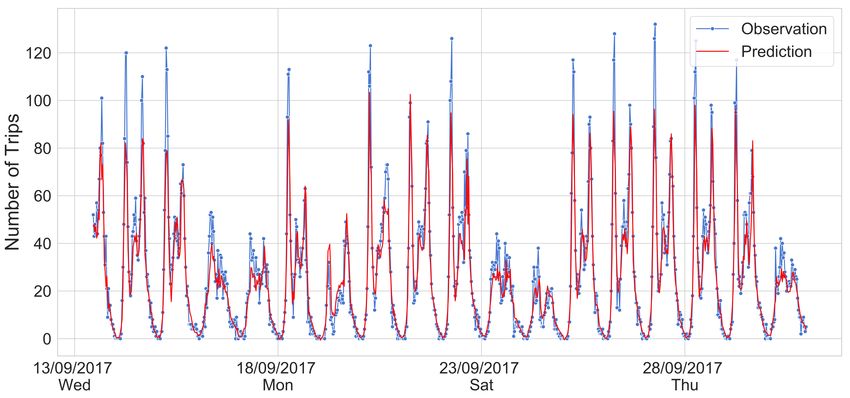
that can affect cycling mobility, such as weather, pollu-          and the authors indicated that the result confirms other prior
     tion, seasonality, holidays, and events.                           researches [12], [13].
  4) Predictive analysis: We used machine learning and                     Some other works analysed bike usage across different parts
     deep learning approaches to forecast the number of                 of the cities. For example, in [14] Froehlich et. al. investigated
     trips for the near future, that is, in the next i) 30              behaviors of bike users across different locations and times
     minutes, and ii) 60 minutes to study daily bicycle traffic         of the day in Barcelona’s neighborhood. In [15], the authors
     trends that could possibly help in traffic management              explored the bike-sharing travel time and trips by gender and
     and infrastructures deployment.                                    day of the week. The results of the study suggested that
   The paper is structured as follows. Section II outlines the          demand for bike usage is generated in the residential districts,
current state of knowledge within which this study falls.               while the biggest hubs are train stations. The paper showed
Section III presents a detailed description of the datasets.            that there is a big difference in the sense of distance and trip
In Section IV, we discuss the descriptive analysis results              duration between men and women. Additionally, the authors
using the cycling dataset and other datasets about weather,             reported that women are using bikes during weekdays more,
pollution, and events. Section V presents the methodology               while men use it on average more during weekends. In another
and experimental results on short-term mobility forecasting.            paper, researchers examined the behavior of bike usage in the
Finally, some concluding remarks and future works are made              city of Lyon, France, by focusing on how social behavior help
in Section VI.                                                          in planning and designing policies in transportation [16].
                                                                           In this work, we analysed how different indicators such as i)
                    II. R ELATED WORKS                                  air pollution, ii) weather conditions, iii) temperature affect bike
                                                                        usage. In addition, we also analysed the spatial and temporal
   In this section, we examine works that have studied bike             dynamics of bicycle usage in order to provide a holistic picture
mobility. Firstly we discuss papers that have investigated the          of cycling mobility.
behaviors of the bike users (Section II-A). Then, we examine
the papers where authors have performed predict analysis for            B. Predictions using bike data
different tasks, such as for distributing bikes in the city for            The second line of our research has been conducted about
easier usage or traffic flow (Section II-B).                            predicting the usage of bikes by exploring various machine
                                                                        learning algorithms. In [17], authors analyzed operational data
A. Analyzing bike usage
                                                                        from bike-sharing systems to understand activity patterns and
   Numerous studies have been done in order to understand               to use these patterns in order to plan the distribution of bikes.
the effect of weather on the use of bicycles. For example, in           A hierarchical prediction model was employed in [18] with
[7], the research was conducted on how weather conditions               an aim to predict the number of bikes that are rented from
affect the usage of bikes in the city of Cork, Ireland: trips are       each station to meet the demand. In contrast, Xu et al. [17]
shorter during rains, and longer trips are done during sunny            used a hybrid prediction model by combining clustering with a
days. In [6], the authors found that precipitation in a single          support vector machine for predicting bicycle traffic flow. In a
hour might significantly affect the number of bike trips. They          different work [19], the authors tried to predict the destination
also noted that cycling during weekends is more affected by             and arrival time of each bicycle trip, which can effectively help
weather than during weekdays. El-Assi et al. [8] studied how            the companies to move bikes on time for the under-supplied
weather affects bike sharing demand in the second biggest               station.
city of Canada, Toronto. The findings implied that there is a              In some recent works, a deep learning approach has been
significant correlation between air temperature and bike usage.         used in order to forecast bike demand. Some of them experi-
Authors also investigated how the built environment affects             mented with large-scale datasets and tried to predict demand
bike demand, concluding that bike infrastructure plays a major          for different time intervals using only historical bike usage
role in increasing the popularity of bike usage. Nankervis [9]          data [20], [21]. Zhang et al. [22] used Long Short-Term
found out in their study that weather’s both short-term (e.g.           Memory (LSTM) model to predict the number of trips by also
daily temperature) and long-term (e.g. seasonal conditions)             considering public transport usage. For predicting the facility
affect bike usage significantly. Similarly, in [10], researchers        choice of cyclists between on-street and off-street facilities, a
discussed how seasonal factors affect bicycle commuting. The            machine learning model was developed by authors of [23]. In
results of the study confirmed that there is a high correlation         another work, along with the usage of weather data, taxi usage
between weather and bike usage.                                         was also explored for predicting bike trips for the city of New
   Some other studies focus on the impact of infrastructure             York [24].
on bike usage. For example, in [5], the authors investigated               Recently, a number of studies have also investigated dock-
which road attributes influence bike users’ path choices. In            less bike-sharing systems [25], [26], [27]. The main emphasis
[11], researchers in Melbourne and Brisbane tried to quantify           is on analysing spatial patterns of such systems, as without
the factors influencing bike-share membership through a ques-           stations, bicycles can be left anywhere in the city, which
tionnaire. The results showed that the distance to the closest          also raises the question of redistribution of bikes in particular
docking station is highly correlated with the membership                during the weekdays [4], [28], [29]. These papers have focused

                                                                    2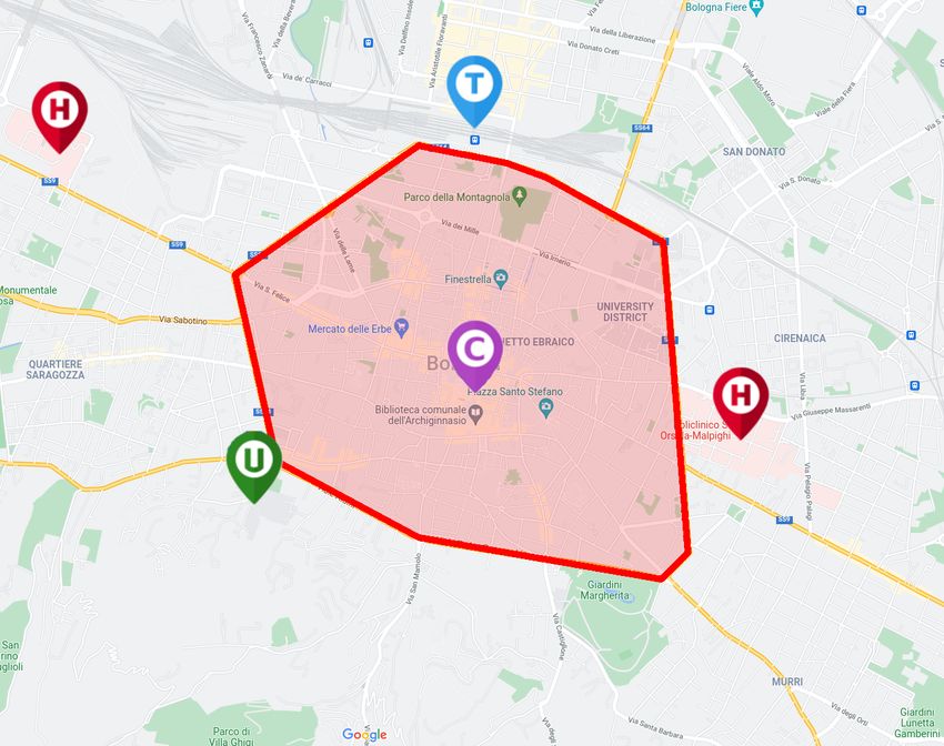
mainly on the problem of redistribution of the bikes in different       B. Supplementary data sources
locations. In addition, they tried to predict the locations where          Besides the main dataset, we used several supplementary
there will be a surplus of bikes as well as locations having a          datasets for analyzing bike usage and predicting the number
shortage of bikes. In this work, we tried to predict the number         of bike trips.
of trips by not only considering the historical bike usage data         1) Weather: We downloaded historical data about tempera-
but also air temperature, precipitation, holidays, and events.          ture, precipitation, and wind for the observation period for
                                                                        the city of Bologna from the website of the Regional Agency
                         III. DATSETS                                   for Prevention, Environment, and Energy3 of Emilia-Romagna,
   This section of the paper provides information about the             Italy. The dataset contains information about the hourly aver-
datasets we used for the analysis. In particular, we describe           age air temperature above 2 meters from the ground, the hourly
the Bella Mossa 2017 dataset about self-reported bike usage,            average wind speed above 10 meters from the ground, and the
and the other supplementary data sources (weather, pollution,           cumulative precipitation data over 1 hour period.
events, etc.) that were used for our analysis.                          2) Pollution: We used the information about pollution from
                                                                        the website of the Ministry of Economic Development4 in
A. Bella Mossa 2017 dataset                                             Italy. Based on the 2005 World Health Organization (WHO)
                                                                        Air Quality Guidelines5 , we analysed four main air pollution
   The main dataset used in the paper contains mobility data            indicators, that is i) Particulate matter (PM), ii) Ozone (O3),
of different transportation means for the period of six months,         iii) Nitrogen dioxide (NO2), and iv) Sulfur dioxide (SO2).
that is, from April 1, 2017 to September 30, 2017. Bella                3) Holidays and events: We used publicly available informa-
Mossa was an initiative promoting a healthy lifestyle and               tion about the holidays in Italy and public events in the city
sustainable mobility among users residing in Bologna, Italy.            of Bologna6 . The dataset contains information about public
It gave the user a chance to win various gifts and discounts            holidays, national celebration days, and civil solemnities in
as a reward for using a more sustainable and healthy means              the city of Bologna. Also, we gathered information about
of transportation. For participating, a user just needed to             strikes and protests for the observation period for the city of
download the mobile application and started it whenever they            Bologna7 .
go out for a walk, use bikes, trains, buses, or even when using
carpooling. The running application tracked and stored data                                  IV. D ESCRIPTIVE A NALYSIS
related to the users’ position using the GPS of the users’                 In this section, we present the results of the descriptive
smartphone. During the six months of the program, there were            analysis of the Bella Mossa bike data. Firstly, we present the
over 15,000 unique users who registered for this program,               results of the temporal analysis looking into daily, monthly
and 3.7 million Km was covered by them during 895,000                   and seasonal trends of bike usage (Section IV-A). Then, we
journeys. For security reasons, the dataset does not include            show the spatial analysis results to highlight which parts of
users’ personal information, and thus, we could not distinguish         the city attract most of the bike trips (Section IV-B). Next, we
and analyze different patterns considering users gender or age.         present the results by combining the cycling mobility data with
Moreover, the data is anonymised, and it is worth noting that           the supplementary data sources. In particular, we discuss how
each trip in the dataset is identified by a unique identification       weather conditions, such as a change in air temperature and
number (ID), however, this ID does not allow users to be                precipitation, correlates with bike usage (Section IV-C). Also,
identified on different days.                                           we investigated the changes in three different indicators of air
   In the paper, we focused on the bike usage, that during the          pollution with bike usage (Section IV-D). Finally, we analysed
six months have generated 72,398,780 data points in 320,118             public holidays and events, such as strikes and protest, in
unique trips. Each record of the dataset is characterized by the        relation to bike usage (Section IV-E).
following attributes: the activity ID (to identify the points of
the same trip), the timestamp, the geographic coordinates (i.e.,        A. Temporal analysis
latitude and longitude), the GPS accuracy, and the speed. We               Firstly, for the whole observation period, we computed the
grouped the data points according to the activity ID and the            i) distance distribution, ii) travel times distribution, and iii)
timestamp. The missing values were replaced by interpolation            average speeds of the trips. We also analysed both daily and
of the previous and next values during the trip. We used                weekly usage of bikes, which helped us in understanding long
trips’ information to analyze factors affecting the number of           term trends, such as monthly and seasonal trends. In particular,
trips, while we used raw data points to reveal which streets            the seasonality study allowed us to analyse the change in
and parts of the cities had been mostly utilized by bike                mobility of bicycle users during spring, summer, and the start
users. In particular, we analyzed bike usage patterns during            of autumn.
different periods, weather conditions and social events. We
                                                                          3 https://simc.arpae.it/dext3r
also incorporated these features for forecasting the number of            4 https://www.sviluppoeconomico.gov.it
trips for the short term prediction (that is, in the next 30 and          5 https://www.who.int/
60-minutes time interval) for understanding how busy specific             6 http://presidenza.governo.it

streets would be in terms of bike usage.                                  7 http://scioperi.mit.gov.it/mit2/public/scioperi/ricerca

                                                                    3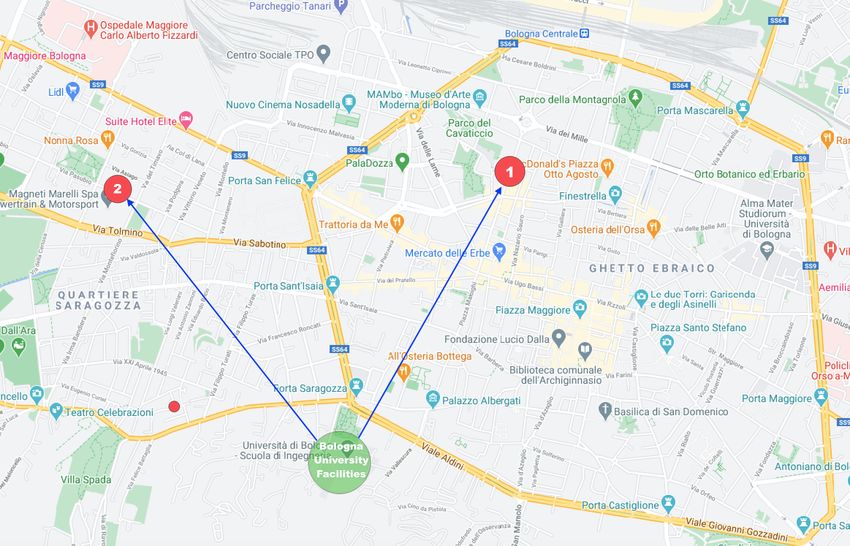
(a)                                            (b)                                               (c)
                Fig. 1: Distribution of the covered distances (a), the travel times (b) and the average travel speeds (c).

        Fig. 2: Number of trips aggregated by weekdays.                                Fig. 4: Seasonality of cycling mobility.

                                                                         weekdays bikes are heavily used, possibly either for home-to-
                                                                         work or home-to-study. This assumption is also confirmed in
                                                                         Figure 3 as we can see that the most of the trips during the
                                                                         working days were happening from 07:00 to 09:00 and from
                                                                         17:00 to 19:00, that is, mostly connected with the time people
                                                                         move for either work or study and returning in the evening.
                                                                            Figure 4 shows the number of trips spread over the six
                                                                         months. We can observe that the number of trips reached its
                                                                         peak during May (25%) and then it gradually dropped down,
                                                                         reaching its lowest level during August. In particular, there was
                                                                         a 40% drop in trips from July to August. In August, only 30%
                                                                         of May’s trips were done. This behaviour can be explained
 Fig. 3: Weekends vs weekdays: the start and end times of work           as during summer more, and more people start leaving the
             represent two peaks during the week.                        city for vacations, and the off-site students start going back to
                                                                         their hometowns. However, in September the number of trips
                                                                         started increasing again, with an increase of 28% compared to
   Figures 1a and 1b provide the distribution of the covered             the number of trips in August, possibly due to the return of
distances and travel times, showing a peak around 1600 meters            students and people from holidays.
and 720 seconds, respectively. This highlights a characteristic
of the bike usage in Bologna that 40% of the trips cover less            B. Spatial analysis
than 1.6 kilometers distance for 12-13 minutes of travel time.              In this section, we discuss the paths used by bike users and
Whereas, Figure 1c shows the histogram of the average travel             the possible attractive hubs of the city. Bologna’s historical city
speeds with a peak of around 3.8-4 meters per second, that               centre covers an area of 4.5Km2 , which is the red polygon
is, compatible with the speed usually reported in experimental           shown in Figure 5. The city has several characteristics that
literature [30], [31].                                                   can help to understand urban mobility. In particular, the train
   Figure 2 shows the trips aggregated by weekdays. The                  station is located north of the city (denoted using “T” letter
84% of total trips done during working days suggests that on             in light blue color in Figure 5) just outside the historic centre

                                                                    4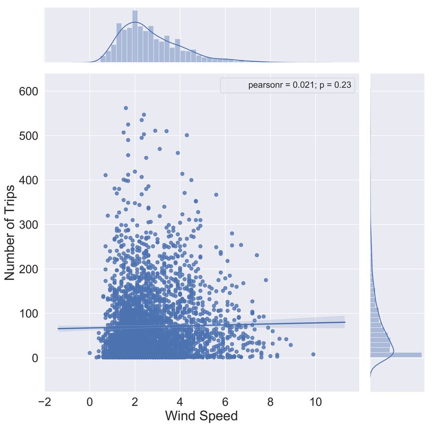
Fig. 5: Bologna Map.                  Fig. 6: Bike road network in May            Fig. 7: Bike road network in August

(denoted using “C” letter in purple color in Figure 5), and it is
one of the main nodes in the national railway network. Most
of the departments of the University of Bologna are distributed
within the historic centre, however, the engineering department
is located on the south west part of the city (denoted using “U”
letter in green color in Figure 5). There are two big hospitals
in the east and west of the city (denoted using “H” letter in
red color in Figure 5). During the day, there is a large number
of people who move to and from the city for work and study
purposes.
   1) Bike road network: In this section, we identify the road
                                                                                                    (a)
networks often used by the bike users (based on the dataset).
Figures 6 and 7 show which streets were the most used by bike
users through the density-based gradient palette for the months
of May 2017 and August 2017. For each month, we normalised
the data before plotting the graphs. The yellow roads were
the most used, while the red ones were used by a smaller
number of users. We can clearly observe the difference in
terms of bike usage between the two months. We can observe
that the density of the streets is similar, and the high-used paths
correspond to the main arteries of the centre’s road network.
The road network in Bologna has a radial structure and, since
the bicycle is used for medium-long trips, it is quite common
to cross the city passing through the centre.                                                       (b)
   2) Main hubs: The analysis of the trips allowed us to                  Fig. 8: Spreading out pattern from the Piazza Maggiore hub,
identify three main hubs of the city, which have a high                            difference between May (a) and August (b).
number of either start or end points. First being the Piazza
Maggiore – the main square and the neighborhood streets,
which are one of the main centers of city life. The other two                May is considered a “working month” and we can see
are the train station, and the engineering department of the                 that the main destinations were outside the city centre
University of Bologna. To understand how bike trips spread                   (Figure 8a). This indicates that most probably people
out from the three aforementioned hubs, we compared if there                 were going back to home after spending time in the
is a significant change in bike usage between the month of                   city centre (possibly from the workplaces and offices
May (chosen as one of the representatives of the non-holiday                 in the city center). Indeed, most of the trips ended in
period) and the month of August (holiday period) for each                    residential areas of the city. In contrast, during August,
hub. In Figures 8, 9, and 10, the locations were aggregated                  which is a “vacation month” most of the trips ended
by the number of trips started from the main hub (the green                  inside historical city centre (Figure 8b).
circles in each figure) and ended in the final destination (the           2) Similar to the findings of Zhao et al. [15], we find
ranked red dots in the figures). The circle size indicates the               out many people commute for work or studies and use
number of trips ending at that destination. In addition, we also             bikes to arrive at the train station or to ride from the
ranked these locations by inserting numbers in the circles.                  train station to their work or study place. In May, the
   1) The spreading pattern from Piazza Maggiore (in the city                four main destinations were various departments of the
       centre) changed considerably between May and August.                  university (Figure 9a), while in August (Figure 9b), the

                                                                      5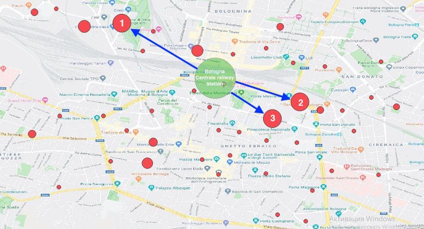
(a)
                              (a)

                              (b)
Fig. 9: Spreading out pattern from the train station hub, difference                                    (b)
                between May (a) and August (b).
                                                                            Fig. 10: Spreading out pattern from the engineering department
                                                                                   hub, difference between May (a) and August (b).
     final destinations changed and most of the trips ended
     in a large shopping mall just outside the city centre.                June to the end of August, when the average air temperature
  3) Considering the engineering department, it is inter-                  reaches 27 degrees or above, the number of trips starts to
     esting to note how the pattern changed from May to                    drop. In summary, we can confirm that bike trips are strongly
     August. During the month of May, when the lessons                     dependant on air temperature, which confirms the findings of
     are still in progress, a significant number of trips ended            many previous studies [6], [9].
     in places in the city where students spend their non-
     university time, such as student residences and pubs
     (Figure 10a). Whereas, for the month of August, the
     two most popular destinations turned out to be near to
     parks (Figure 10b). In addition, the number of trips also
     became very less in the month of August due to the
     holiday period.
C. Weather’s effects on bike usage
   In this section, we discuss the results about how weather
conditions, that is air temperature, precipitations and wind
speed, affect the number of bike trips during the six months
period.
   1) Air temperature: The spring in Bologna is characterized
by comfortable temperatures, while in the summer the weather
is hot and sultry. Comfortable weather conditions usually play
a significant role in bike usage, and when the air temperature              Fig. 11: Average daily air temperatures and the number of bike
is too high or too low, people prefer a different means of                                               trips.
transport [6]. Figure 11 shows the number of bike trips and
the trend of the temperature during the six months period.                   2) Precipitations: During the six months of the observation
Temperatures in April and May, which is around 20 degrees,                 period, most of the days were dry with no rain or snow.
is comfortable for making bike trips, while from mid of                    There were only some days from May 08 to May 14 and

                                                                       6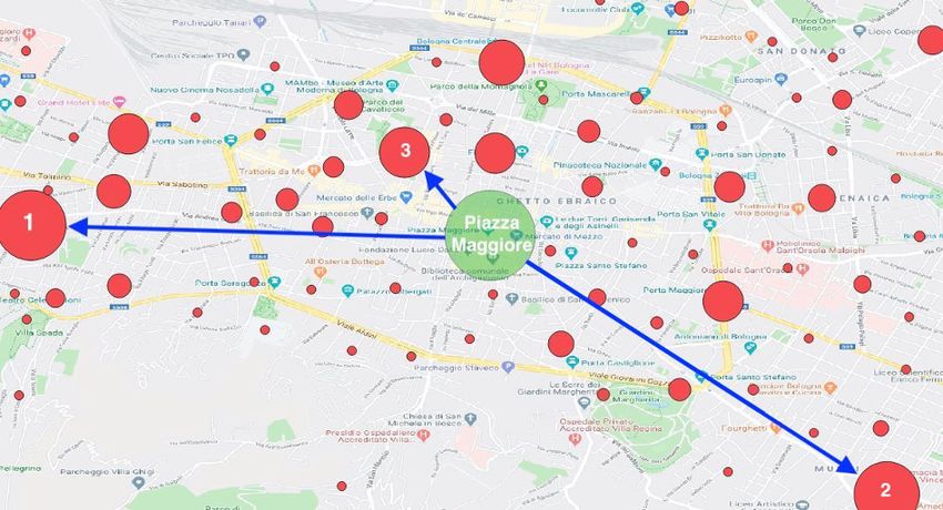
from September 04 to September 10 with some amount of                    raining from 8 pm to 10 pm, while on Sunday due to rain,
precipitations, while during other months, the number of rainy           which occurred from 2 am to 11 am, it led to a half number
days were significantly low. Thus, we decided to look into the           of trips.
weeks with the highest number of precipitations and compare                 3) Wind speed: Finally, we analysed how the speed of wind
them with the following week. In particular, we compared the             affects the bike usage. Figure 14 shows the number of trips
week from May 08 to May 14 against the week from May 15                  and the average wind speed during the six months period. The
to May 21 (Figure 12), and the week from September 04 to                 results show that there is no correlation between wind speed
September 10 against the week September 11 to September                  and number of bike trips during the observation period.
17 (Figure 13).

Fig. 12: Precipitation amount and number of trips during different
                          weeks in May.

   From May 08 to May 14, there were two rainy days, that is
Tuesday and Friday, and they heavily affected the number of
bike trips (Figure 12). In particular, on Tuesday the number of
trips were less than half compared the next week’s Tuesday.
However, there was a small difference between the number of
trips during Fridays. It is to be noted that most of the trips
were made in the early morning hours, as shown in Figure 3.                  Fig. 14: Average wind speed and the number of bike trips.
Looking into hourly data, we detected that on May 09, there
were heavy rains from 2 am to 9 am that strongly affected
the number of trips, while on May 12, it was raining only for            D. Pollution and bike usage
one hour around 3 pm, and this did not significantly affect the             Being one of the most ecological means of transportation,
number of trips.                                                         there is a notion that the usage of bikes might decrease
                                                                         the pollution of air [32], [33]. We analysed the changes in
                                                                         four different indicators of air pollution during the period
                                                                         of observation, that is i) Particulate matter (PM), ii) Ozone
                                                                         (O3), iii) Nitrogen dioxide (NO2), and iv) Sulfur dioxide
                                                                         (SO2). However, no positive or negative correlation could be
                                                                         identified. We also analysed if there were any changes in the
                                                                         indicators for separate streets that were being heavily used by
                                                                         bicycles. Similarly, we could not find any correlation between
                                                                         air pollution and bike use during the period of observation.
                                                                         Possibly reasons for this result could be due to having a low
                                                                         amount of observations about air pollution and the lack of car
                                                                         usage data.
Fig. 13: Precipitation amount and number of trips during different
                                                                         E. Holidays and events
                        weeks in September.
                                                                            In this last section, we discuss how holidays, events, such
The same goes for the comparison between the two weeks of                as protests and strikes, and national celebration affect the bike
September (Figure 13). In particular, from September 04 to               usage. During the period of observation, there were 14 public
September 10, there were two rainy days, that is Saturday and            holidays. Figure 15 shows the bike trips aggregated by day of
Sunday. On Saturday, the number of trips remained unchanged              the week for April (Figure 15a) and September (Figure 15b),
compared to the Saturday of the following week since it was              where the changes in the bike usage were more evident. In

                                                                     7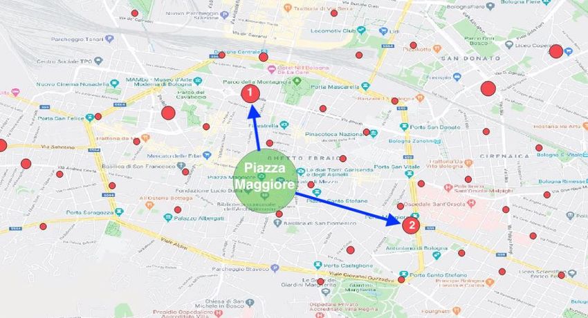
V. P REDICTIVE A NALYSIS
                                                                          In this section, we present the results of the predictive
                                                                        analysis with the aim to predict bike trips for the next 30
                                                                        and 60-minutes.

                                                                        A. Predictive algorithms and Metrics:
                                                                          We employed various methods, that is Linear Regression,
                                                                        Random Forest, Extreme Gradient Boosting (XGBoost), and
                                                                        LSTM for the predictive task. The prediction models are
                                                                        evaluated using different metrics that allow understanding the
                                (a)                                     performance of the predictive algorithms. In particular, given
                                                                        the regression nature of the prediction, we used the following
                                                                        metrics: Mean Absolute Error (MAE), Mean Squared Error
                                                                        (MSE), Root Mean Squared Error (RMSE), and R2 metrics.

                                                                        B. Feature selection
                                                                           We manually selected the features for the prediction. In par-
                                                                        ticular, we selected the following features: temperature, pre-
                                                                        cipitation, hour_of_the_day, month, season (spring, summer
                                                                        and autumn), day_of_week (Monday, Tuesday, ..., Sunday),
                                                                        holiday (whether a day is a holiday or not), hour_history, and
                                                                        week_history. The last two variables represent the number of
                                                                        trips for one hour and one week before, respectively. Based on
                                (b)
                                                                        the results shown in Sections IV-C3 and IV-D, we excluded
 Fig. 15: Number of bike trips aggregated by day of the week for
each week, for April (a) and August (b). Holidays are marked with
                                                                        wind speed and air pollution in our final evaluation.
                            a blue star.
                                                                        C. Experimental setup
                                                                           In order to predict bike usage in the next 30 and 60-minutes,
particular, the results show a significant difference during the        we have prepared two datasets. In the first one, we aggregated
Easter holidays (April 16-17, 2017) and during Ferragosto8              the number of trips by 30-minutes time slots, while in the
(i.e., August 15, 2017). Figure 15a shows that during Easter            second one, we aggregated the number of trips by hours. In
holidays, the number of trips dropped by 35% on Good Friday,            both datasets, we converted categorical variables into dummy
over by 50% on Holy Saturday and Easter Sunday, that is                 variables. We computed the correlation among all the variables
the orange bars in the figure, and almost by 80% on Easter              with the number of trips, and we found out that the number
Monday, that is the green bar in the figure. Figure 15b shows           of trips is mostly correlated with hour_history, week_history,
that during Ferragosto in August 2017, that is the green bar in         temperature, month, and season (i.e., spring, summer, and
the Figure, the number of trips dropped by 60% in comparison            autumn). In addition, we used four different splits that is,
to the number of trips done one week before and after.                  90/10, 80/20, 70/30, and 60/40 for training/test ratio. For each
                                                                        split, we applied the 10-fold Cross-Validation technique on the
   Next, we analysed how events such as protests, strikes, and
                                                                        training set and evaluate it on the test data.
large gatherings in the city affect the bike usage. The reason
behind analyzing the impact of these type of events is the              D. Prediction results
following: during protests or strikes, the number of main roads
                                                                           Among all the prediction models, LSTM gave the best
are being diverted, blocked, or closed, which may lead to an
                                                                        results9 . Table I provides the results for the next 60-minutes
increased number of bike trips that represents a more agile
                                                                        interval prediction for the 90/10 split. We can notice that the
means of transportation. On the other hand, a strike may also
                                                                        LSTM model is almost 4.5 times better than the others, and
decrease the usage of bikes as people may decide not to go
                                                                        the second-best model is the Random Forest, which is slightly
to work. Analyzing the protests in Bologna during the six
                                                                        better than Linear Regression and XGBoost. Thus, considering
months period, we did not notice any significant change in
                                                                        the best performance of the LSTM model, we provide results
the usage of the bike. It is worth mentioning that most of the
                                                                        with various data split ratios in Table II, both for the 60-
protests and strikes were not large and did not last for more
                                                                        minutes as well as for the 30-minutes interval prediction. The
than a few hours. Also, although no information was found
                                                                        best results were achieved with 90/10 split ratio. It is worth
on the closure of the roads, the number of bike trips did not
                                                                        to notice that the results improve significantly by reducing
significantly change during these events.
                                                                        the prediction interval (30-minutes). In particular, predicting
  8 Assumption   of Mary day.                                             9 We   are not showing all the results due to space limitation.

                                                                    8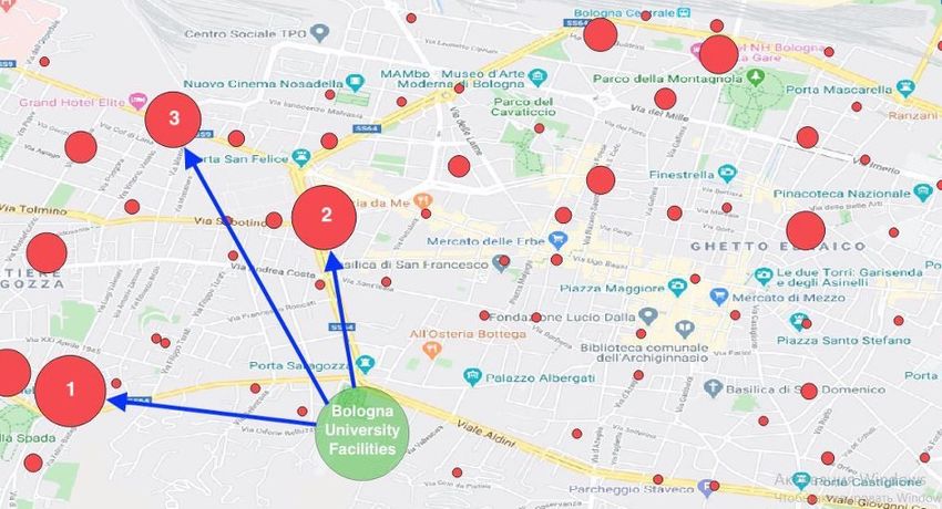
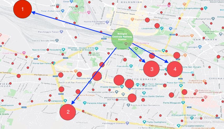
Fig. 16: LSTM model 30-minute prediction over the test set of 18-day (September 13, 2017 - September 30, 2017).

30-minutes interval improves the results on average 4 times                         In this paper, we presented a descriptive and predictive
in comparison with 60-minutes predictions. The importance                        analysis of bike usage for the city of Bologna. In particular,
of hour_history feature can be noted by that it improved the                     we analysed temporal and spatial patterns of bike users and
model on an average by 30%, considering MSE, MAE and                             the impact of weather conditions, such as air temperature,
RMSE results. Whereas the week_history feature improved                          precipitation, and wind speed, pollution conditions, and hol-
the results by around 45%. As a micro analysis, Figure 16                        idays on the bike usage. Moreover, we compared different
shows the LSTM prediction results over the 18 days of the                        models to predict the trips for the short-term period, that is,
test set (September 13, 2017 - September 30, 2017). Each                         30-minutes and 60-minutes time interval. The results show
time step on the graph is 30 minutes and it is worth noticing                    a seasonality of cycling trips and more in detail a weekly
that the prediction trend (i.e., the red line in the graph) almost               trend in favour of working days, which is congruent with a
completely overlaps the observation trend (i.e., the blue line                   commuting behaviour from/to work and study place. Also, the
in the graph).                                                                   spatial analysis confirms this result, in particular, we found
                                                                                 several attractive points that coincide with places of study,
                   Method     MAE       MSE     RMSE       R2                    which were less frequently visited during the summer period.
          Linear Regression   46.03   4438.29   66.62     0.25
             Random Forest    44.72   4354.25   65.98     0.33                   The several supplementary datasets used in the descriptive
                  XGBoost     47.04   4809.13   69.34     0.17                   analysis allowed to confirm a negative correlation between
                    LSTM      16.62    457.73   21.39     0.91                   bike trips and precipitation and highlight that temperature
 TABLE I: Models comparison in 60-minutes interval prediction                    around 26/27 degrees and over leads to a decrease in the
                  using 90/10 split ratio.                                       number of bike trips. However, we did not find evidence
                                                                                 about the correlation between air pollution and bike usage.
  Split        MAE             MSE             RMSE              R2
                                                                                 In the predictive analysis, we found that LSTM provides
  ratio     60     30      60       30      60     30      60          30        the best results and that too for predicting for 30-minutes
  90/10    16.62  5.38   457.73    66.08   21.39  8.12    0.91        0.91       (compared to 60-minutes) time interval, which could be of
  80/20    23.62  6.42   986.56   104.54   31.40  10.22   0.63        0.86
  70/30    25.44  5.62   1140.87   70.63   32.45  8.40    0.70        0.87       practical help to management of traffic infrastructure (e.g.,
  60/40    16.75  6.03   546.67    98.64   23.38  9.13    0.75        0.85       traffic lights, temporary traffic detours) on road network links.
 TABLE II: Prediction results varying the split ratio. The values                Additionally, the model can be used to predict the demand
       represents the LSTM model results predicting                              gap for strengthening the bike-sharing services, which usually
        60-minutes/30-minutes interval, respectively.
                                                                                 require a redistributing service to make sure that people who
                                                                                 would like to use bikes will most certainly find one near their
                                                                                 location.
                         VI. C ONCLUSIONS
                                                                                    As future works, several directions can be considered.
   The significantly growing awareness about climate change                      Firstly, we plan to analyse the other transport data within the
and pollution has given rise to the need for eco-friendly and                    Bella Mossa dataset to understand interactions with bike usage
healthy means of transportation. Cycling allows lightening                       and different behaviour in the use of the city’s road network.
road traffic within touristic and historical cities where the                    We also plan to study a larger dataset with a longer timeline
traffic congestion is exacerbated. Thus, understanding cycling                   to improve analysis of seasonal factors that may also improve
mobility is of the utmost importance to improve bike infras-                     the prediction results. Finally, we plan to compare the patterns
tructures and encourage bike use.                                                of bike users from different cities.

                                                                             9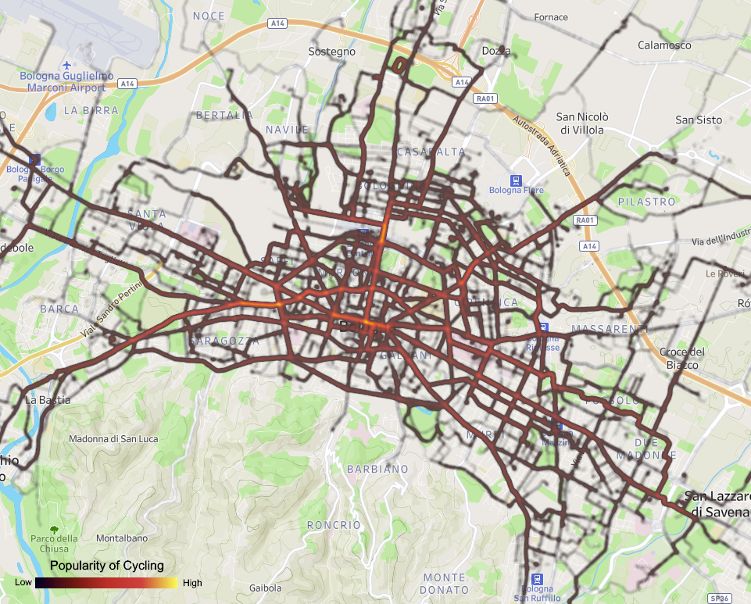
ACKNOWLEDGMENT                                                [19] J. Zhang, X. Pan, M. Li, and S. Y. Philip, “Bicycle-sharing system
                                                                                            analysis and trip prediction,” in 2016 17th IEEE international conference
   We are grateful to SRM Reti e Mobilità Srl for providing                                 on mobile data management (MDM), vol. 1. IEEE, 2016, pp. 174–179.
the data of the Bella Mossa program 2017. This research                                [20] Y. Ai, Z. Li, M. Gan, Y. Zhang, D. Yu, W. Chen, and Y. Ju, “A deep
                                                                                            learning approach on short-term spatiotemporal distribution forecasting
is financially supported by H2020 SoBigData++ and CHIST-                                    of dockless bike-sharing system,” Neural Computing and Applications,
ERA SAI project.                                                                            vol. 31, no. 5, pp. 1665–1677, 2019.
                                                                                       [21] C. Xu, J. Ji, and P. Liu, “The station-free sharing bike demand
                              R EFERENCES                                                   forecasting with a deep learning approach and large-scale datasets,”
                                                                                            Transportation research part C: emerging technologies, vol. 95, pp. 47–
 [1] C. Mizzi, A. Fabbri, S. Rambaldi, F. Bertini, N. Curti, S. Sinigardi,                  60, 2018.
     R. Luzi, G. Venturi, M. Davide, G. Muratore et al., “Unraveling                   [22] C. Zhang, L. Zhang, Y. Liu, and X. Yang, “Short-term prediction of bike-
     pedestrian mobility on a road network using icts data during great tourist             sharing usage considering public transport: A lstm approach,” in 2018
     events,” EPJ Data Science, vol. 7, no. 1, p. 44, 2018.                                 21st International Conference on Intelligent Transportation Systems
 [2] D. O. Rodrigues, A. Boukerche, T. H. Silva, A. A. Loureiro, and L. A.                  (ITSC). IEEE, 2018, pp. 1564–1571.
     Villas, “Combining taxi and social media data to explore urban mobility           [23] N. Duc-Nghiem, N. Hoang-Tung, A. Kojima, and H. Kubota, “Modeling
     issues,” Computer Communications, vol. 132, pp. 111–125, 2018.                         cyclists’ facility choice and its application in bike lane usage forecast-
 [3] R. Zhu, X. Zhang, D. Kondor, P. Santi, and C. Ratti, “Understanding                    ing,” IATSS research, vol. 42, no. 2, pp. 86–95, 2018.
     spatio-temporal heterogeneity of bike-sharing and scooter-sharing mo-             [24] D. Singhvi, S. Singhvi, P. I. Frazier, S. G. Henderson, E. O’Mahony,
     bility,” Computers, Environment and Urban Systems, vol. 81, p. 101483,                 D. B. Shmoys, and D. B. Woodard, “Predicting bike usage for new
     2020.                                                                                  york city’s bike sharing system,” in Workshops at the twenty-ninth AAAI
 [4] S. J. Mooney, K. Hosford, B. Howe, A. Yan, M. Winters, A. Bassok,                      conference on artificial intelligence, 2015.
     and J. A. Hirsch, “Freedom from the station: Spatial equity in access             [25] H. Luo, Z. Kou, F. Zhao, and H. Cai, “Comparative life cycle assess-
     to dockless bike share,” Journal of transport geography, vol. 74, pp.                  ment of station-based and dock-less bike sharing systems,” Resources,
     91–96, 2019.                                                                           Conservation and Recycling, vol. 146, pp. 180–189, 2019.
 [5] T. Liu, Z. Yang, Y. Zhao, C. Wu, Z. Zhou, and Y. Liu, “Temporal                   [26] G. McKenzie, “Docked vs. dockless bike-sharing: Contrasting spa-
     understanding of human mobility: A multi-time scale analysis,” PloS                    tiotemporal patterns (short paper),” in 10th international conference on
     one, vol. 13, no. 11, p. e0207697, 2018.                                               geographic information science (giscience 2018). Schloss Dagstuhl-
 [6] T. Nosal and L. F. Miranda-Moreno, “The effect of weather on the use of                Leibniz-Zentrum fuer Informatik, 2018.
     north american bicycle facilities: A multi-city analysis using automatic          [27] S. Shaheen and A. Cohen, “Shared micromoblity policy toolkit: Docked
     counts,” Transportation research part A: policy and practice, vol. 66,                 and dockless bike and scooter sharing,” 2019.
     pp. 213–225, 2014.                                                                [28] T. Gu, I. Kim, and G. Currie, “To be or not to be dockless: Empirical
 [7] B. Caulfield, M. O’Mahony, W. Brazil, and P. Weldon, “Examining                        analysis of dockless bikeshare development in china,” Transportation
     usage patterns of a bike-sharing scheme in a medium sized city,”                       Research Part A: Policy and Practice, vol. 119, pp. 122–147, 2019.
     Transportation research part A: policy and practice, vol. 100, pp. 152–           [29] Y. Shen, X. Zhang, and J. Zhao, “Understanding the usage of dockless
     161, 2017.                                                                             bike sharing in singapore,” International Journal of Sustainable Trans-
 [8] W. El-Assi, M. S. Mahmoud, and K. N. Habib, “Effects of built                          portation, vol. 12, no. 9, pp. 686–700, 2018.
     environment and weather on bike sharing demand: a station level                   [30] M. Dozza and J. Werneke, “Introducing naturalistic cycling data: What
     analysis of commercial bike sharing in toronto,” Transportation, vol. 44,              factors influence bicyclists’ safety in the real world?” Transportation
     no. 3, pp. 589–613, 2017.                                                              research part F: traffic psychology and behaviour, vol. 24, pp. 83–91,
 [9] M. Nankervis, “The effect of weather and climate on bicycle commut-                    2014.
     ing,” Transportation Research Part A: Policy and Practice, vol. 33, no. 6,        [31] G. Menghini, N. Carrasco, N. Schüssler, and K. W. Axhausen, “Route
     pp. 417–431, 1999.                                                                     choice of cyclists in zurich,” Transportation research part A: policy and
[10] J. Sears, B. S. Flynn, L. Aultman-Hall, and G. S. Dana, “To bike or                    practice, vol. 44, no. 9, pp. 754–765, 2010.
     not to bike: Seasonal factors for bicycle commuting,” Transportation              [32] O. Hertel, M. Hvidberg, M. Ketzel, L. Storm, and L. Stausgaard, “A
     research record, vol. 2314, no. 1, pp. 105–111, 2012.                                  proper choice of route significantly reduces air pollution exposure - a
[11] E. Fishman, S. Washington, N. Haworth, and A. Watson, “Factors                         study on bicycle and bus trips in urban streets,” Science of the total
     influencing bike share membership: An analysis of melbourne and                        environment, vol. 389, no. 1, pp. 58–70, 2008.
     brisbane,” Transportation research part A: policy and practice, vol. 71,          [33] C. Johansson, B. Lövenheim, P. Schantz, L. Wahlgren, P. Almström,
     pp. 17–30, 2015.                                                                       A. Markstedt, M. Strömgren, B. Forsberg, and J. N. Sommar, “Impacts
[12] D. Fuller, L. Gauvin, Y. Kestens, M. Daniel, M. Fournier, P. Morency,                  on air pollution and health by changing commuting from car to bicycle,”
     and L. Drouin, “Use of a new public bicycle share program in montreal,                 Science of the total environment, vol. 584, pp. 55–63, 2017.
     canada,” American journal of preventive medicine, vol. 41, no. 1, pp.
     80–83, 2011.
[13] J. Molina-García, I. Castillo, A. Queralt, and J. F. Sallis, “Bicycling
     to university: evaluation of a bicycle-sharing program in spain,” Health
     promotion international, vol. 30, no. 2, pp. 350–358, 2015.
[14] J. E. Froehlich, J. Neumann, and N. Oliver, “Sensing and predicting the
     pulse of the city through shared bicycling,” in Twenty-First International
     Joint Conference on Artificial Intelligence, 2009.
[15] J. Zhao, J. Wang, and W. Deng, “Exploring bikesharing travel time and
     trip chain by gender and day of the week,” Transportation Research Part
     C: Emerging Technologies, vol. 58, pp. 251–264, 2015.
[16] P. Borgnat, P. Abry, P. Flandrin, C. Robardet, J.-B. Rouquier, and
     E. Fleury, “Shared bicycles in a city: A signal processing and data
     analysis perspective,” Advances in Complex Systems, vol. 14, no. 03,
     pp. 415–438, 2011.
[17] H. Xu, J. Ying, H. Wu, and F. Lin, “Public bicycle traffic flow prediction
     based on a hybrid model,” Applied Mathematics & Information Sciences,
     vol. 7, no. 2, p. 667, 2013.
[18] Y. Li, Y. Zheng, H. Zhang, and L. Chen, “Traffic prediction in a bike-
     sharing system,” in Proceedings of the 23rd SIGSPATIAL International
     Conference on Advances in Geographic Information Systems, 2015, pp.
     1–10.

                                                                                  10
You can also read