Improving weather forecasting by assimilation of water vapor isotopes
←
→
Page content transcription
If your browser does not render page correctly, please read the page content below
www.nature.com/scientificreports
OPEN Improving weather forecasting
by assimilation of water vapor
isotopes
Masataka Tada1, Kei Yoshimura2* & Kinya Toride2,3
Stable water isotopes, which depend on meteorology and terrain, are important indicators of global
water circulation. During the past 10 years, major advances have been made in general circulation
models that include water isotopes, and the understanding of water isotopes has greatly progressed
as a result of innovative, improved observation techniques. However, no previous studies have
combined modeled and observed isotopes using data assimilation, nor have they investigated the
impacts of real observations of isotopes. This is the first study to assimilate real satellite observations
of isotopes using a general circulation model, then investigate the impacts on global dynamics and
local phenomena. The results showed that assimilating isotope data improved not only the water
isotope field but also meteorological variables such as air temperature and wind speed. Furthermore,
the forecast skills of these variables were improved by a few percent, compared with a model that did
not assimilate isotope observations.
Extreme weather is associated with natural disasters, and it impacts energy consumption and economics1.
Improvements in weather forecasting can help mitigate the impact of climate change on global water resources,
which is projected to i ncrease2–4. In this study, the impacts of water vapor isotopes on weather forecasting were
investigated using satellite observations. These isotopes are used as tracers to study the Earth’s water circulation
in hydrology, meteorology, and climatology a pplications5–7.
Water vapor isotopes are sensitive to phase transition, and heavier molecules such as H2HO or H 218O pref-
erentially condense/less preferentially evaporate, compared with ordinary H 2O. The spatiotemporal variability
of isotopes depends on these characteristics. This unique behavior is called the stable isotope effect, which was
formulated empirically by Dansgaard8. Dansgaard found that the geographic distribution of isotopes in precipita-
tion is related to latitude, air temperature, altitude, precipitation, and distance from the coast.
These unique characteristics have been noted, and observations have been collected for geoscientific research
since 19619–11 in the Global Network of Isotopes in Precipitation (GNIP) by the International Atomic Energy
Agency (IAEA). However, the GNIP has only several hundred stations worldwide and observes isotopes in
surface precipitation, which holds integrated information about various atmospheric processes. These data are
both spatially and temporally much sparser than conventional non-isotopic data (e.g., wind, air temperature, and
pressure). Recently, the performance of satellite-based spectrometers and the algorithms used to retrieve isotopes
in atmospheric water vapor have both been improved12–15, and the improved versions are more directly sensitive
to atmospheric processes. Previous studies indicated that δ2H observations provide an understanding of moisture
processes due to isotopic fractionation16–19. Such studies include the estimation of condensation efficiency in
convective activity12,16, the transport processes of dry air masses in the Sahel13, constraining vertical water vapor
transport to reduce the moisture bias of models in the mid and upper troposphere17,18, and investigations of the
hydrological cycle associated with large-scale convective r eorganization19.
In parallel with enhancements in observation technology, numerical models that incorporate water isotopes
have been developed and i mproved20–30. These models calculate the distribution of isotopes and provide infor-
mation on the circulation of water isotopes in the absence of observations. Using an isotope-enabled numerical
model, a past study investigated the impacts of assimilating water isotopes in idealized e xperiments31. Although
the results indicated that atmospheric fields can be improved by assimilating water vapor isotopes, satellite-based
observations such as those from the Tropospheric Emission Spectrometer (TES) and the Scanning Imaging
1
Japan Weather Association, 55F Sunshine City 60, Higashiikebukuro 3‑1‑1, Toshima‑ku, Tokyo 170‑6055,
Japan. 2Institute of Industrial Science, The University of Tokyo, 5‑1‑5, Kashiwanoha, Kashiwa‑shi, Chiba 277‑8574,
Japan. 3Department of Atmospheric Sciences, University of Washington, Seattle, WA 98195, USA. *email: kei@
iis.u-tokyo.ac.jp
Scientific Reports | (2021) 11:18067 | https://doi.org/10.1038/s41598-021-97476-0 1
Vol.:(0123456789)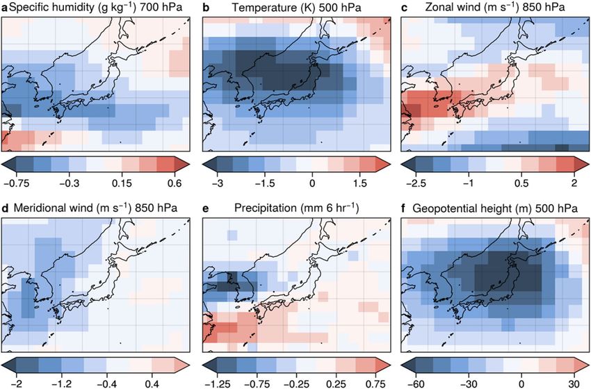
www.nature.com/scientificreports/
Absorption Spectrometer for Atmospheric Cartography (SCIAMACHY) had less robust impacts than did mock
in situ observations because of differences in the number of observations.
In this study, we investigated the utility of water vapor isotope data derived from the Infrared Atmospheric
Sounding Interferometer (IASI)14, which has a much greater spatial and temporal observation coverage with
improved accuracy, compared with TES and SCIAMACHY. IASI observes water vapor isotopes in the mid-
troposphere globally twice per day. We evaluated the impact of assimilating IASI isotope data on various atmos-
pheric fields and forecast accuracy.
Methodology
Assimilation scheme. We used a local ensemble transform Kalman filter (LETKF) for our data assimi-
lation scheme. The Kalman filter (KF) estimates optimal values using a linear minimum variance estimation
considering the covariance in both observation and model errors. The LETKF has a high calculation efficiency
because of the localization technique32. The model error covariance is assumed to be represented by the covari-
ance of a limited number of ensemble members. In our study, we used 30 ensemble members.
The analysis field, xa , a matrix that serves as the initial conditions, is calculated by a linear combination of
first guess and observation values as follows:
xa = xf + K y◦ − H xf , (1)
where xa consists of all prognostic variables of the model (zonal and meridional wind speed, air temperature,
specific humidity, surface pressure, and hydrogen isotope ratio) at all model grids (192 × 94 × 28) for all 30
ensemble members; xf is the first guess (i.e., the forecasted field from the analysis of the previous cycle; 6 h ago
in our study); K is the Kalman gain; y° is the IASI observation; and H is the observation operator that projects the
Isotope-incorporated Global Spectral Model (IsoGSM) model field to the IASI observations field. Here, H is the
spatial interpolation from the IsoGSM grids to the locations of IASI observations. The satellite averaging kernels
were not applied to the model output in this study. The second term on the right side is the analysis increment,
which indicates the degree of modification from the first guess.
Observation data. We used IASI data for the data assimilation. Although our IASI data had 10 vertical
layers, we assimilated only the fifth layer (at the height of approximately 4.5 km from the surface) because it con-
tained the most reliable δ2H measurements14. Horizontal spatial coverage of IASI δ2H observations is from 60°
S to 60° N. IASI makes approximately 1.3 million measurements per day, but only cloud-free measurements can
be used to retrieve δ2H estimates. After removing obvious outliers and resampling to model resolution, nearly
230,000 points for April 2013 were used in the assimilation. The spatial distribution of δ2H observation points
and monthly averaged data are shown in Fig. S1.
Numerical model. We used IsoGSM as our numerical model with T62 horizontal resolution (approxi-
mately 200 km) and 28 vertical sigma levels25. Gaseous forms of heavier isotopologues ( H2HO and H 218O) are
incorporated into IsoGSM as prognostic variables, in addition to ordinary water vapor. All water isotopes are
advected and transported by atmospheric circulation processes and subgrid-scale processes (convection and
boundary layer turbulence). In addition, the fractionation during phase transitions, such as condensation or
evaporation of precipitation, is also formulated in detail. The model’s physics packages include the longwave and
shortwave radiation scheme of Chou and S uarez33, relaxed Arakawa–Schubert convective p arameterization34,
nonlocal vertical diffusion35, mountain drag36, shallow convection37, and the Noah land surface scheme38.
IsoGSM has been widely used in previous s tudies39. For example, IsoGSM was used to reproduce spatiotem-
poral variation in the isotopic field for the past 30 y ears25 by nudging with data from the National Centers for
Environmental Prediction/Department of Energy (NCEP/DOE) r eanalysis40. We used this dataset (referred to
as isotopic reanalysis) to validate the assimilation experiments in this study because it has comparable accuracy
to that of the NCEP/DOE reanalysis in terms of synoptic-scale fluctuation. The IsoGSM is one of few available
isotopic reanalyses, and has been well validated with satellite measurements of water vapor isotopes41.
Experimental setup. Our first experiment was conducted from 1 April to 6 May 2013 because of IASI data
availability. The last 6 days (i.e., 1–6 May 2013) were considered the pure forecast period. Our second experi-
ment was from 1–28 April 2013, and 23–28 April was used as the pure forecast period (Fig. S2). The calculation
process is shown in Fig. S3. First, we generated 30 ensemble members with perturbed initial conditions using
the lagged average forecast method42. Second, we made first-guess ensemble forecasts using IsoGSM. Third, we
estimated the analysis fields based on the first guess and observations using the LETKF. Finally, we repeated the
second and third processes. Note that IsoGSM and the LETKF are independent. IsoGSM simulated the mixing
ratios of H2HO in the air (hereafter qH2HO) as a prognostic variable, and we converted these ratios to the isotope
ratio of water vapor (hereafter δ2H) before the assimilation process as shown in Figure S3. This approach was
used because mixing ratios have a lower bound of zero, which often violates the Gaussian assumption in LETKF.
This conversion has also been employed in previous studies39,43. We decided to use 30 ensemble members, given
the results of idealized experiments (data not shown).
Importantly, our non-assimilation experiment was a set of realizations of the atmosphere initialized from
different dates in the natural run. Therefore, we considered the non-assimilation experiment to be independent
of the truth; we considered the ensemble average of the non-assimilation experiment to be closer to a climato-
logical condition.
Scientific Reports | (2021) 11:18067 | https://doi.org/10.1038/s41598-021-97476-0 2
Vol:.(1234567890)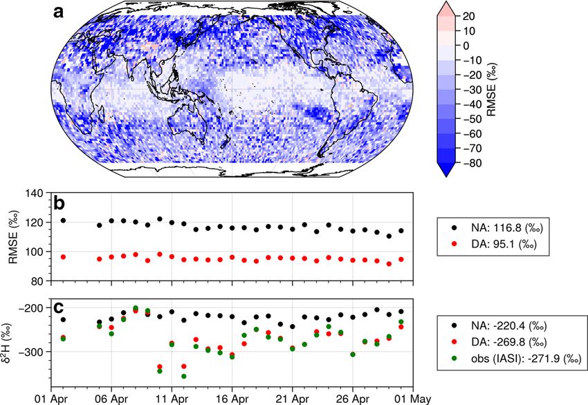
www.nature.com/scientificreports/
Figure 1. (a) Difference in root mean square error (RMSE) of 6-hourly δ2H in April for assimilation and non-
assimilation experiments. Blue (red) indicates better (worse) performance when assimilating water isotopes.
(b) 6-hourly time series of globally averaged RMSE of δ2H using IASI observation data from April 2013 at the
assimilation altitude of approximately 4.5 km. (c) Time series of δ2H over Japan and the surrounding area where
analysis skill was substantially improved for the middle troposphere. Black points indicate non-assimilation
experiment, red points indicate assimilation experiment, and green points indicate IASI observations. Black and
red points are collocated averages of IASI observations. Figure created using Python 3.7.6 (https://www.python.
org/).
In this study, we evaluated the accuracy of the analysis/forecast field based on changes in root mean square
errors (RMSEs) between the assimilation and non-assimilation experiments. Specifically, we used the analy-
sis/forecast skill defined by the difference between RMSEDA/FC and RMSENA, or the difference normalized by
RMSENA, defined as:
RMSEDA/FC − RMSENA
Analysis/forecst skill = × 100, (2)
RMSENA
where RMSEDA/FC is the RMSE of the analysis/forecast field against reanalysis data (isotopic reanalysis25 or
ERA544), and RMSENA is the RMSE of the non-assimilation experiment. Negative values indicate a higher accu-
racy than the non-assimilation experiment.
Results and discussion
The global impact of assimilating water vapor isotopes. We conducted experiments with and with-
out assimilating IASI data for 1–30 April 2013. Figure 1 shows the impacts of assimilating water vapor isotopes.
The analysis skill improved, especially in mid-latitudes (Fig. 1a) due to the high number of observations. Simi-
larly, a greater improvement was observed in the Northern Hemisphere than in the Southern Hemisphere. This
was because of the difference in available observations and the accuracy of observed hydrogen isotopes. A previ-
ous study found larger observational errors at middle and high latitudes in the winter h emisphere45.
However, improvements were limited at low latitudes, although many observations were assimilated (Fig. S1a).
This was probably because of the poor consistency between modeled and observed isotopic behavior at low lati-
tudes due to the poor representation of the latitude effect associated with the convective process, as demonstrated
by a previous study comparing modeled isotopes with TES and SCIAMACHY d ata41.
Figure 1b shows 6-hourly time series of globally averaged RMSE of δ2H using IASI observation from April
2013 at the assimilation altitude of approximately 4.5 km. During the study period, the isotope assimilation
improved RMSE by at least 10% globally. We further investigated how assimilating water vapor affected other
variables on a global scale. Figure S4 shows the vertical profile of the normalized change in RMSEs between the
two experiments, using the isotopic reanalysis as a reference. Although assimilating water isotopes improved
most variables globally throughout most of the troposphere, the profile of improved skills differed among vari-
ables. Furthermore, we compared the results with an ERA5 reanalysis (i.e., the ECMWF atmospheric reanalysis
in Fig. S5). The results indicated almost the same behavior as in the isotopic reanalysis, confirming the positive
effects of isotope assimilation on various atmospheric fields. Notably, the ERA5 data were spatially interpolated
to match the resolution of IsoGSM.
Scientific Reports | (2021) 11:18067 | https://doi.org/10.1038/s41598-021-97476-0 3
Vol.:(0123456789)www.nature.com/scientificreports/
Figure 2. Difference in RMSEs between assimilation and non-assimilation experiments during April 2013
over Japan for (a) specific humidity, (b) temperature, (c) zonal wind, (d) meridional wind, (e) precipitation
rate, and (f) geopotential height. The RMSE is derived from a 6-hourly time series with the isotopic reanalysis
as a reference. Blue is better, red is worse (for the assimilation experiment). If the number is negative, the
assimilation experiment was better than the non-assimilation experiment. Figure created using Python 3.7.6
(https://www.python.org/).
Specific humidity and air temperature were improved at the assimilation altitude (4.5 km), because these
variables are directly related to water vapor isotopes through isotopic fractionation. The analysis skills for geo-
potential height, zonal wind speed, and meridional wind speed were not necessarily improved at 4.5 km altitude,
but they were improved overall for the rest of the troposphere. This was because variables not directly related
to isotopes are indirectly improved by other variables directly related to isotopes, such as air temperature. Thus,
water isotopes hold integral information about the complex water cycle and the dynamics of moisture transport.
Local impacts of assimilating water vapor isotopes. Figure 1c shows the time series of regionally
averaged δ2H for Japan and the surrounding area, a region where analysis skill was particularly improved for
the mid-troposphere (Fig. 1a). In spring, the weather in Japan tends to change substantially due to the alter-
nate passage of low-pressure systems and traveling high-pressure s ystems46. Assimilating water vapor isotopes
helped represent these changes due to the abundant observations of water vapor isotopes in and upwind of
Japan (Fig. S1a). The analysis skill was not necessarily improved at points with a large number of observations
(Fig. S6a) because of the compound impacts of data assimilation and local meteorology (advection and convec-
tion).
Figure 2 shows the difference in RMSE derived from 6-hourly time series between assimilation and non-
assimilation experiments using the isotopic reanalysis over Japan. Assimilating water isotopes had positive effects
on specific humidity, air temperature, and winds (Fig. 2a–d,f) because water isotopes are sensitive to these vari-
ables. In contrast, the precipitation rate showed a deterioration for the domain average.
Specific humidity was improved over Japan and on the west side of Japan, whereas it worsened on the south
and north sides (Fig. 2a). The zonal wind worsened over Japan and on the west side of the country, contrary to
the specific humidity; it improved on the south and north sides of Japan. (Fig. 2c). The zonal wind was improved
over a large part of this area, but it deteriorated slightly over the eastern seas of Japan (Fig. 2d). Because water
vapor isotopes are inherently sensitive to precipitation processes, the precipitation-rate was improved to the
north of the domain, where the numbers of observations were large (Fig. 2e). Assimilating water vapor isotopes
generally had a positive impact in rainy regions such as from western China to the north of Japan, the sea to the
north of Australia, from the Bay of Bengal to the south of the Philippine Sea, and the sea to the east of the North
American continent (not shown). In contrast, geopotential height at 500 hPa may not have a direct relationship
Scientific Reports | (2021) 11:18067 | https://doi.org/10.1038/s41598-021-97476-0 4
Vol:.(1234567890)www.nature.com/scientificreports/
with isotopes; however, because of the close relationship with air temperature, improving the isotopic field
resulted in an improvement in geopotential height. We also made the same comparison using ERA5 (Fig. S7).
Overall, the results were similar to the findings of the isotopic reanalysis. This indicated the robustness of our
results, regardless of the choice of reanalysis datasets.
Focus on a low‑pressure event over Japan and the surrounding area. Here, we investigated a case
study of a low-pressure event over Japan on 19 April 2013 associated with precipitation. Considering the resolu-
tion of the model and the characteristics of the isotope effect, we chose a large-scale event to evaluate the impacts
of assimilating water isotopes, rather than a small and short phenomenon (e.g., a convective disturbance). As
explained in Sect. 2.4, the non-assimilation experiment was a set of free ensemble forecasts starting from differ-
ent initial conditions, such that the performance was closer to a climatological condition and it could not capture
any particular events by definition.
The left column of Fig. 3 shows the isotopic reanalysis fields, in which two low-pressure centers were observed
over eastern Japan (locations marked with white stars in Fig. 3a). We defined the centers of these low-pressure
systems using mean sea-level pressure and wind circulation: northern low near 42°N and 150°E, and southern
low near 32°N and 147°E. Corresponding to the low-pressure centers, a thermal trough was located over Japan
(Fig. 3b), and downward (upward motion) existed to the west (east) of the thermal trough (Fig. 3c). As expected,
rainfall occurred near the northern and southern lows (Fig. 3d), and winds at 500 hPa height blew along isobars
while surface winds indicated cyclonic circulation near the low-pressure centers.
The experiment with no isotope assimilation did not model the two low-pressure centers; however, the
experiment that assimilated the water vapor isotopes was able to simulate the northern low pressure (Fig. 3a).
The southern low pressure was not modeled as clearly, but a lower pressure area could be observed in the south
of Japan, which indicates that assimilating water vapor isotopes helped to produce the overall pressure structure
for the region. The difference in the ability to model the northern and southern lows indicates weak assimilation
constraints by the isotopes alone. However, the ability to model the overall pressure pattern simply by incorpo-
rating water vapor isotopes in the assimilation suggests the high potential of providing additional constraints
when combined with conventional observations. This possibility was demonstrated in recent research, with
idealization experiments assimilating traditional meteorological measurements42. Furthermore, the pressure field
in the assimilation experiment was more similar to the isotopic reanalysis in terms of high pressure to the west.
As explained in Sect. 3.2, the improvements in geopotential height were likely associated with improvements in
air temperature because of the strong relationship between isotopes and temperature.
The thermal trough was completely absent in the non-assimilation experiment, but in the assimilation experi-
ment, a weak trough was produced at a similar location as in the isotopic reanalysis (Fig. 3b). Vertical velocity was
completely different in the non-assimilation experiment and the isotopic reanalysis. The assimilation experiment,
however, was more accurate in terms of descending air occurring ahead of the low pressure and ascending air
occurring near the center of the low pressure (Fig. 3c).
In the non-assimilation experiment, precipitation occurred in regions not corresponding to the low-pressure
centers; in the assimilation experiment, precipitation occurred over the areas corresponding to the lows (Fig. 3d).
The assimilation grid in this region is shown in Fig. S6b. Although only the results over Japan are mentioned
here, precipitation was improved over Japan and across many regions on a global scale, as discussed in Sect. 3.2.
The wind field generally resembles the field of geopotential height because the wind blows along isobars at a
synoptic scale. At the 500-hPa level, the westerly wind blew zonally in the non-assimilation experiment, but it
blew along the analyzed thermal trough in the assimilation experiment. There was no cyclonic circulation in the
non-assimilation experiment near the surface, but circulation corresponding to the northern low was evident in
the assimilation experiment (Figs. 3a and d).
Model bias and model characteristics could not be completely eliminated, but we found that isotope infor-
mation overall improved synoptic-scale pressure patterns and other fields such as temperature, wind, and
precipitation.
Sensitivity to assimilation period. We conducted two 6-day forecast experiments to evaluate whether
water vapor isotopes can improve atmospheric forecasts. Assimilating water vapor isotopes improved many vari-
ables throughout the troposphere during the analysis period. We conducted these two experiments to investigate
how much forecast skill changes for different assimilation periods. We compared the forecast after 30 days of
assimilation with the forecast after 22 days of assimilation.
Figure 4 shows a comparison of the two assimilation experiments in terms of forecast skill against the non-
assimilation experiment. The blue bar indicates the assimilation experiment with a forecast period of 1–6 May
2013. The yellow bar indicates the assimilation experiment with a forecast period of 23–28 April 2013. Although
the assimilation periods and the prediction times differed, the assimilation forecast skill was better than the
non-assimilation forecast skill for many variables. In particular, air temperature forecast skill was improved by
approximately 3.5% in both forecast experiments (Fig. 4b). Furthermore, more improvements were obtained
with assimilation for 30 days than with assimilation for 22 days, in particular for precipitation and zonal wind
(Fig. 4a, c–f). As previous studies indicated, a longer assimilation period was closer to the truth during the spin-
up period45. Our results demonstrated that the accumulation of isotope observations helps improve weather
forecasting.
Scientific Reports | (2021) 11:18067 | https://doi.org/10.1038/s41598-021-97476-0 5
Vol.:(0123456789)www.nature.com/scientificreports/
Figure 3. Snapshot of a low-pressure system case study for Japan and the surrounding area on 19 April 2013 at
00:00 UTC for (a) 500 hPa pressure reduced to mean sea level (MSL; the two white stars indicate the locations
of the two low-pressure centers), (b) 500 hPa geopotential height, (c) vertical velocity at a height of 500 hPa,
and (d) precipitation rate. The orientation and length of the arrows indicate wind direction and speed (m s -1),
respectively. The number below the arrow in the legend for each panel indicates the wind speed for that arrow
length. Figure created using Python 3.7.6 (https://www.python.org/).
Scientific Reports | (2021) 11:18067 | https://doi.org/10.1038/s41598-021-97476-0 6
Vol:.(1234567890)www.nature.com/scientificreports/
Figure 4. Comparison of the two assimilation experiments on improvement in forecast skill over the non-
assimilation experiment for (a) precipitation rate, (b) 2-m temperature, (c) 10-m zonal wind, (d) 500-hPa
vorticity, (e) 700-hPa specific humidity, and (f) 600-hPa H2HO specific humidity. Forecast skill is defined as
the normalized difference in global RMSEs between assimilation and non-assimilation experiments during the
forecast period. Blue bar indicates the assimilation experiment with the forecast period 1–6 May 2013. Yellow
bar indicates the assimilation experiment with the forecast period 23–28 April 2013. The unit for the y axes is
%. Negative values indicate that the assimilation experiment was better than the non-assimilation experiment.
Figure created using Python 3.7.6 (https://www.python.org/).
Summary and conclusions
We conducted experiments that directly assimilated real satellite observations of water vapor isotopes. Although
these assimilated data were limited to 1 month, we demonstrated that assimilating water vapor isotopes is use-
ful for modeling low-pressure centers on a local scale and for improving forecast skill out to 6 days on a global
scale. Furthermore, a comparison with several reanalysis datasets showed the same tendency, indicating that the
improvements obtained by assimilating water vapor isotopes were robust regardless of the choice of reanalysis
datasets.
Importantly, there was a systematic bias between the model and observations. In general, the simulated
latitudinal isotope ratio gradients were smaller than the observed latitudinal isotope ratio g radients17,41. A study
comparing several isotope-enabled models, including IsoGSM, with in situ observations suggested that not all
models accurately simulate the spatial structure of marine boundary layer isotopic composition47. Furthermore,
to ensure accurate forecasting, the atmospheric state-dependent vertical information in the IASI data should
be considered48. It is also important to study the impacts of assimilating water isotopes in addition to conven-
tional observations. A recent study showed that the inclusion of water vapor isotopes could greatly contribute
to weather forecasting using idealized experiments with synthetic water isotopes (based on IASI) and conven-
tional observations (based on the NCEP operational system PREPBUFR)43. Real satellite observations should
be implemented in this framework.
In this study, we only used IASI data, which are sensitive in the stratosphere and free troposphere. With the
increasing number of wide-range and high-frequency observations by spectrometers and other instruments49,50,
we believe that the use of water isotopes in addition to the traditional meteorological elements can improve the
analysis and prediction accuracy of meteorological fields.
Scientific Reports | (2021) 11:18067 | https://doi.org/10.1038/s41598-021-97476-0 7
Vol.:(0123456789)www.nature.com/scientificreports/
Data availability
The authors declare that all data generated or analyzed in the current study are available from the corresponding
author on reasonable request.
Received: 31 December 2020; Accepted: 26 August 2021
References
1. Jahn, M. Economics of extreme weather events: terminology and regional impact models. Weather Clim. Extremes 10, 29–39
(2015).
2. Oki, T. & Kanae, S. Global hydrological cycles and world water resources. Science 313, 1068–1072 (2006).
3. Gosling, S. N. & Arnell, N. W. A global assessment of the impact of climate change on water scarcity. Clim. Change 134, 371–385
(2016).
4. Schewe, J. et al. State-of-the-art global models underestimate impacts from climate extremes. Nat. Commun. 10, 1005. https://doi.
org/10.1038/s41467-019-08745-6 (2019).
5. Okazaki, A. & Yoshimura, K. Development and evaluation of a system of proxy data assimilation for paleoclimate reconstruction.
Clim. Past 13, 379–393 (2017).
6. Florea, L. et al. Stable isotopes of river water and groundwater along altitudinal gradients in the high Himalayas and the eastern
Nyainqentanghla Mountains. J. Hydrol. Reg. Stud. 14, 37–48 (2017).
7. Galewsky, J. et al. Stable isotopes in atmospheric water vapor and applications to the hydrologic cycle. Rev. Geophys. 54, 809–865
(2016).
8. Dansgaard, W. Stable isotopes in precipitation. Tellus 16, 436–468 (1964).
9. Rozanski, K., Araguás-Araguás, L. and Gonfiantini, R. Isotopic patterns in modern global precipitation. In Geophysical Monograph
Series (eds. Swart, P. K., Lohmann, K. C., Mckenzie, J., and Savin, S.) 1–36 (American Geophysical Union, 2013). https://doi.org/
10.1029/GM078p0001.
10. Aggarwal, P., Araguas, L., Groening, M., Kulkarni, K. M., Newman, B. D., and Vitvar, T. Global hydrological isotope data and data
networks. In Isoscapes: Understanding movement, pattern, and processes on Earth through isotope mapping (ed. West, J. B., Bowen,
G. J., Dawson, T. E., and Tu, K. P.) 33–50 (Springer, 2010).
11. International Atomic Energy Agency/World Meteorological Organization (IAEA/WMO): Global Network of Isotopes in Precipita-
tion, The GNIP Database, available at: https://nucleus.iaea.org/ (last accessed: 28 March 2021).
12. Worden, J., et al. Tropospheric emission spectrometer observations of the tropospheric HDO/H2O ratio: estimation approach and
characterization. J. Geophys. Res. (2006).
13. Frankenberg, C. et al. Dynamic processes governing the isotopic composition of water vapor as observed from space and ground.
Science 325, 1374–1377 (2009).
14. Lacour, J.-L. et al. Mid-tropospheric δD observations from IASI/MetOp at high spatial and temporal resolution. Atmos. Chem.
Phys. 12, 10817–10832 (2012).
15. Lacour, J.-L., Flamant, C., Risi, C., Clerbaux, C. & Coheur, P.-F. Importance of the Saharan heat low in controlling the North
Atlantic free tropospheric humidity budget deduced from IASI δD observations. Atmos. Chem. Phys. 17, 9645–9663 (2017).
16. Noone, D. Pairing measurements of the water vapor isotope ratio with humidity to deduce atmospheric moistening and dehydra-
tion in the tropical midtroposphere. J. Clim. 25, 4476–4494 (2012).
17. Risi, C., et al. Process-evaluation of tropospheric humidity simulated by general circulation models using water vapor isotopologues.
1: Comparison between models and observations. J. Geophys. Res. 117, D05303 (2012).
18. Risi, C., et al. Process-evaluation of tropospheric humidity simulated by general circulation models using water vapor isotopic
observations. Part 2: using isotopic diagnostics to understand the mid and upper tropospheric moist bias in the tropics and sub-
tropics. J. Geophys. Res. 117, D05304 (2012).
19. Bailey, A., Blossey, P., Noone, D., Nusbaumer, J. & Wood, R. Detecting shifts in tropical moisture imbalances with satellite-derived
isotope ratios in water vapor. J. Geophys. Res. Atmos. 122, 5763–5779 (2017).
20. Joussaume, S., Sadourny, R. & Jouzel, J. A general circulation model of water isotope cycles in the atmosphere. Nature 311, 24–29
(1984).
21. Jouzel, J. et al. Simulations of HDO and H 218O atmospheric cycles using the NASA GISS general circulation model: the seasonal
cycle for present-day conditions. J. Geophys. Res. 92, 14739–14760 (1987).
22. Hoffmann, G., Werner, M. & Heimann, M. The water isotope module of the ECHAM Atmospheric General Circulation Model–a
study on timescales from days to several years. J. Geophys. Res. 103, 16871–16896 (1998).
23. Noone, D. & Simmonds, I. Associations between d18O of water and climate parameters in a simulation of atmospheric circulation
1979–1995. J. Clim. 15, 3150–3169 (2002).
24. Lee, J.-E., Fung, I., DePaolo, D. J. & Henning, C. C. Analysis of the global distribution of water isotopes using the NCAR atmos-
pheric general circulation model. J. Geophys. Res. 112, D16306 (2007).
25. Yoshimura, K., Kanamitsu, M., Noone, D. & Oki, T. Historical isotope simulation using reanalysis atmospheric data. J. Geophys.
Res. 113, D19108 (2008).
26. Tindall, J. C., Valdes, P. J. & Sime, L. C. itable water isotopes in HadCM3: Isotopic signature of El Niño-Southern Oscillation and
the tropical amount effect. J. Geophys. Res. 114, D04111 (2009).
27. Risi, C., Bony, S., Vimeux, F. & Jouzel, J. Water stable isotopes in the LMDZ4 General Circulation Model: model evaluation for
present day and past climates and applications to climatic interpretation of tropical isotopic records. J. Geophys. Res. 115, D12118
(2010).
28. Ishizaki, Y. et al. Interannual variability of H 218O in precipitation over the Asian monsoon region. J. Geophys. Res. 117, D16308
(2012).
29. Nusbaumer, J., Wong, T. E., Bardeen, C. & Noone, D. Evaluating hydrological processes in the Community Atmosphere Model
Version 5 (CAM5) using stable isotope ratios of water. J. Adv. Model. Earth Syst. 9(2), 949–977 (2017).
30. Wong, T. E., Nusbaumer, J. & Noone, D. C. Evaluation of modeled land-atmosphere exchanges with a comprehensive water isotope
fractionation scheme in version 4 of the Community Land Model. J. Adv. Model. Earth Syst. 9, 978–1001 (2017).
31. Yoshimura, K., Miyoshi, T. & Kanamitsu, M. Observation system simulation experiments using water vapor isotope information.
J. Geophys. Res. Atmos. 119, 7842–7862 (2014).
32. Hunt, B., Kostelich, E. & Syzunogh, I. Efficient data assimilation for spatiotemporal chaos: a local ensemble transform Kalman
filter. Phys. D Nonlinear Phenom. 230, 112–126 (2007).
33. Chou, M.-D., and M. J. Suarez. An efficient thermal infrared radiation parameterization for use in general circulation models.
NASA Tech. Memo. TM‐104606 3, 85 (1994).
34. Moorthi, S. & Suarez, M. J. Relaxed Arakawa-Schubert: a parameterization of moist convection for general circulation models.
Mon. Weather Rev. 120, 978–1002 (1992).
Scientific Reports | (2021) 11:18067 | https://doi.org/10.1038/s41598-021-97476-0 8
Vol:.(1234567890)www.nature.com/scientificreports/
35. Hong, S.-Y. & Pan, H.-L. Convective trigger function for a mass flux cumulus parameterization scheme. Mon. Weather Rev.. 126,
2599–2620 (1998).
36. Alpert, J., Kanamitsu, M., Caplan, P., Sela, J., and White, G. Mountain induced gravity wave drag parameterization in the NMC
medium-range forecast model. Preprints, Eighth Conference on Numerical Weather Prediction, Baltimore, 726–733 (1988).
37. Tiedtke, M. The sensitivity of the time-mean large-scale flow to cumulus convection in the ECMWF model. Proceedings ECMWF
Workshop on Convection in Large-Scale Models, Reading, United Kingdom, ECMWF, 297–316 (1983).
38. Ek, M. B. et al. Implementation of NOAH land surface model advances in the National Centers for Environmental Prediction
operational mesoscale Eta model. J. Geophys. Res. 108, D22 (2003).
39. Yoshimura, K. Stable water isotopes in climatology, meteorology, and hydrology: a review. J. Meteorol. Soc. Jpn 93, 513–533 (2015).
40. Kanamitsu, M., Ebisuzaki, W., Woolen, J., Potter, J. & Fiorin, M. NCEP/DOE AMIP-II Reanalysis (R-2). Bull. Am. Meteorol. Soc.
83, 1631–1643 (2002).
41. Yoshimura, K. et al. Comparison of an isotopic AGCM with new quasi global satellite measurements of water vapor isotopologues.
J. Geophys. Res. 116, D19118 (2011).
42. Hoffman, R. & Kalnay, E. Lagged average forecasting, alternative to Monte Carlo forecasting. Tellus 35A, 100–118 (1983).
43. Toride, K., Yoshimura, K., Tada, M., Diekmann, C., Ertl, B., Khosrawi, F., & Schneider, M. Potential of mid-tropospheric water
vapor isotopes to improve large-scale circulation and weather predictability. Geophys. Res. Lett. 48, e2020GL091698 (2021).
44. Hersbach, H. et al. The ERA5 global reanalysis. Q. J. R. Meteorol. Soc. 146(730), 1999–2049 (2020).
45. Miyoshi, T. & Yamane, S. Local ensemble transform Kalman filtering with an AGCM at a T159/L48 resolution. Mon. Weather Rev.
135(11), 3841–3861 (2007).
46. Japan Meteorological Agency. Overview of Japan’s climate. https://www.data.jma.go.jp/gmd/cpd/longfcst/en/tourist_japan.html
(last accessed: 2 June 2021).
47. Steen-Larsen, H., Risi, C., Werner, M., Yoshimura, K. & Masson-Delmotte, V. Evaluating the skills of isotope-enabled general
circulation models against in situ atmospheric water vapor isotope observations. J. Geophys. Res. Atmos. 122, 246–263 (2017).
48. Schneider, M. et al. MUSICA MetOp/IASI H2O, δD pair retrieval simulations for validating tropospheric moisture pathways in
atmospheric models. Atmos. Measurement Tech. 10(2), 507–525 (2017).
49. Wei, Z. et al. A global database of water vapor isotopes measured with high temporal resolution infrared laser spectroscopy. Sci.
Data 6, 180302. https://doi.org/10.1038/sdata.2018.302 (2019).
50. Putman, A. L. & Bowen, G. J. Technical Note: a global database of the stable isotopic ratios of meteoric and terrestrial waters.
Hydrol. Earth Syst. Sci 23, 4389–4396. https://doi.org/10.5194/hess-23-4389-2019 (2019).
Acknowledgements
This work was supported by JRPs-LEAD with DFG; the Japan Society for the Promotion of Science (JSPS) via
Grants-in-Aid Nos. 21H05002, 18H03794, and 16H06291; the Integrated Research Program for Advancing
Climate Models (TOUGOU) Grant No. JPMXD0717935457; ArCS II (Grant No. JPMXD1420318865); and
DIAS (Grant No. JPMXD0716808979) from the Ministry of Education, Culture, Sports, Science and Technology
(MEXT), Japan. Finally, we thank Jean-Lionel Lacoul for sharing IASI dataset with us.
Author contributions
M.T. and K.Y. designed the research target settings. K.Y. and M.T. developed the methodology. M.T. and K.T.
performed data analysis and generated figures. M.T. performed the numerical experiments and wrote the manu-
script. All authors discussed the results and edited the manuscript.
Competing interests
The authors declare no competing interests.
Additional information
Supplementary Information The online version contains supplementary material available at https://doi.org/
10.1038/s41598-021-97476-0.
Correspondence and requests for materials should be addressed to K.Y.
Reprints and permissions information is available at www.nature.com/reprints.
Publisher’s note Springer Nature remains neutral with regard to jurisdictional claims in published maps and
institutional affiliations.
Open Access This article is licensed under a Creative Commons Attribution 4.0 International
License, which permits use, sharing, adaptation, distribution and reproduction in any medium or
format, as long as you give appropriate credit to the original author(s) and the source, provide a link to the
Creative Commons licence, and indicate if changes were made. The images or other third party material in this
article are included in the article’s Creative Commons licence, unless indicated otherwise in a credit line to the
material. If material is not included in the article’s Creative Commons licence and your intended use is not
permitted by statutory regulation or exceeds the permitted use, you will need to obtain permission directly from
the copyright holder. To view a copy of this licence, visit http://creativecommons.org/licenses/by/4.0/.
© The Author(s) 2021
Scientific Reports | (2021) 11:18067 | https://doi.org/10.1038/s41598-021-97476-0 9
Vol.:(0123456789)You can also read