Re-evaluation of the comparative effectiveness of bootstrap-based optimism correction methods in the development of multivariable clinical ...
←
→
Page content transcription
If your browser does not render page correctly, please read the page content below
Iba et al. BMC Medical Research Methodology               (2021) 21:9
https://doi.org/10.1186/s12874-020-01201-w

 RESEARCH ARTICLE                                                                                                                                    Open Access

Re-evaluation of the comparative
effectiveness of bootstrap-based optimism
correction methods in the development of
multivariable clinical prediction models
Katsuhiro Iba1,2, Tomohiro Shinozaki3, Kazushi Maruo4 and Hisashi Noma5*

  Abstract
  Background: Multivariable prediction models are important statistical tools for providing synthetic diagnosis and
  prognostic algorithms based on patients’ multiple characteristics. Their apparent measures for predictive accuracy
  usually have overestimation biases (known as ‘optimism’) relative to the actual performances for external
  populations. Existing statistical evidence and guidelines suggest that three bootstrap-based bias correction methods
  are preferable in practice, namely Harrell’s bias correction and the .632 and .632+ estimators. Although Harrell’s
  method has been widely adopted in clinical studies, simulation-based evidence indicates that the .632+ estimator
  may perform better than the other two methods. However, these methods’ actual comparative effectiveness is still
  unclear due to limited numerical evidence.
  Methods: We conducted extensive simulation studies to compare the effectiveness of these three bootstrapping
  methods, particularly using various model building strategies: conventional logistic regression, stepwise variable
  selections, Firth’s penalized likelihood method, ridge, lasso, and elastic-net regression. We generated the simulation
  data based on the Global Utilization of Streptokinase and Tissue plasminogen activator for Occluded coronary
  arteries (GUSTO-I) trial Western dataset and considered how event per variable, event fraction, number of candidate
  predictors, and the regression coefficients of the predictors impacted the performances. The internal validity of C-
  statistics was evaluated.
  Results: Under relatively large sample settings (roughly, events per variable ≥ 10), the three bootstrap-based
  methods were comparable and performed well. However, all three methods had biases under small sample
  settings, and the directions and sizes of biases were inconsistent. In general, Harrell’s and .632 methods had
  overestimation biases when event fraction become lager. Besides, .632+ method had a slight underestimation bias
  when event fraction was very small. Although the bias of the .632+ estimator was relatively small, its root mean
  squared error (RMSE) was comparable or sometimes larger than those of the other two methods, especially for the
  regularized estimation methods.
  (Continued on next page)

* Correspondence: noma@ism.ac.jp
5
 Department of Data Science, The Institute of Statistical Mathematics, 10-3
Midori-cho, Tachikawa, Tokyo 190-8562, Japan
Full list of author information is available at the end of the article

                                         © The Author(s). 2021 Open Access This article is licensed under a Creative Commons Attribution 4.0 International License,
                                         which permits use, sharing, adaptation, distribution and reproduction in any medium or format, as long as you give
                                         appropriate credit to the original author(s) and the source, provide a link to the Creative Commons licence, and indicate if
                                         changes were made. The images or other third party material in this article are included in the article's Creative Commons
                                         licence, unless indicated otherwise in a credit line to the material. If material is not included in the article's Creative Commons
                                         licence and your intended use is not permitted by statutory regulation or exceeds the permitted use, you will need to obtain
                                         permission directly from the copyright holder. To view a copy of this licence, visit http://creativecommons.org/licenses/by/4.0/.
                                         The Creative Commons Public Domain Dedication waiver (http://creativecommons.org/publicdomain/zero/1.0/) applies to the
                                         data made available in this article, unless otherwise stated in a credit line to the data.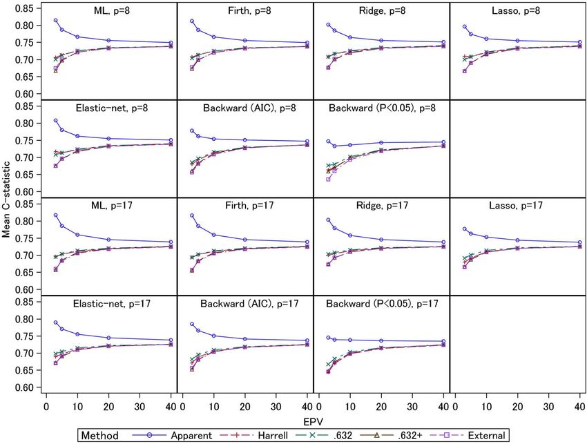
Iba et al. BMC Medical Research Methodology   (2021) 21:9                                                             Page 2 of 14

 (Continued from previous page)
 Conclusions: In general, the three bootstrap estimators were comparable, but the .632+ estimator performed
 relatively well under small sample settings, except when the regularized estimation methods are adopted.
 Keywords: Multivariable clinical prediction model, Optimism, C-statistic, Regularized estimation, Bootstrap

Background                                                       method [8, 9] for estimating regression coefficients, and
Multivariable prediction models have been important              concluded that the .632+ estimator performed especially
statistical tools to provide synthetic diagnosis and prog-       well. Several other modern effective estimation methods
nostic algorithms based on the characteristics of mul-           have been widely adopted in clinical studies. Representa-
tiple patients [1]. A multivariable prediction model is          tive approaches include regularized estimation methods
usually constructed using an adequate regression model           such as ridge [10], lasso (least absolute shrinkage and
(e.g., a logistic regression model for a binary outcome)         selection operator) [11], and elastic-net [12]. Also, conven-
based on a series of representative patients, but it is well     tional stepwise variable selections are still widely adopted
known that their “apparent” predictive performances              in current practice [13]. Note that the previous studies of
such as discrimination and calibration calculated in the         these various estimation methods did not assess the
derivation dataset are better than the actual performance        comparative effectiveness of the bootstrapping estimators.
for an external population [2]. This bias is known as            Also, their simulation settings were not very comprehen-
“optimism” in prediction models. Practical guidelines            sive because their simulations were conducted to assess
(e.g., the Transparent Reporting of a multivariable pre-         various methods and outcome measures, and comparisons
diction model for Individual Prognosis Or Diagnosis              of the bootstrap estimators comprised only part of their
(TRIPOD) statements [2, 3]) recommend optimism ad-               analyses.
justment using principled internal validation methods,              In this work, we conducted extensive simulation
e.g., split-sample, cross-validation (CV), and bootstrap-        studies to provide statistical evidence concerning the
based corrections. Among these validation methods,               comparative effectiveness of the bootstrapping estimators,
split-sample analysis is known to provide a relatively           as well as to provide recommendations for their practical
imprecise estimate, and CV is not suitable for some              use. In particular, we evaluated these methods using
performance measures [4]. Thus, bootstrap-based methods          multivariable prediction models that were developed with
are a good alternative because they provide stable estimates     various model building strategies: conventional logistic re-
for performance measures with low biases [2, 4].                 gression (ML), stepwise variable selection, Firth’s penalized
  In terms of bootstrapping approaches, there are three          likelihood, ridge, lasso, and elastic-net. We considered
effective methods to correct for optimism, specifically          extensive simulation settings based on a real-world clinical
Harrell’s bias correction and the .632 and .632+ estima-         study data, the Global Utilization of Streptokinase and
tors [1, 5, 6]. In clinical studies, Harrell’s bias correction   Tissue plasminogen activator for Occluded coronary arter-
has been conventionally applied for internal validation,         ies (GUSTO-I) trial Western dataset [14, 15]. Note that we
while the .632 and .632+ estimators are rarely seen in           particularly focused on the evaluation of the C-statistic [16]
practice. This is because the Harrell’s method can be            in this work, since it is the most popular discriminant
implemented by a relatively simple algorithm (it can be          measure in clinical prediction models, because the simula-
implemented by rms package in R) and the two                     tion data should be too rich for the extensive studies; the
methods were reported to have similar performances               generalizations to other performance measures would be
with the Harrell’s method in previous simulation studies         discussed in the Discussion section.
[4]. These three estimators are derived from different
concepts, and may exhibit different performances under           Methods
realistic situations. Several simulation studies have been       Model-building strategies for multivariable prediction
conducted to assess their comparative effectiveness.             models
Steyerberg et al. [4] compared these estimators for ordin-       At first, we briefly introduce the estimating methods for the
ary logistic regression models with the maximum likeli-          multivariable prediction models. We consider constructing
hood (ML) estimate, and reported that their performances         a multivariable prediction model for a binary outcome yi
were not too different under relatively large sample set-        (yi = 1: event occurring, or 0: not occurring) (i = 1, 2, …, n).
tings. Further, Mondol and Rahman [7] conducted similar          A logistic regression model πi = 1/(1 + exp(−βTxi)) is widely
simulation studies to assess their performances under rare       used as a regression-based prediction model for the
event settings in which event fraction is about 0.1 or           probability of event occurrence πi = Pr(yi = 1| xi) [2, 17]. xi =
lower. They also considered Firth’s penalized likelihood          (1, xi1, xi2, …, xip)T (i = 1, 2, …, n) are p predictor variables
Iba et al. BMC Medical Research Methodology   (2021) 21:9                                                            Page 3 of 14

for an individual i and β = (β0, β1, …, βp)T are the regression    variable selections were performed using the stats and
coefficients containing the intercept. Plugging an appropri-       logistf packages [31]. Firth’s logistic regression was
ate estimate β  ^ of β into the above model, the estimated         also conducted using the logistf package [31]. The
              ^
probability π i (i = 1, 2, …, n) is defined as the risk score of   ridge, lasso, and elastic-net regressions were performed
individual patients, and this score is used as the criterion       using the glmnet package [32]; the turning parame-
score to determine the predicted outcome.                          ters were consistently determined using the 10-fold
   The ordinary ML estimation can be easily implementable          CV of deviance.
by standard statistical software and has been widely
adopted in practice [2, 17]. However, the ML-based model-          C-statistic and the optimism-correction methods based on
ling strategy is known to have several finite sample prob-         bootstrapping
lems (e.g., overfitting and (quasi-)complete separation)           C-statistic
when applied to a small or sparse dataset [9, 18–20]. Both         Secondly, we review the internal validation methods
properties disappear with increasing events per variables          used in the numerical studies. We focused specifically
(EPVs), defined as the ratio of the number of events to the        on the C-statistic in our numerical evaluations, as it is
number of predictor variables (p) of the prediction model.         most frequently used in clinical studies as an summary
EPV has been formally adopted as a sample size criterion           measure of the discrimination of prediction models [2].
for model development, and in particular, EPV ≥ 10 is a            The C-statistic is defined as the empirical probability
widely adopted criterion [21]; recent studies showed that          that a randomly selected patient who has experienced an
the validity of this criterion depended on case-by-case con-       event has a larger risk score than a patient who has not
ditions [4, 13, 22]. As noted below, the following shrinkage       experienced the event [16]. The C-statistic also corre-
estimation methods can moderate these problems.                    sponds to a nonparametric estimator of the area under
   For variable selection, backward stepwise selection has         the curve (AUC) of the empirical receiver operating
been generally recommended for the development of                  characteristic (ROC) curve for the risk score. The C-statistic
prediction models [23]. For the stopping rule, the signifi-        ranges from 0.5 to 1.0, with larger values corresponding to
cance level criterion (a conventional threshold is P < .050),      superior discriminant performance.
Akaike Information Criterion (AIC) [24], and Bayesian In-
formation Criterion (BIC) [25] can be adopted. Regarding           Harrell’s bias correction method
AIC and BIC, there is no certain evidence which criterion          The most widely applied method for bootstrapping opti-
is absolutely better in practices. However, several previous       mism correction is Harrell’s bias correction [1], which is
studies have reported AIC was more favorable [23, 26, 27],         obtained by the conventional bootstrap bias correction
and thus we adopted only AIC in our simulation studies.            method [4]. The algorithm is summarized as follows:
   Several shrinkage estimation methods such as Firth’s
logistic regression [8], ridge [10], lasso [11], and elastic-         Let θapp be the apparent predictive performance
net [12] have been proposed. These shrinkage methods                    estimate for the original population.
estimate the regression coefficients based on penalized               Generate B bootstrap samples by resampling with
log likelihood function. These methods can deal with                    replacement from the original population.
(quasi-)complete separation problem [9, 17]. Also, since the          Construct a prediction model for each bootstrap
estimates of the regression coefficients are shrunk towards            sample, and calculate the predictive performance
zero, these methods can alleviate overfitting [17, 28, 29].            estimate for it. We denote the B bootstrap estimates
Lasso and elastic-net can shrink some regression coeffi-               as θ1, boot, θ2, boot, ⋯, θB, boot.
cients to be exactly 0; therefore, lasso and elastic-net can          Using the B prediction models constructed from the
perform shrinkage estimation and variable selection simul-             bootstrap samples, calculate the predictive
taneously [11, 12]. The penalized log likelihood function of           performance estimates for the original population:
ridge, lasso, and elastic-net include a turning parameter to           θ1, orig, θ2, orig, ⋯, θB, orig.
control the degree of shrinkage [10–12]. Elastic-net also             The bootstrap estimate of optimism is obtained as
has a turning parameter to determine the weight of lasso
type and ridge type penalties [12]. Several methods, such as
                                                                            1X B
CV, were proposed for selection of the tuning parameters              Λ¼          θb;boot − θb;orig
                                                                            B b¼1
of ridge, lasso, and elastic-net [17, 28, 29].
   In numerical analyses in the following sections, all of
the above methods were performed using R version 3.5.1
language programming (The R Foundation for Statistical               Subtracting the estimate of optimism from the apparent
Computing, Vienna, Austria) [30]. The ordinary logistic            performance, the bias corrected predictive performance
regression was fitted by the glm function. The stepwise            estimate is obtained as θapp − Λ.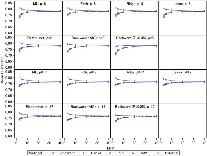
Iba et al. BMC Medical Research Methodology   (2021) 21:9                                                        Page 4 of 14

   The bias correction estimator is calculable by a rela-     when the degree of overfitting is large. Then, the .632+
tively simple algorithm, and some numerical evidence          estimator [6] is defined as
has shown that it performs well under relatively large
sample settings (e.g., EPV ≥ 10) [4]. Therefore, this algo-       θ:632þ ¼ ð1 − wÞ  θapp þ w  θout
rithm is currently adopted in most clinical prediction                      :632
model studies that conduct bootstrap-based internal               w¼
                                                                       1 − :368  R
validations. However, a certain proportion of patients in
the original population (on average, 63.2%) should be           Note that the weight w ranges from .632 (R = 0) to 1
overlapped in the bootstrap sample [6]. The overlap may       (R = 1). Hence, the .632+ estimator approaches the .632
cause overestimation of the predictive performance [27],      estimator when there is no overfitting and approaches
and several alternative estimators have therefore been        the external sample estimate θout when there is marked
proposed, as follows.                                         overfitting.
                                                                In the following numerical studies, the numbers of
Efron’s .632 method                                           bootstrap resamples were consistently set to B = 2000.
Efron’s .632 method [5] was proposed as a bias-               Also, for the model-building methods involving variable
corrected estimator that considers overlapped samples.        selections (e.g., stepwise regression) and shrinkage
Among the B bootstrap samples, we consider the “exter-        methods which require tuning parameter selections
nal” samples that are not included in the bootstrap sam-      (ridge, lasso, and elastic-net), all estimation processes
ples to be ‘test’ datasets for the developed B prediction     were included in the bootstrapping analyses in order to
models. Then, we calculate the predictive performance         appropriately reflect their uncertainty.
estimates for the external samples by the developed B
prediction models θ1, out, θ2, out, ⋯, θB, out, and we de-    Real-data example: applications to the GUSTO-I trial
                                     P
note the average measure as θout ¼ Bb¼1 θb;out =B. There-     Western dataset
after, the .632 estimator is defined as a weighted average    Since we consider the GUSTO-I trial Western dataset as
of the predictive performance estimate in the original        a model example for the simulation settings, we first
sample θapp and the external sample estimate θout:            illustrate the prediction model analyses for this clinical
                                                              trial. The GUSTO-I dataset has been adopted by many
    θ:632 ¼ 0:368  θapp þ 0:632  θout                       performance evaluation studies of multivariable prediction
                                                              models [4, 13, 29], and we specifically used the West re-
  The weight .632 derives from the approximate propor-        gion dataset [23]. GUSTO-I was a comparative clinical
tion of subjects included in a bootstrap sample. Since        trial to assess four treatment strategies for acute myocar-
the subjects that are included and not included in a          dial infarction [14]. Here we adopted death within 30 days
bootstrap sample are independent, the .632 estimator          as the outcome variable (binary). The summary of the
can be interpreted as an extension of CV [4, 7]. How-         outcome and the 17 covariates are presented in Table 1.
ever, the .632 estimator is associated with overestimation    Of the 17 covariates, two variables (height and weight) are
bias under highly overfit situations, when the apparent       continuous, one variable (smoking) is ordinal, and the
estimator θapp has a large bias [6].                          remaining 14 variables are binary; age was dichotomized
                                                              at 65 years old. For smoking, which is a three-category
Efron’s .632+ method                                          variable (current smokers, ex-smokers, and never
Efron and Tibshirani [6] proposed the .632+ estimator         smokers), we generated two dummy variables (ex-smokers
to address the problem of the .632 estimator by taking        vs. never smokers, and current smokers vs. never smokers)
into account the amount of overfitting. They define the       and used them in the analyses.
relative overfitting rate R as                                   We considered two modelling strategies: (1) 8-predictor
                                                              models (age > 65 years, female gender, diabetes, hypotension,
         θout − θapp                                          tachycardia, high risk, shock, and no relief of chest pain),
    R¼
          γ − θapp                                            which was adopted in several previous studies [4, 33]; and (2)
                                                              17-predictor models which included all variables presented
  γ corresponds to ‘no information performance’, which        in Table 1. The EPVs for these models were 16.9 and 7.5,
is the predictive performance measure for the original        respectively. For the two modelling strategies, we constructed
population when the outcomes are randomly permuted.           multivariable logistic prediction models using the estimating
Although the γ can be set to an empirical value, we used      methods in the Methods section (ML, Firth, ridge, lasso,
γ = 0.50 that is the theoretical value for the case of the    elastic-net) and backward stepwise methods with AIC
C-statistic [4]. The overfitting rate R approaches 0 when     and statistical significance (P < 0.05). We also calculated the
there is no overfitting (θout = θapp), and approaches 1       C-statistics and the bootstrap-based optimism-corrected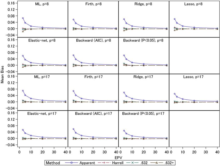
Iba et al. BMC Medical Research Methodology             (2021) 21:9                                                            Page 5 of 14

Table 1 Characteristics of the GUSTO-I Western dataset                        These results indicate that the 17-predictor model had
N                                                              2188           greater optimism, possibly due to the inclusion of noise
Outcome                                                                       variables.
    30-day mortality                                           6.2%
                                                                              Simulations
Covariates
                                                                              Data generation and simulation settings
    Age > 65 years                                             38.4%          As described in the previous section, we conducted ex-
    Female gender                                              24.9%          tensive simulation studies to assess the bootstrap-based
    Diabetes                                                   14.3%          internal validation methods based on a real-world data-
    Hypotension (systolic blood pressure < 100 mmHg)           9.6%           set, the GUSTO-I Western dataset. We considered a
    Tachycardia (pulse > 80 bpm)                               33.4%
                                                                              wide range of conditions with various factors that can
                                                                              affect predictive performance: the EPV (3, 5, 10, 20, and
    High risk (anterior infarct location/previous MI)          48.7%
                                                                              40), the expected event fraction (0.5, 0.25, 0.125, and
    Shock (Killip class III/IV)                                1.5%           0.0625), the number of candidate predictors (eight
    Time to relief of chest pain > 1 h                         60.9%          variables, as specified in the previous studies, and all 17
    Previous MI                                                17.1%          variables), and the regression coefficients of the pre-
    Height (cm)                                                172.1 ± 10.1   dictor variables (two scenarios, as explained below). All
    Weight (kg)                                                82.9 ± 17.7
                                                                              combinations of these settings were covered, and a total
                                                                              of 80 scenarios were investigated. The settings of the
    Hypertension history                                       40.4%
                                                                              EPV and the event fraction were based on those used in
    Ex-smoker                                                  30.8%          previous studies [4, 17]. For the regression coefficients
    Current smoker                                             27.9%          of the predictor variables (except for the intercept β0),
    Hypercholesterolemia                                       40.5%          we considered two scenarios: one fixed to the ML
    Previous angina pectoris                                   34.1%          estimate for the GUSTO-I Western dataset (scenario 1)
    Family history of MI                                       47.6%
                                                                              and the other fixed to the elastic-net estimate for the
                                                                              GUSTO-I Western dataset (scenario 2). In scenario 1, all
    ST elevation in > 4 leads                                  35.6%
                                                                              the predictors have some effect on the risk of events,
                                                                              while in scenario 2 some of the predictor effects are null
estimates for these prediction models. The results are                        and the others are relatively small compared with
presented in Table 2.                                                         scenario 1. The intercept β0 was set to properly adjust
  For the 8-predictor models, the lasso and elastic-net                       the event fractions. The sample size of the derivation cohort
models selected all eight variables. Also, the two back-                      n was determined by (the number of candidate predictor
ward stepwise methods selected the same six variables                         variables × EPV) / (expected event fraction).
for the 8-predictor models; only ‘diabetes’ and ‘no relief                      The predictor variables were generated as random
of chest pain’ were excluded. Further, for the 17-                            numbers based on the parameters estimated from the
predictor models, the lasso and elastic-net models                            GUSTO-I Western dataset. Three continuous variables
selected the same 12 variables, while ‘diabetes’, ‘height’,                   (height, weight, and age) were generated from a multi-
‘hypertension history’, ‘ex-smoker’, ‘hypercholesterolemia’,                  variate normal distribution with the same mean vector
and ‘family history of MI’ were excluded. For the back-                       and covariance matrix as in the GUSTO-I Western data;
ward stepwise selections, the AIC method selected nine                        the age variable was dichotomized at age 65 years,
variables and the significance-based method selected                          similar to the analyses in the real-data example. For
seven variables; see Table 2 for the selected variables.                      smoking, an ordinal variable, random numbers were
  In general, the apparent C-statistics of the 17-predictor                   generated from multinomial distribution using the same
models were larger than those of the 8-predictor models.                      proportions as in the GUSTO-I Western data; this vari-
Although the apparent C-statistics of all the prediction                      able was converted to two dummy variables before being
models were comparable for the 8-predictor models                             incorporated into the prediction models. In addition, the
(about 0.82), the apparent C-statistics of the 17-predictor                   remaining binary variables were generated from a multi-
models were ranged from 0.82 to 0.83. The optimism-                           variate binomial distribution [34] using the same mar-
corrected C-statistics (about 0.81) were smaller than the                     ginal probabilities and correlation coefficients estimated
apparent C-statistics for all models, and certain biases                      from the GUSTO-I Western dataset. We used the
were discernible. However, among the three bootstrapping                      mipfp package [35] for generating the correlated bino-
methods, there were no differences for any of the predic-                     mial variables. The event occurrence probability πi (i = 1,
tion models. Note that the optimism-corrected C-statistics                    2, …, n) was determined based on the generated predictor
between the 8- and 17-predictor models were comparable.                       variables xi and the logistic regression model πi = 1/(1 +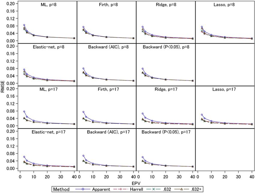
Table 2 Regression coefficients estimates and predictive performance measures for the GUSTO-I trial Westen dataset
                               8-Predictor Model                                                           17-Predictor Model
                               ML       Firth      Ridge    Lasso    Elastic-net   Backward   Backward     ML       Firth       Ridge    Lasso    Elastic-net   Backward   Backward
                                                                                   (AIC)      (P < 0.05)                                                        (AIC)      (P < 0.05)
Coefficients:
   Intercept                   −5.092   −5.034     −4.787   −4.933   − 4.886       − 4.927    − 4.927      −5.090   −4.983      −3.434   −3.494   −3.486        −3.494     −2.853
   Age > 65 years              1.637    1.616      1.424    1.578    1.535         1.631      1.631        1.429    1.399       1.161    1.336    1.324         1.495      1.532
   Female gender               0.622    0.620      0.592    0.586    0.586         0.624      0.624        0.490    0.487       0.380    0.288    0.289         0.368      .
                                                                                                                                                                                        Iba et al. BMC Medical Research Methodology

   Diabetes                    0.069    0.083      0.078    0.024    0.035         .          .            0.153    0.164       0.131    .        .             .          .
   Hypotension                 1.218    1.215      1.102    1.164    1.145         1.252      1.252        1.192    1.178       1.037    1.036    1.030         1.230      1.227
   Tachycardia                 0.650    0.645      0.574    0.608    0.597         0.661      0.661        0.653    0.643       0.533    0.530    0.526         0.669      0.717
   High risk                   0.847    0.835      0.748    0.796    0.781         0.855      0.855        0.403    0.397       0.390    0.372    0.372         0.414      2.748
                                                                                                                                                                                        (2021) 21:9

   Shock                       2.395    2.362      2.339    2.362    2.354         2.424      2.424        2.685    2.608       2.508    2.460    2.455         2.662      0.779
   No relief of chest pain     0.263    0.255      0.237    0.219    0.221         .          .            0.233    0.223       0.200    0.107    0.107         .          .
   Previous MI                                                                                             0.505    0.495       0.437    0.378    0.376         0.586      .
   Height                                                                                                  0.008    0.008       −0.001   .        .             .          .
   Weight                                                                                                  −0.019   −0.018      −0.015   −0.014   −0.014        −0.018     −0.023
   Hypertension history                                                                                    −0.165   −0.159      −0.123   .        .             .          .
   Ex-smoker                                                                                               0.174    0.169       0.147    .        .             .          .
   Current smoker                                                                                          0.247    0.241       0.231    0.057    0.059         .          .
   Hypercholesterolemia                                                                                    −0.064   −0.060      −0.064   .        .             .          .
   Previous angina pectoris                                                                                0.246    0.243       0.235    0.151    0.151         .          .
   Family history of MI                                                                                    −0.015   −0.014      −0.036   .        .             .          .
   ST elevation in > 4 leads                                                                               0.583    0.571       0.479    0.434    0.430         0.601      0.752
C-statistics:
   Apparent                    0.819    0.819      0.819    0.819    0.819         0.820      0.820        0.832    0.832       0.831    0.831    0.831         0.829      0.824
   Harrell                     0.810    0.810      0.812    0.810    0.810         0.811      0.810        0.811    0.811       0.812    0.812    0.812         0.810      0.806
   .632                        0.811    0.811      0.812    0.811    0.810         0.811      0.809        0.811    0.811       0.813    0.813    0.813         0.809      0.808
   .632+                       0.810    0.811      0.812    0.811    0.810         0.811      0.809        0.810    0.810       0.812    0.812    0.812         0.809      0.808
                                                                                                                                                                                        Page 6 of 14
Iba et al. BMC Medical Research Methodology (2021) 21:9 Page 7 of 14
exp(−βTxi)). The outcome variable yi was generated from for EPV = 3 and 5, and around 0.72 for larger EPV.
a Bernoulli distribution with a success probability πi. These results were similar between the 8- and 17-predictor
The actual prediction performances of the developed models. For the 17-predictor models under EPV = 3, the
models were assessed by 500,000 independently gener- ridge, lasso, and elastic-net showed large external C-statis-
ated external test samples; the empirical C-statistics for tics (0.67) compared with the other models. The external
the test datasets, which we refer to as the ‘external’ C- C-statistics for the ML estimation, Firth regression, and
statistics, were used as the estimands. The number of stepwise selection (AIC) were comparable (0.66). The step-
simulations was consistently set to 2000 for all the sce- wise selection (p< 0.05) had the smallest external C-statistic
narios. Based on the generated derivation cohort dataset, (0.65). For the 8-predictor models under EPV = 3, the
the multivariable prediction models were constructed external C-statistics for the ridge, elastic-net, and Firth
using the seven modelling strategies (ML, Firth, ridge, regression were comparable (0.68). However, the external
lasso, elastic-net, and backward stepwise selections with C-statistic for the lasso was similar to that for the ML esti-
AIC and P < 0.05). The C-statistics for the derivation co- mation (0.67). Both stepwise selections had small external
hort were estimated by the apparent, Harrell, .632, and C-statistics (0.64–0.66) compared with the other models. In
.632+ bootstrapping methods in the derivation cohort. general, the shrinkage methods showed better actual pre-
For the evaluation measures, biases and RMSEs (root dictive performances than the other methods. In particular,
mean squared errors) for the estimated C-statistics from for the 17-predictor models with the noise variables, the
the external C-statistic for the 500,000 test datasets were ridge, lasso, and elastic-net had better predictive perfor-
used. mances compared with the Firth method. However, the
In order to assess sensitivity to involve skewed lasso did not perform well for the 8-predictor models. This
continuous variables as predictors, the three continuous might be caused by total sample size; the scenarios for the
variables were also generated from a multivariate skew 8-predictor models had smaller total sample size. Although
normal distribution [36] with the parameters estimated the Firth regression showed better predictive performance
from the GUSTO-I Western dataset. The sensitivity ana- compared with the ML estimation for the 8-predictor
lyses for the skewed variables settings were conducted models, the predictive performances of the Firth and ML
only for the ML estimation. methods were comparable for the 17-predictor models.
Further, the predictive performances of stepwise selections
were generally worse than the other methods, as shown by
Simulation results previous studies [17]. Similar trends were observed under
In the main Tables and Figures, we present the results event fraction = 0.0625, but the external C-statistics
of scenario 2 with event fractions of 0.5 and 0.0625; as (around 0.75, under EPV = 3–5) were larger than those
mentioned below, the overall trends were not very differ- under event fraction = 0.5. These results were caused by
ent, and these scenarios are representative of the all the total sample sizes: the event fraction of the latter
simulation results. Other simulation results are provided scenario was smaller and the total sample sizes were larger
in e-Appendix A in Additional file 1 because the con- if EPV were the same. Comparing the modelling strategies,
tents were too large to present in this manuscript. In the the similar trends as those under event fraction = 0.5 were
small-sample settings (low EPVs and large event frac- observed.
tions), the simulation results for modelling strategies in- In Figs. 3 and 4, we present the empirical biases of
volving variable selections (lasso, elastic-net, and the estimators of C-statistics derived from the exter-
stepwise selections) occasionally dropped all of the pre- nal C-statistics. Under EPV = 3 and 5, the apparent
dictors; in such cases, only an intercept remained, yield- C-statistics had large overestimation biases (0.07–0.16
ing a nonsensical prediction model. We excluded these for event fraction = 0.5 and 0.03–0.07 for event frac-
cases from the performance evaluations because such tion = 0.0625) compared with the three bootstrapping
models are not usually adopted in practice. As reference methods. In particular, under smaller EPV settings,
information, the frequencies with which the intercept the overestimation biases were larger. For the same
models occurred are presented in e-Table 1 in e- EPV settings, the overestimation biases were smaller
Appendix B in Additional file 1. The results of the sensi- when the event fraction was smaller (i.e., the total
tivity analyses for skewed variables settings are presented sample sizes were larger). For 17-predictor models
in e-Appendix C in Additional file 1. under event fraction = 0.5 and EPV = 3, the overesti-
The average values of the apparent, external, and mation biases of the apparent C-statistics of the ML
optimism-corrected C-statistics for 2000 simulations are and Firth methods (0.16) were larger than those of
shown in Fig. 1 (for event fraction = 0.5) and Fig. 2 (for the other methods. The ridge and AIC method had
event fraction = 0.0625). Under event fraction = 0.5, the large overestimation biases (0.13) compared with the
external C-statistics for the test datasets were 0.65–0.70 elastic-net and lasso (0.11–0.12). The P < 0.05Iba et al. BMC Medical Research Methodology (2021) 21:9 Page 8 of 14 Fig. 1 Simulation results: apparent, external, and optimism-corrected C-statistics (scenario 2 and event fraction = 0.5) criterion had the smallest overestimation bias (0.10). overestimation biases (0.01 or lower). For the 17- For 8-predictor models, the ML estimation showed predictor models, the underestimation biases of the large overestimation bias (0.14) compared with the .632+ estimator were less than 0.01, but in general other methods. The overestimation biases of the this estimator displayed underestimation biases. The shrinkage methods were comparable (0.13). The step- Harrell and .632 estimators had overestimation biases wise selections had small overestimation biases (0.11– (less than 0.01). Under event fraction = 0.5, the over- 0.12) compared with other methods, but the external estimation biases of the Harrell and .632 estimators C-statistics were also smaller, as noted above. Gener- were remarkably large under EPV = 3 and 5; under ally, similar trends were observed for event fraction = the 8-predictor models, the overestimation biases 0.0625. Comparing the three bootstrapping methods were 0.03–0.04. Although the .632+ estimator had under EPV ≥ 20, the biases of all the methods were underestimation biases for the ML and Firth methods comparable for all settings. The results for the con- (0.01 under EPV = 3), mostly unbiased estimates were ventional ML estimation were consistent with those obtained for the ridge, lasso, and elastic-net estima- of Steyerberg et al. (2001) [4], and we confirmed that tors. For the stepwise selections, the AIC method similar results were obtained for the shrinkage esti- provided mostly unbiased estimator, but the P < 0.05 mation methods. Further, under small EPV settings, criterion resulted in overestimation bias (0.02). For unbiased estimates were similarly obtained by the the 17-predictor models, similar trends were observed. three bootstrapping methods for the 8-predictor The Harrell and .632 estimators had overestimation models with event fraction = 0.0625, since the total biases (0.02–0.04 under EPV = 3), and the two esti- sample size was relatively large, and similar trends mators were comparable for the ML, Firth, and ridge were observed for all estimation methods under EPV estimators. However, for the lasso, elastic-net, and ≥ 5. Under EPV = 3, the .632+ estimator had under- stepwise (AIC) methods, whereas the overestimation estimation biases, while for the ML estimation, the biases of the Harrell estimator were 0.02, those of the underestimation bias was 0.02. For ridge, lasso, and .632 estimator were 0.03. For the stepwise selection elastic-net, the underestimation biases were 0.01. For method (P < 0.05), the .632 estimator showed over- the Firth regression and stepwise methods, the under- estimation bias (0.02), but the Harrell estimator was estimation biases were less than 0.01. The Harrell and mostly unbiased. Further, the .632+ estimator had .632 estimators were comparable, and they had underestimation biases (less than 0.01) for the ML,
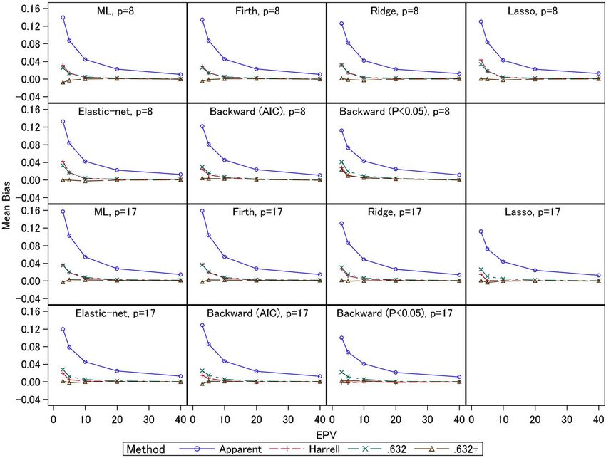
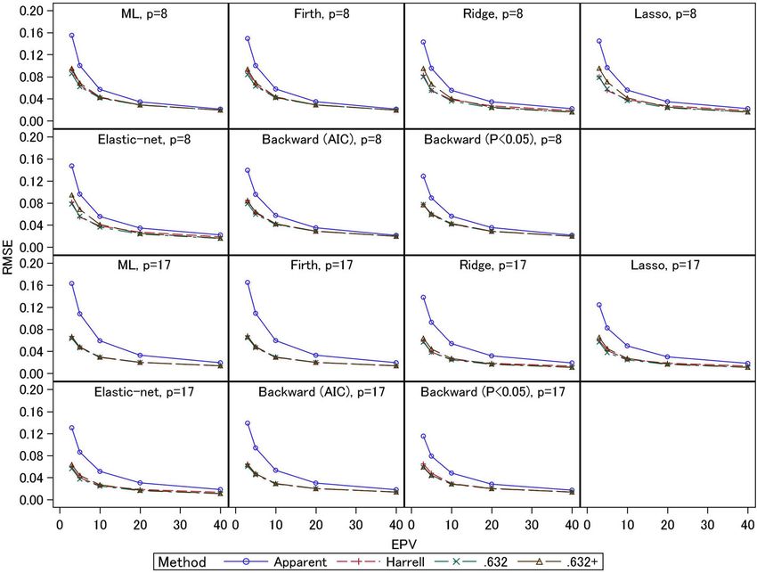
Iba et al. BMC Medical Research Methodology          (2021) 21:9                                                               Page 9 of 14

 Fig. 2 Simulation results: apparent, external, and optimism-corrected C-statistics (scenario 2 and event fraction = 0.0625)

Firth, and stepwise (AIC) methods; this estimator was                         scenarios in which the biases of the .632+ estimator
mostly unbiased for the ridge, lasso, elastic-net, and                        were smaller than those of the other two estimators,
stepwise (P < 0.05) methods.                                                  and in these cases the RMSEs were comparable with
   The empirical RMSEs are presented in Figs. 5 and 6.                        those of the Harrell and .632 estimators. These results
Under EPV = 3 and 5, the apparent C-statistics had large                      indicate the .632+ estimator had large standard errors
RMSEs (0.08–0.16 for event fraction = 0.5 and 0.04–0.08                       compared with the other two estimators when EPV
for event fraction = 0.0625) compared with the three                          were small.
bootstrapping methods; these large RMSEs of the ap-                             The results described above are mostly consistent with
parent C-statistics were caused by their large overesti-                      those derived under the other settings presented in the
mation biases under small EPV, as noted above. The                            e-Appendix A in the Additional file 1.
RMSEs of the three bootstrapping methods were gen-
erally comparable. An exception is that under event                           Discussion
fraction = 0.5 and EPV = 3 and 5, the RMSEs of the                            Bootstrapping methods for internal validations of dis-
.632+ estimators of the 8-predictor models with ridge,                        criminant and calibration measures in developing
lasso, and elastic-net (0.07–0.10) were larger than                           multivariable prediction models have been increas-
those of the other two estimators (0.05–0.08). As                             ingly used in recent clinical studies. The Harrell, .632,
mentioned above, under these conditions the absolute                          and .632+ estimators are asymptotically equivalent
biases of the .632+ estimators were smaller, reflecting                       (e.g., they have same biases and RMSEs under large
these estimators’ standard errors. For the 17-predictor                       sample setting), but in practice they might have dif-
models, the RMSEs were comparable. Under event                                ferent properties in finite sample situations (e.g., the
fraction = 0.0625, the .632+ estimators for ridge,                            directions and sizes of biases of these estimators are
lasso, and elastic-net had large RMSEs (0.06–0.07)                            inconsistent in small sample setting). This fact may
compared with the other two estimators (0.05) for the                         influence the main conclusions of relevant studies,
8-predictor models under EPV = 3. These results re-                           and conclusive evidence of these estimators’ compara-
flect the fact that under these conditions, the absolute                      tive effectiveness is needed to ensure appropriate re-
biases of the .632+ estimators were larger than those                         search practices. In this work, we conducted extensive
of the other two estimators. In addition, under the                           simulation studies to assess these methods under a
other settings with small EPV, there were many                                wide range of situations. In particular, we assessed
Iba et al. BMC Medical Research Methodology         (2021) 21:9                                                              Page 10 of 14

 Fig. 3 Simulation results: bias in the apparent and optimism-corrected C-statistics (scenario 2 and event fraction = 0.5)

their properties in the context of the prediction                              Among the bootstrapping optimism-correction
models developed by modern shrinkage methods                                 methods, we showed that the Harrell and .632 methods
(ridge, lasso, and elastic-net), which are becoming                          had upward biases at EPV = 3 and 5. The biases in these
increasingly more popular. We also evaluated stepwise                        methods increased when the event fraction became lar-
selections, which are additional standard methods of                         ger. As mentioned in the Methods section, the overlap
variable selection, taking into consideration the uncer-                     between the original and bootstrap samples under small
tainties of variable selection processes.                                    sample settings could cause these biases. Therefore,
  Conventionally, the rule-of-thumb criterion for sample                     these methods should be used with caution in cases of
size determination in prediction model studies is EPV ≥                      small sample settings. When the event fraction was 0.5,
10 [21]. In our simulations, the internal validation                         the .632 estimator often had a greater upward bias than
methods generally worked well under these settings.                          the Harrell method for the shrinkage estimating
However, several counterexamples were reported in                            methods and stepwise selections. Similarly, the .632+ es-
previous studies [4, 13, 22], so this should not be an                       timator showed upward biases at EPV = 3 for the step-
absolute criterion. There were certain conditions in                         wise selection (P < 0.05) for the 8-predictor model. Since
which the standard logistic regression performed well                        the .632+ estimator is constructed by a weighted average
under EPV < 10; relative bias (percentage difference from                    of the apparent performance and the out-of-sample per-
true value) of the standard logistic regression was 15%                      formance measures, it cannot have a negative bias when
or lower [22]. Also, EPV ≥ 10 criterion might not be                         the resultant prediction model has extremely low pre-
sufficient for the stepwise selections [13]. The external                    dictive performance, i.e., when the apparent C-statistics
C-statistics of the stepwise selections were smaller than                    are around 0.5. However, if such a prediction model is
those of ML estimation under certain situations, as                          obtained in practice, we should not adopt it as the final
previously discussed [13], and variable selection methods                    model. Note that these results did not commonly occur
might not be recommended in practice. Moreover,                              in the simulation studies. For example, the cases that the
the shrinkage regression methods (ridge, lasso, and                          apparent C-statistics were less than 0.6 did not been ob-
elastic-net) provided larger C-statistics than ML esti-                      served for the settings EPV ≥ 10. For the ridge, lasso,
mation and Firth’s method under certain settings, and                        elastic-net, and stepwise methods, the frequencies these
were generally comparable. Further investigations are                        cases occurred were ranged 0.1–2.1% (median: 0.2%) for
needed to assess the practical value of these methods                        EPV = 5 settings, and 0.1–3.6% (median: 0.4%) for EPV
in clinical studies.                                                         = 3 settings.
Iba et al. BMC Medical Research Methodology         (2021) 21:9                                                                 Page 11 of 14

 Fig. 4 Simulation results: bias in the apparent and optimism-corrected C-statistics (scenario 2 and event fraction = 0.0625)

  Also, since the .632+ estimator was developed to over-                     the RMSE in the Harrell method became larger.
come the problems of the .632 estimator under highly                         These results indicate that the performances of the
overfitted situations, the .632+ estimator is expected to                    optimism-corrected estimators depend on the
have smaller overestimation bias compared with the                           methods of penalty parameter selections. Since the
other two methods. However, the .632+ estimator                              external C-statistics of lasso using the 10-fold CV and
showed a slight downward bias when the event fraction                        the leave-one-out CV were comparable, the leave-
was 0.0625; the relative overfitting rate was overesti-                      one-out CV showed no clear advantage in terms of
mated in that case, since a small number of events was                       penalty parameter selections.
discriminated well by less overfitted models. This ten-                        In this work, we conducted simulation studies based
dency was clearly shown for the ML method, which has                         on the GUSTO-I study Western dataset. We consid-
the strongest overfitting risk.                                              ered a wide range of settings by varying several fac-
  Although the bias of the .632+ estimator was relatively                    tors to investigate detailed operating characteristics of
small, its RMSE was comparable or sometimes larger                           the bootstrapping methods. A limitation of the study
than those of the other two methods. Since the .632+                         is that settings for the predictor variables were based
estimator adjusts the weights of apparent and out-of-                        only on the case of the GUSTO-I study Western
sample performances using the relative overfitting                           dataset which evaluated mortality in patients with
rate, the .632+ estimator has variations due to the                          acute myocardial infarction, and these settings were
variability of the estimated models under small sam-                         adopted throughout all scenarios. Thus, the results
ple settings. Also, the RMSE of the .632+ estimator                          from our simulation studies cannot be generalized to
was particularly large in the shrinkage estimation                           other cases straightforwardly. Also, we considered
methods; the penalty parameters were usually selected                        only the 8- and 17-predictor models that were
by 5- or 10-fold CV and we adopted the latter in our                         adopted in many previous studies [4, 13, 29]. Al-
simulations. Since the 10-fold CV is unstable with                           though other scenarios could be considered, the
small samples [37], the overfitting rate often has large                     computational burden of the simulations studies was
variations. We attempted to use the leave-one-out CV                         quite enormous; it requires total 4,000,000 iterations
instead of the 10-fold CV, and this decreased the                            (2000 replication × 2000 bootstrap resampling) in
RMSE of the .632+ estimator (see e-Table 2 in e-                             each scenario. Considerations of other scenarios or
Appendix B in Additional file 1). On the other hand,                         datasets would be further issues in future studies. In
Iba et al. BMC Medical Research Methodology         (2021) 21:9                                                                 Page 12 of 14

 Fig. 5 Simulation results: RMSE in the apparent and optimism-corrected C-statistics (scenario 2 and event fraction = 0.5)

 Fig. 6 Simulation results: RMSE in the apparent and optimism-corrected C-statistics (scenario 2 and event fraction = 0.0625)
Iba et al. BMC Medical Research Methodology             (2021) 21:9                                                                               Page 13 of 14

addition, we assessed only the C-statistic in this                             Cancer Control (Grant number: 17ck0106266) from the Japan Agency for
study. Other measures such as the Brier score and                              Medical Research and Development, and the JSPS KAKENHI (Grant numbers:
                                                                               JP17H01557 and JP17K19808).
calibration slope can also be considered for the evalu-                        The funders have no involvement in study design, data collection or analysis,
ation of optimism corrections. However, in previous                            interpretation or writing of the manuscript.
simulation studies, these measures showed similar
trends [4]. Also, the partial area under the ROC curve                         Availability of data and materials
                                                                               The GUSTO-I Western dataset is available at http://www.clinicalprediction
is another useful discriminant measure that can assess                         models.org.
the predictive performance within a certain range of
interest (e.g., small false positive rate or high true                         Ethics approval and consent to participate
positive rate) [38, 39]. Its practical usefulness for mul-                     Not applicable.
tivariable prediction models has not been well investi-
                                                                               Consent for publication
gated, and extended simulation studies would also be                           Not applicable.
a further issue in future studies.
                                                                               Competing interests
                                                                               The authors declare that they have no competing interests.
Conclusions
In conclusion, under certain sample sizes (roughly,                            Author details
EPV ≥ 10), all of the internal validation methods                              1
                                                                                Department of Statistical Science, School of Multidisciplinary Sciences, The
                                                                               Graduate University for Advanced Studies, Tokyo, Japan. 2Office of
based on bootstrapping performed well. However,
                                                                               Biostatistics, Department of Biometrics, Headquarters of Clinical
under small sample settings, all the methods had                               Development, Otsuka Pharmaceutical Co., Ltd., Tokyo, Japan. 3Department of
biases. For the ridge, lasso, and elastic-net methods,                         Information and Computer Technology, Faculty of Engineering, Tokyo
                                                                               University of Science, Tokyo, Japan. 4Department of Biostatistics, Faculty of
although the bias of the .632+ estimator was rela-
                                                                               Medicine, University of Tsukuba, Ibaraki, Japan. 5Department of Data Science,
tively small, its RMSE could become larger than                                The Institute of Statistical Mathematics, 10-3 Midori-cho, Tachikawa, Tokyo
those of the Harrell and .632 estimators. Under small                          190-8562, Japan.
sample settings, the penalty parameter selection strat-
                                                                               Received: 5 March 2020 Accepted: 21 December 2020
egy should be carefully considered; one possibility is
to adopt the leave-one-out CV instead of the 5- or
10-fold CV. For the other estimation methods, the                              References
                                                                               1. Harrell FE, Lee KL, Mark DB. Multivariable prognostic models: issues in
three bootstrap estimators were comparable in general,
                                                                                   developing models, evaluating assumptions and adequacy, and measuring
but the .632+ estimator performed relatively well under                            and reducing errors. Stat Med. 1996;15(4):361–87.
certain settings. In addition, developments of new                             2. Moons KG, Altman DG, Reitsma JB, Ioannidis JP, Macaskill P, Steyerberg EW,
                                                                                   et al. Transparent reporting of a multivariable prediction model for
methods to overcome these issues are future issues to be
                                                                                   individual prognosis or diagnosis (TRIPOD): explanation and elaboration.
investigated.                                                                      Ann Intern Med. 2015;162(1):W1–73.
                                                                               3. Collins GS, Reitsma JB, Altman DG, Moons KG. Transparent reporting of a
                                                                                   multivariable prediction model for individual prognosis or diagnosis
Supplementary Information                                                          (TRIPOD): the TRIPOD statement. Ann Intern Med. 2015;162(1):55–63.
The online version contains supplementary material available at https://doi.
                                                                               4. Steyerberg EW, Harrell FE, Borsboom GJJM, Eijkemans MJC, Vergouwe Y,
org/10.1186/s12874-020-01201-w.
                                                                                   Habbema JDF. Internal validation of predictive models. J Clin Epidemiol.
                                                                                   2001;54(8):774–81.
 Additional file 1.                                                            5. Efron B. Estimating the error rate of a prediction rule: improvement on
                                                                                   cross-validation. J Am Stat Assoc. 1983;78(382):316–31.
                                                                               6. Efron B, Tibshirani R. Improvements on cross-validation: the 632+ bootstrap
Abbreviations                                                                      method. J Am Stat Assoc. 1997;92(438):548–60.
CV: Cross-validation; ML: Maximum likelihood; EPV: Events per variable;        7. Mondol M, Rahman MS. A comparison of internal validation methods for
AIC: Akaike Information Criterion; BIC: Bayesian Information Criterion;            validating predictive models for binary data with rare events. J Stat Res.
AUC: Area under the curve; ROC: Receiver operating characteristic;                 2018;51:131–44.
RMSE: Root mean squared errors                                                 8. Firth D. Bias reduction of maximum likelihood estimates. Biometrika. 1993;
                                                                                   80(1):27–38.
Acknowledgements                                                               9. Heinze G, Schemper M. A solution to the problem of separation in logistic
The authors are grateful to Professor Hideitsu Hino for his helpful comments       regression. Stat Med. 2002;21(16):2409–19.
and advice.                                                                    10. Lee AH, Silvapulle MJ. Ridge estimation in logistic regression. Commun Stat
                                                                                   Simul Comput. 1988;17(4):1231–57.
Authors’ contributions                                                         11. Tibshirani R. Regression shrinkage and selection via the lasso. J R Statist Soc
KI, TS, KM and HN contributed to the review of methodology and planning            B. 1996;58(1):267–88.
of the simulations studies. KI and HN contributed to conduct the real-data     12. Zou H, Hastie T. Regularization and variable selection via the elastic net. J R
analyses and the simulation studies. KI, TS, KM and HN contributed to the          Statist Soc B. 2005;67(2):301–20.
interpretation of data. KI and HN drafted the manuscript. All authors          13. Steyerberg EW, Eijkemans MJC, Harrell FE, Habbema JDF. Prognostic
reviewed, read and approved the final version to be submitted.                     modelling with logistic regression analysis: a comparison of selection and
                                                                                   estimation methods in small data sets. Stat Med. 2000;19(8):1059–79.
Funding                                                                        14. The GUSTO investigators. An international randomized trial comparing four
This work was supported by CREST from the Japan Science and Technology             thrombolytic strategies for acute myocardial infarction. N Engl J Med. 1993;
Agency (Grant number: JPMJCR1412), the Practical Research for Innovative           329(10):673–82.
Iba et al. BMC Medical Research Methodology (2021) 21:9 Page 14 of 14
15. Lee KL, Woodlief LH, Topol EJ, Weaver WD, Betriu A, Col J, et al. Predictors
of 30-day mortality in the era of reperfusion for acute myocardial infarction.
Results from an international trial of 41,021 patients. Circulation. 1995;91(6):
1659–68.
16. Meurer WJ, Tolles J. Logistic regression diagnostics: understanding how well
a model predicts outcomes. JAMA. 2017;317(10):1068–9.
17. van Smeden M, Moons KG, de Groot JA, Collins GS, Altman DG, Eijkemans
MJ, et al. Sample size for binary logistic prediction models: beyond events
per variable criteria. Stat Methods Med Res. 2019;28(8):2455–74.
18. Albert A, Anderson JA. On the existence of maximum likelihood estimates
in logistic regression models. Biometrika. 1984;71(1):1–10.
19. Gart JJ, Zweifel JR. On the bias of various estimators of the logit and its
variance with application to quantal bioassay. Biometrika. 1967;54(1/2):181–7.
20. Jewell NP. Small-sample bias of point estimators of the odds ratio from
matched sets. Biometrics. 1984;40(2):421–35.
21. Peduzzi P, Concato J, Kemper E, Holford TR, Feinstein AR. A simulation study
of the number of events per variable in logistic regression analysis. J Clin
Epidemiol. 1996;49(12):1373–9.
22. Vittinghoff E, McCulloch CE. Relaxing the rule of ten events per variable in
logistic and cox regression. Am J Epidemiol. 2007;165(6):710–8.
23. Steyerberg EW. Clinical prediction models: a practical approach to
development, validation, and updating. New York: Springer; 2019.
24. Akaike H. Information theory and an extension of the maximum likelihood
principle. In: 2nd International Symposium on Information Theory; 1973. p.
267–81.
25. Schwarz G. Estimating the dimension of a model. Ann Stat. 1978;6(2):461–4.
26. Ambler G, Brady AR, Royston P. Simplifying a prognostic model: a
simulation study based on clinical data. Stat Med. 2002;21(24):3803–22.
27. Hastie T, Tibshirani R, Friedman JH. The elements of statistical learning: data
mining, inference, and prediction. New York: Springer; 2009.
28. Rahman MS, Sultana M. Performance of Firth-and logF-type penalized
methods in risk prediction for small or sparse binary data. BMC Med Res
Methodol. 2017;17(1):33.
29. Steyerberg EW, Eijkemans MJC, Habbema JDF. Application of shrinkage
techniques in logistic regression analysis: a case study. Stat Neerl. 2001;55(1):
76–88.
30. R Core Team. R: A language and environment for statistical computing.
Vienna: R Foundation for Statistical Computing; 2018.
31. Heinze G, Ploner M. logistf: Firth’s bias-reduced logistic regression. R
package version 123; 2018.
32. Friedman J, Hastie T, Tibshirani R. Regularization paths for generalized linear
models via coordinate descent. J Stat Softw. 2010;33(1):1–22.
33. Mueller HS, Cohen LS, Braunwald E, Forman S, Feit F, Ross A, et al.
Predictors of early morbidity and mortality after thrombolytic therapy of
acute myocardial infarction. Analyses of patient subgroups in the
thrombolysis in myocardial infarction (TIMI) trial, phase II. Circulation. 1992;
85(4):1254–64.
34. Dai B, Ding S, Wahba G. Multivariate Bernoulli distribution. Bernoulli. 2013;
19(4):1465–83.
35. Barthélemy J, Suesse T. mipfp: An R package for multidimensional array
fitting and simulating multivariate Bernoulli distributions. J Stat Softw. 2018;
86:1–20 (Code Snippet 2).
36. Azzalini A, Capitanio A. The skew-Normal and related families. Cambridge:
Cambridge University Press; 2014.
37. Tantithamthavorn C, McIntosh S, Hassan AE, Matsumoto K. An empirical
comparison of model validation techniques for defect prediction models.
IEEE Trans Softw Eng. 2017;43(1):1–18.
38. Gerds TA, Cai T, Schumacher M. The performance of risk prediction models.
Biom J. 2008;50(4):457–79.
39. Robin X, Turck N, Hainard A, Tiberti N, Lisacek F, Sanchez JC, et al. pROC: an
open-source package for R and S+ to analyze and compare ROC curves.
BMC Bioinform. 2011;12:77.
Publisher’s Note
Springer Nature remains neutral with regard to jurisdictional claims in
published maps and institutional affiliations.You can also read