Getting Started With the R Commander
←
→
Page content transcription
If your browser does not render page correctly, please read the page content below
Getting Started With the R Commander∗
                                       John Fox and Milan Bouchet-Valat

                                Version 2.1-0 (last modified: 22 August 2014)

1      Introduction
The R Commander (Fox, 2005) provides a graphical user interface (“GUI”) to the open-source R statistical
computing environment (R Core Team, 2014). R is a command-driven system, and new users often find
learning R challenging. This is particularly true of those who are new to statistical methods, such as students
in basic-statistics courses. By providing a point-and-click interface to R, the R Commander allows these
users to focus on statistical methods rather than on remembering and generating R commands. Moreover,
by rendering the generated commands visible to users, the R Commander has the potential for easing the
transition to writing R commands, at least for some users. The R Commander, however, accesses only
a small fraction of the capabilities of R and the literally thousands of R packages contributed by users to
the Comprehensive R Archive Network (CRAN). The R Commander is itself extensible through plug-in
packages, and many such plug-ins are now available on CRAN (see Section 6.4 of this document).
    This document directly describes the use of the R Commander under the Windows version of R. There
are small differences in the appearance and use of the R Commander under Mac OS X and on Linux and
Unix systems. Information about installing the R Commander on these platforms is available by following
the link to the installation notes at the R Commander web page  or directly at .
    We use the following typographical conventions in this document: Names of software, such as Windows,
R, the Rcmdr package, and the R Commander, are set in boldface type. The names of GUI elements
such as menus, menu items, windows, and dialog boxes, are set in italic type. Variable names, names of
data sets, and R commands are set in a typewriter font.

2      Starting the R Commander
Once R is running, simply loading the Rcmdr package by typing the command library(Rcmdr) into the
R Console starts the R Commander graphical user interface. To function optimally under Windows, the
R Commander prefers the single-document interface (“SDI”) to R.1 After loading the package, R Console
and R Commander windows should appear more or less as in Figures 1 and 2. These and other screen
images in this document were created under Windows 7; if you use another version of Windows (or, of
course, another computing platform), then the appearance of the screen may differ.2
    ∗ Parts of this manual are adapted and updated from Fox (2005). Please address correspondence to jfox@mcmaster.ca.
    1 The Windows version of R is normally run from a multiple-document interface (“MDI”), which contains the R Console
window, Graphical Device windows created during the session, and other windows related to the R process. In contrast, under
the single-document interface (“SDI”), the R Console and Graphical Device windows are not contained within a master window.
There are several ways to run R in SDI mode — for example, by selecting the SDI when R is installed, by editing the Rconsole
file in R’s etc subdirectory, or by adding --sdi to the Target field in the Shortcut tab of the R desktop icon’s Properties. You
should be able to use the R Commander with the MDI, but it will not appear within the master R window and arranging
the screen will be inconvenient.
    2 Notice that the R Commander requires some packages in addition to several of the “recommended” packages that are

normally distributed with R. The Rcmdr package, the required packages, and many other contributed packages are available
for download from the Comprehensive R Archive Network (CRAN) at
   If these packages are not installed, the R Commander will offer to install them from the Internet or from local files (e.g.,
on a CD/ROM). If you install the Rcmdr package via the Windows “R GUI,” not all of the packages on which the Rcmdr

                                                               1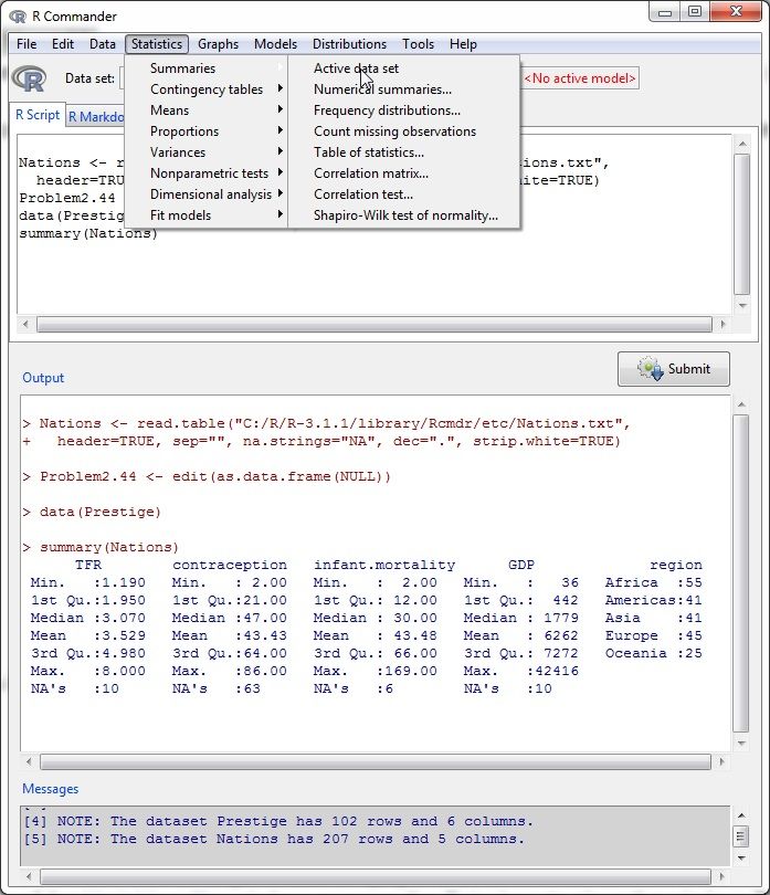
Figure 1: The R Console window after loading the Rcmdr package.

   The R Commander and R Console windows float freely on the desktop. You will normally use the R
Commander’s menus and dialog boxes to read, manipulate, and analyze data, and you can safely minimize
the R Console window.

   • R commands generated by the R Commander GUI appear in the R Script tab in the upper pane
     of the main R Commander window. You can also type R commands directly into the script pane;3
     the main purpose of the R Commander, however, is to avoid having to type commands. The second
     tab in the upper pane (labelled R Markdown) also accumulates the commands produced by the R
     Commander and can be used to generate printed reports; the R Markdown tab is described in
     Section 6.1.
   • Printed output appears by default in the second pane (labelled Output).
   • The lower, gray pane (labelled Messages) displays error messages, warnings, and some other information
     (“notes”), such as the start-up message in Figure 2.
   • When you create graphs, these will appear in a separate Graphics Device window.

   There are several menus along the top of the R Commander window:

File Menu items for loading and saving script files; for saving output and the R workspace; and for exiting.
Edit Menu items (Cut, Copy, Paste, etc.) for editing text in the various panes and tabs. Right-clicking in
     one of these panes or tabs also brings up an edit “context” menu.

package depends will be installed. You can install the Rcmdr package and all of the packages on which it depends via the
install.packages function, setting the argument dependencies = TRUE, but because of recursive dependencies, that will install
more packages than are strictly necessary for the R Commander to function.
  Thanks to Dirk Eddelbuettel, Debian Linux users need only issue the command $ apt-get install r-cran-rcmdr to install
the Rcmdr package along with all of the packages that it requires. In any event, building and installing the Rcmdr package
on Linux systems is typically straightforward. The task is a little more complicated under Mac OS X, since the tcltk package
on which the Rcmdr depends requires that X-Windows be installed — see the R Commander installation notes.
   3 You can also type commands at the > (greater-than) prompt in the R Console, but output generated by these commands

will not appear in the R Commander Output pane and error and warning messages will normally not be visible.

                                                             2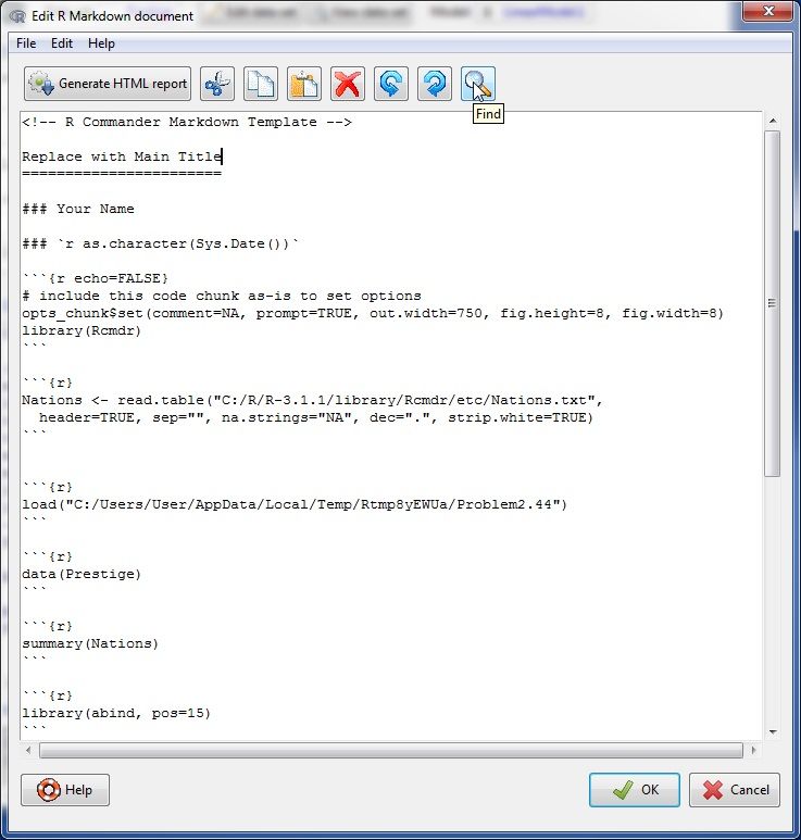
Figure 2: The R Commander window at start-up.

                     3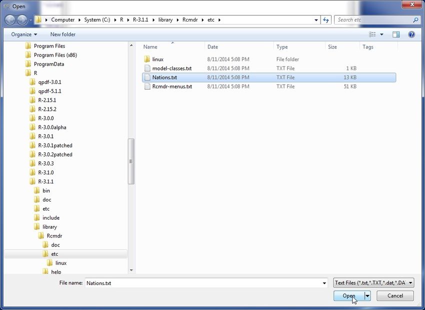
Data Submenus containing menu items for reading and manipulating data.

Statistics Submenus containing menu items for a variety of statistical analyses.
Graphs Menu items for creating various statistical graphs.
Models Menu items and submenus for obtaining numerical summaries, confidence intervals, hypothesis
   tests, diagnostics, and graphs for a statistical model, and for adding diagnostic quantities, such as
   residuals, to the data set.
Distributions Submenus to obtain cumulative probabilities, probability densities or masses, quantiles, and
     graphs of standard statistical distributions (to be used, for example, as a substitute for statistical
     tables), and to generate samples from these distributions.

Tools Menu items for loading R packages unrelated to the Rcmdr package (e.g., to access data saved in
     another package), for loading Rcmdr plug-in packages (see Fox, 2007, Fox and Sá Carvalho, 2012, and
     Section 6.4 below), for setting most R Commander options, and for saving options so that they will
     be applied in subsequent sessions.
Help Menu items to obtain information about the R Commander (including this manual) and associated
    software. As well, each R Commander dialog box has a Help button (see below).

    The complete menu “tree” for the R Commander (version 2.1-0) is shown below. Most menu items
lead to dialog boxes, as illustrated later in this manual. Menu items are inactive (“grayed out”) if they are
inapplicable to the current context. For example, if a data set contains no factors (categorical variables),
the menu items for contingency tables will be inactive.4
File -   Change working directory
    |-   Open script file
    |-   Save script
    |-   Save script as
    |-   Open R Markdown file
    |-   Save R Markdown file
    |-   Save R Markdown file as
    |-   Save output
    |-   Save output as
    |-   Save R workspace
    |-   Save R workspace as
    |-   Exit - from Commander
              |- from Commander and R
Edit -   Edit R Markdown document
    |-   Edit knitr document
    |-   Remove last Markdown command block
    |-   Remove last knitr command block
    |-   Cut
    |-   Copy
    |-   Paste
    |-   Delete
    |-   Find
    |-   Select all
    |-   Undo
    |-   Redo
    |-   Clear Window
   4 Some menu items may not be displayed in certain circumstances. For example, the R Markdown menu items in the File

menu will be displayed only if the R Markdown tab is activated. The menu items shown here are those that are available by
default when the R Commander is running under Windows. The menus also include dividers, which are not shown here,
and menu items leading to dialog boxes are, as is conventional, followed by ..., also not shown.

                                                           4
Data - New data set
    |- Load data set
    |- Merge data sets
    |- Import data - from text file, clipboard, or URL
    |             |- from SPSS data set
    |             |- from SAS xport file
    |             |- from Minitab data set
    |             |- from STATA data set
    |             |- from Excel, Access, or dBase data set [32-bit Windows only]
    |             |- from Excel file [currently 64-bit Windows only]
    |- Data in packages - List data sets in packages
    |                  |- Read data set from attached package
    |- Active data set - Select active data set
    |                 |- Refresh active data set
    |                 |- Help on active data set (if available)
    |                 |- Variables in active data set
    |                 |- Set case names
    |                 |- Subset active data set
    |                 |- Aggregate variables in active data set
    |                 |- Remove row(s) from active data set
    |                 |- Stack variables in active data set
    |                 |- Remove cases with missing data
    |                 |- Save active data set
    |                 |- Export active data set
    |- Manage variables in active data set - Recode variable
                                          |- Compute new variable
                                          |- Add observation numbers to data set
                                          |- Standardize variables
                                          |- Convert numeric variables to factors
                                          |- Bin numeric variable
                                          |- Reorder factor levels
                                          |- Drop unused factor levels
                                          |- Define contrasts for a factor
                                          |- Rename variables
                                          |- Delete variables from data set
Statistics - Summaries - Active data set
          |           |- Numerical summaries
          |           |- Frequency distributions
          |           |- Count missing observations
          |           |- Table of statistics
          |           |- Correlation matrix
          |           |- Correlation test
          |           |- Shapiro-Wilk test of normality
          |- Contingency Tables - Two-way table
          |                    |- Multi-way table
          |                    |- Enter and analyze two-way table
          |- Means - Single-sample t-test
          |       |- Independent-samples t-test
          |       |- Paired t-test
          |       |- One-way ANOVA
          |       |- Multi-way ANOVA
          |- Proportions - Single-sample proportion test
          |             |- Two-sample proportions test
          |- Variances - Two-variances F-test

                                            5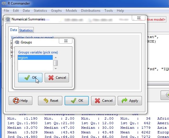
|           |- Bartlett’s test
            |           |- Levene’s test
            |- Nonparametric tests - Two-sample Wilcoxon test
            |                     |- Single-sample Wilcoxon test
            |                     |- Paired-samples Wilcoxon test
            |                     |- Kruskal-Wallis test
            |                     |- Friedman rank-sum test
            |- Dimensional analysis - Scale reliability
            |                      |- Principal-components analysis
            |                      |- Factor analysis
            |                      |- Confirmatory factor analysis
            |                      |- Cluster analysis - k-means cluster analysis
            |                                         |- Hierarchical cluster analysis
            |                                         |- Summarize hierarchical clustering
            |                                         |- Add hierarchical clustering to data set
            |- Fit models - Linear regression
                         |- Linear model
                         |- Generalized linear model
                         |- Multinomial logit model
                         |- Ordinal regression model
Graphs -   Color palette
      |-   Index plot
      |-   Histogram
      |-   Density estimate
      |-   Stem-and-leaf display
      |-   Boxplot
      |-   Quantile-comparison plot
      |-   Scatterplot
      |-   Scatterplot matrix
      |-   Line graph
      |-   XY conditioning plot
      |-   Plot of means
      |-   Strip chart
      |-   Bar graph
      |-   Pie chart
      |-   3D graph - 3D scatterplot
      |            |- Identify observations with mouse
      |            |- Save graph to file
      |-   Save graph to file - as bitmap
                             |- as PDF/Postscript/EPS
                             |- 3D RGL graph
Models -   Select active model
      |-   Summarize model
      |-   Add observation statistics to data
      |-   Confidence intervals
      |-   Akaike Information Criterion (AIC)
      |-   Bayesian Information Criterion (BIC)
      |-   Stepwise model selection
      |-   Subset model selection
      |-   Confidence intervals
      |-   Hypothesis tests - ANOVA table
      |                    |- Compare two models
      |                    |- Linear hypothesis
      |-   Numerical diagnostics - Variance-inflation factors

                                              6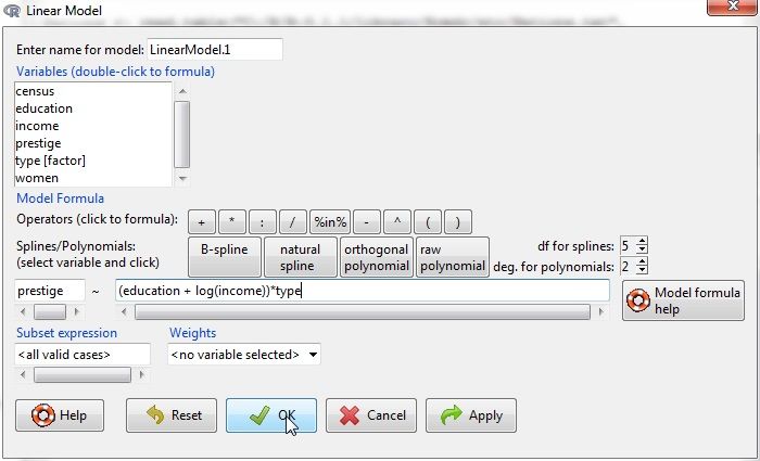
|                        |- Breusch-Pagan test for heteroscedasticity
      |                        |- Durbin-Watson test for autocorrelation
      |                        |- RESET test for nonlinearity
      |                        |- Bonferroni outlier test
      |- Graphs - Basic diagnostic plots
               |- Residual quantile-comparison plot
               |- Component+residual plots
               |- Added-variable plots
               |- Influence plot
               |- Effect plots
Distributions - Continuous distributions - Normal distribution - Normal quantiles
             |            |                      |- Normal probabilities
             |            |                      |- Plot normal distribution
             |            |                      |- Sample from normal distribution
             |            |- t distribution - t quantiles
             |            |                 |- t probabilities
             |            |                 |- Plot t distribution
             |            |                 |- Sample from t distribution
             |            |- Chi-squared distribution - Chi-squared quantiles
             |            |                           |- Chi-squared probabilities
             |            |                           |- Plot chi-squared distribution
             |            |                           |- Sample from chi-squared distribution
             |            |- F distribution - F quantiles
             |            |                 |- F probabilities
             |            |                 |- Plot F distribution
             |            |                 |- Sample from F distribution
             |            |- Exponential distribution - Exponential quantiles
             |            |                           |- Exponential probabilities
             |            |                           |- Plot exponential distribution
             |            |                           |- Sample from exponential distribution
             |            |- Uniform distribution - Uniform quantiles
             |            |                       |- Uniform probabilities
             |            |                       |- Plot uniform distribution
             |            |                       |- Sample from uniform distribution
             |            |- Beta distribution - Beta quantiles
             |            |                    |- Beta probabilities
             |            |                    |- Plot beta distribution
             |            |                    |- Sample from beta distribution
             |            |- Cauchy distribution - Cauchy quantiles
             |            |                      |- Cauchy probabilities
             |            |                      |- Plot Cauchy distribution
             |            |                      |- Sample from Cauchy distribution
             |            |- Logistic distribution - Logistic quantiles
             |            |                        |- Logistic probabilities
             |            |                        |- Plot logistic distribution
             |            |                        |- Sample from logistic distribution
             |            |- Lognormal distribution - Lognormal quantiles
             |            |                         |- Lognormal probabilities
             |            |                         |- Plot lognormal distribution
             |            |                         |- Sample from lognormal distribution
             |            |- Gamma distribution - Gamma quantiles
             |            |                     |- Gamma probabilities
             |            |                     |- Plot gamma distribution
             |            |                     |- Sample from gamma distribution

                                            7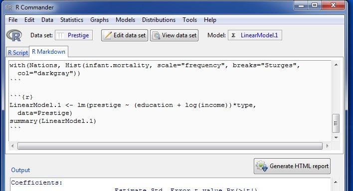
|            |- Weibull distribution - Weibull quantiles
             |            |                      |- Weibull probabilities
             |            |                      |- Sample from Weibull distribution
             |            |- Gumbel distribution - Gumbel quantiles
             |                                  |- Gumbel probabilities
             |                                  |- Plot Gumbel distribution
             |                                  |- Sample from Gumbel distribution
             |- Discrete distributions - Binomial distribution - Binomial quantiles
                          |                       |- Binomial tail probabilities
                          |                       |- Binomial probabilities
                          |                       |- Plot binomial distribution
                          |                       |- Sample from binomial distribution
                          |- Poisson distribution - Poisson quantiles
                          |                     |- Poisson tail probabilities
                          |                     |- Poisson probabilities
                          |                     |- Plot Poisson distribution
                          |                     |- Sample from Poisson distribution
                          |- Geometric distribution - Geometric quantiles
                          |                       |- Geometric tail probabilities
                          |                       |- Geometric probabilities
                          |                       |- Plot geometric distribution
                          |                       |- Sample from geometric distribution
                          |- Hypergeometric distribution - Hypergeometric quantiles
                          |                     |- Hypergeometric tail probabilities
                          |                     |- Hypergeometric probabilities
                          |                     |- Plot hypergeometric distribution
                          |                     |- Sample from hypergeometric distribution
                          |- Negative binomial distribution - Negative binomial quantiles
                                                  |- Negative binomial tail probabilities
                                                  |- Negative binomial probabilities
                                                  |- Plot negative binomial distribution
                                                  |- Sample from negative binomial distribution
Tools - Load package(s)
     |- Load Rcmdr plug-in(s)
     |- Options
     |- Save Rcmdr options
Help - Commander help
    |- Introduction to the R Commander
    |- R Commander website
    |- About Rcmdr
    |- Help on active data set (if available)
    |- Start R help system
    |- R website
    |- Using R Markdown
  The R Commander interface includes a few elements in addition to menus and dialogs:

  • Below the menus is a “toolbar” with a row of buttons.

      – The left-most (flat) button shows the name of the active data set. Initially there is no active data
        set. If you press this button, you will be able to choose among data sets currently in memory (if
        there is more than one). Most of the menus and dialogs in the R Commander reference the
        active data set. (The File, Edit, and Distributions menus are exceptions.)
      – Two buttons allow you to open the R data editor to modify the active data set or a viewer to

                                                    8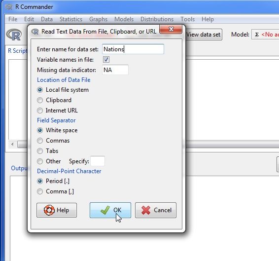
examine it. The data-set viewer can remain open while other operations are performed.5
         – A flat button indicates the name of the active statistical model — a linear model (such as a
           linear-regression model), a generalized linear model, a multinomial logit model, or an ordinal
           regression model.6 Initially there is no active model. If there is more than one model in memory
           associated with the active data set, you can choose among the models by pressing the button.
           The R Commander synchronizes models and the data sets to which they are fit.

    • Immediately below the toolbar is a pane containing the R Script tab, a large scrollable text window.
      As mentioned, commands generated by the R Commander are copied into this window. You can
      edit the text in the Script tab or even type your own R commands into the window. Pressing the
      Submit button, which is at the right below the Script tab (or, alternatively, the key combination Ctrl-
      r,7 for “run,” or Ctrl-Tab), causes the line containing the cursor to be submitted (or resubmitted) for
      execution. If several lines are selected (e.g., by left-clicking and dragging the mouse over them), then
      pressing Submit will cause all of them to be executed. Commands entered into the R Script tab can
      extend over more than one line, but all lines must be submitted simultaneously. The key combination
      Ctrl-a selects all of the text in the Script tab, and Ctrl-s brings up a dialog box to save the contents
      of the tab. The R Markdown tab is described in Section 6.1.
    • Below the R Script and R Markdown tabs is a pane containing a large scrollable and editable text
      window for Output. Commands echoed to the Output pane appear in red, the resulting output in dark
      blue (as in the standard Windows R Console).
    • At the bottom is a small gray pane for Messages. Error messages are displayed in red text, warnings
      in green, and other messages in dark blue. Errors and warnings also provide an audible cue by ringing
      a bell.

    As mentioned, once you have loaded the Rcmdr package, you can minimize the R Console. The R Com-
mander window can also be resized or maximized in the normal manner. If you resize the R Commander,
the width of subsequent R output is automatically adjusted to fit the Output pane.
    The R Commander is highly configurable: We have described the default configuration here. Changes
to the configuration can be made via the Tools −→ Options. . . menu, or — more extensively — by setting
R Commander options in R.8 See Help −→ Commander help for details.

3     Data Input
Most of the procedures in the R Commander assume that there is an active data set.9 If there are several
data sets in memory, you can choose among them, but only one is active. When the R Commander starts
up, there is no active data set.
   The R Commander provides several ways to get data into R:10

    • On platforms other than Mac OS X, you can enter data directly via Data −→ New data set.... This
      is a reasonable choice only for a very small data set.
    • You can import data from a plain-text (“ascii”) file or the clipboard, over the Internet from a URL,
      from another statistical package (Minitab, SPSS, SAS, or Stata), or (under Windows) from an
      Excel, Access, or dBase data set.
   5 The data viewer, provided by the showData function from David Firth’s relimp package (Firth, 2011), can be slow for

data sets with large numbers of variables. When the number of variables exceeds a threshold (initially set to 100), the less
aesthetically pleasing R View command is used instead to display the data set. To use View regardless of the number of variables,
set the threshold to 0. See the R Commander help for details.
   6 R Commander plug-in packages (Fox, 2007; Fox and Carvalho, 2012) may provide additional classes of models.
   7 That is, hold down the Ctrl (or Control) key and simultaneously press the r key.
   8 A menu item that terminates in ellipses (i.e., three dots, ...) leads to a dialog box; this is a standard GUI convention. In

this document, −→ represents selecting a menu item or submenu from a menu.
   9 Procedures selected under via the Distributions menu are exceptions, as is Enter and analyze two-way table... under the

Statistics −→ Contingency tables menu.
  10 Not all of these data sources may be available on all platforms.

                                                               9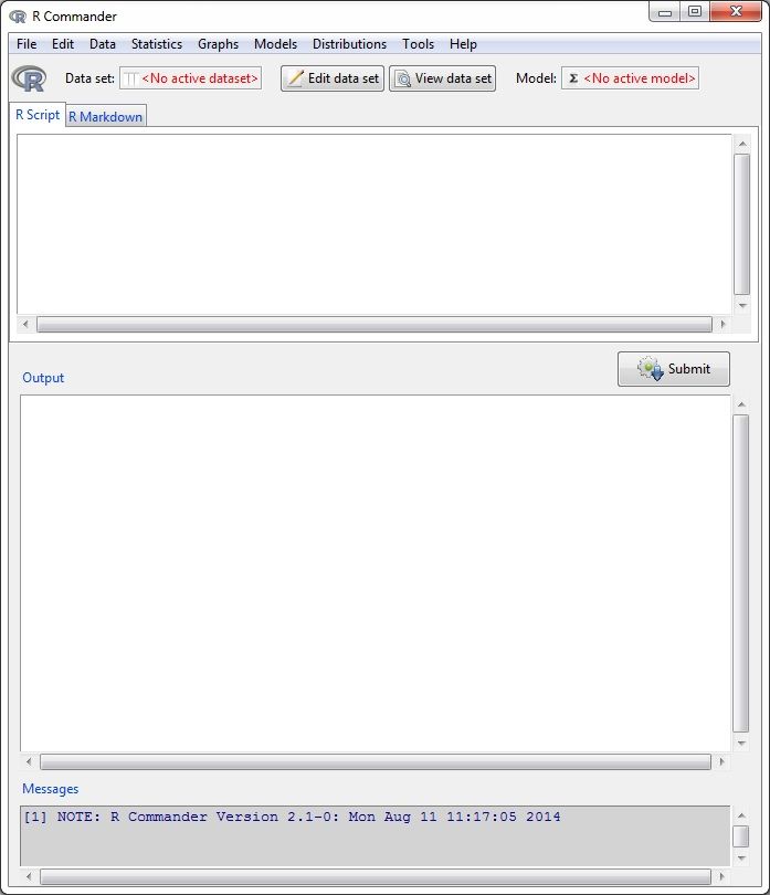
• You can read a data set that is included in an R package, either typing the name of the data set (if
     you know it), or selecting the data set in a dialog box.

3.1    Reading Data From a Text File
For example, consider the data file Nations.txt.11 The first few lines of the file are as follows:
TFR contraception infant.mortality GDP region
Afghanistan                 6.90    NA 154 2848                          Asia
Albania                     2.60    NA   32   863                        Europe
Algeria                     3.81    52   44 1531                         Africa
American-Samoa              NA      NA   11 NA                           Oceania
Andorra                     NA      NA NA    NA                          Europe
Angola                      6.69    NA 124    355                        Africa
Antigua                     NA      53   24 6966                         Americas
Argentina                   2.62    NA   22 8055                         Americas
Armenia                     1.70    22   25   354                        Europe
Australia                   1.89    76    6 20046                        Oceania
. . .

   • The first line of the file contains variable names: TFR (the total fertility rate, expressed as number of
     children per woman), contraception (the rate of contraceptive use among married women, in percent),
     infant.mortality (the infant-mortality rate per 1000 live births), GDP (gross domestic product per
     capita, in U.S. dollars), and region.
   • Subsequent lines contain the data values themselves, one line per country. The data values are separated
     by “white space” — one or more blanks or tabs. Although it is helpful to make the data values line
     up vertically, it is not necessary to do so. Notice that the data lines begin with the country names.
     Because we want these to be the “row names” for the data set, there is no corresponding variable name:
     That is, there are five variable names but six data values on each line, the first of which is alphabetic.
     When this happens, the R read.table command will interpret the first value on each line as the row
     name.
   • Some of the data values are missing. In R, it is most convenient to use NA (representing “not available”)
     to encode missing data, as we have done here.
   • The variables TFR, contraception, infant.mortality, and GDP are numeric (quantitative) variables;
     in contrast, region contains region names. When the data are read, R will treat region as a “factor”
     — that is, as a categorical variable. In most contexts, the R Commander distinguishes between
     numerical variables and factors, and will try to prevent you from doing unreasonable things, such as
     computing the mean of a factor.

   To read the Nations.txt data file into R, select Data −→ Import data −→ from text file, clipboard, or
URL... from the R Commander menus. This operation brings up a Read Text Data dialog, as shown in
Figure 3. The default name of the data set is Dataset. We have changed the name to Nations.
   Valid R names begin with an upper- or lower-case letter (or a period, .) and consist entirely of letters,
periods, underscores ( ), and numerals (i.e., 0–9); in particular, do not include any embedded blanks in a
data-set name. R is case-sensitive, and so, for example, nations, Nations, and NATIONS are distinguished,
and could be used to represent different data sets.
   Clicking the OK button in the Read Text Data dialog brings up an Open file dialog, shown in Figure 4.
Here we navigated to and selected the file Nations.txt. Clicking the Open button in the dialog causes the
data file to be read. Once the data file is read, it becomes the active data set in the R Commander. As a
consequence, in Figure 5, the name of the data set appears in the data set button near the top left of the R
Commander window.
 11 This   file resides in the etc subdirectory of the Rcmdr package. The data are for 1998 and are from the United Nations.

                                                              10
Figure 3: Reading data from a text file.
We next clicked the View data set button to bring up the data viewer window, also shown in Figure
5. The commands to read and view the Nations data set (the R read.table and showData commands)
appear in the R Script tab and Output pane. As well, when the data set is read and becomes the active
data set, a note appears in the Messages pane. The R Commander also issued a library command to
load the relimp package, which was used to display the data set; here, as in general, R packages are loaded
automatically by the R Commander as they are needed.
The read.table command creates an R “data frame,” which is an object containing a rectangular cases-
by-variables data set: The rows of the data set represent cases or observations and the columns represent
variables. Data sets in the R Commander are R data frames.
3.2 Entering Data Directly
If you are using Windows or Linux, you can enter data directly into the R basic spreadsheet-like data
editor.12 A simple alternative, which we in fact prefer, is to save the data in a plain-text file (be careful,
if you create the data file with a word processor, to save it as a plain-text or “ascii” file), typically with
file type .txt, and then to read the file as in the preceding section, via Data −→ Import data −→ from
text file, clipboard, or URL... . If your data are already in a spreadsheet program, such as Excel, you can
simply export the data to a comma-separated-values text file (.csv file), and simply read the file into the R
Commander, being careful to specify the field separator as a comma.
As an example of direct data input, we use a very small data set from Problem 2.44 in Moore (2000):
• Select Data −→ New data set... from the R Commander menus. Optionally enter a name for the data
set, such as Problem2.44, in the resulting dialog box, and click the OK button. (Remember that R
names cannot include embedded blanks.) This will bring up a Data Editor window with an empty
data set.
12 The R data editor for Mac OS X cannot begin with a completely empty data set, and the corresponding menu item
consequently is suppressed.
11Figure 4: Open-file dialog for reading a text data file.
12Figure 5: Displaying the active data set.
• Enter the data from the problem into the first two columns of the data editor. You can move from
one cell to another by using the arrow keys on your keyboard, by tabbing, by pressing the Enter key,
or by pointing with the mouse and left-clicking. When you are finished entering the data, the window
should look like Figure 6.
• Next, click on the name var1 above the first column. This will bring up a Variable editor dialog box,
as in Figure 7.
• Type the variable name age in the box, just as we have, and click the X button at the upper-right corner
of the Variable editor window, or press the Enter key, to close the window. Repeat this procedure to
name the second column height. The Data Editor should now look like Figure 8.
• Select File −→ Close from the Data Editor menus or click the X at the upper-right of the Data Editor
window. The data set that you entered is now the active data set in the R Commander.
3.3 Reading Data from a Package
Many R packages include data. Data sets in packages can be listed in a pop-up window via Data −→ Data
in packages −→ List data sets in packages, and can be read into the R Commander via Data −→ Data in
packages −→ Read data set from an attached package.13 The resulting dialog box is shown in Figure 9. If
you know the name of a data set in a package then you can enter its name directly; otherwise double-clicking
on the name of a package displays its data sets in the right list box; and double-clicking on a data set name
copies the name to the data-set entry field in the dialog.14 Pressing a letter key in the Data set list box will
scroll to the next data set whose name begins with that letter. You can access additional R packages that
are installed in your package library by Tools −→ Load packages.
13 Not all data in packages are data frames, and only data frames are suitable for use in the R Commander. If you try to
read data that are not a data frame, an error message will appear in the messages window.
14 In general in the R Commander, when it is necessary to copy an item from a list box to another location in a dialog, a
double-click is required.
13Figure 6: Data editor after the data are entered.
Figure 7: Dialog box for changing the name of a variable in the data editor.
Figure 8: The Data Editor window after both variable names have been changed.
14Figure 9: Reading data from an attached package — in this case the Prestige data set from the car package.
4 Creating Numerical Summaries and Graphs
Once there is an active data set, you can use the R Commander menus to produce a variety of numerical
summaries and graphs. We will describe just a few basic examples here. A good GUI should be largely
self-explanatory: We hope that once you see how the R Commander works, you will have little trouble
using it, assisted perhaps by the on-line help files.
In the initial examples below, we assume that the active data set is the Nations data set, read from a
text file in the previous section. If you typed in the five-observation data set from Moore (2000), or read in
the Prestige data set from the car package — operations that were also described in the previous section
— then one of these is the active data set. Recall that you can change the active data set by clicking on the
flat button with the active data set’s name near the top left of the R Commander window, choosing from
among a list of data sets currently resident in memory.
Selecting Statistics −→ Summaries −→ Active data set produces the results shown in Figure 10. For
each numerical variable in the data set (TFR, contraception, infant.mortality, and GDP), R reports the
minimum and maximum values, the first and third quartiles, the median, and the mean, along with the
number of missing values. For the categorical variable region, we get the number of observations at each
“level” of the factor. Had the data set included more than ten variables, the R Commander would have
asked us whether we really want to proceed — potentially protecting us from producing unwanted voluminous
output. This menu item is unusual in that it directly invokes an R command rather than leading to a dialog
box, as is more typical of R Commander menus.
For example, selecting Statistics −→ Summaries −→ Numerical summaries... brings up the dialog box
in Figure 11. Only numerical variables appear in the variable list in this dialog; the factor region is excluded
because it is not sensible to compute numerical summaries like the mean and standard deviation for a factor.
We selected the variable infant.mortality by left-clicking on it.15 The Numerical Summaries dialog box
has two tabs: Data and Statistics. Click on the Statistics tab to select it, as shown in Figure 12. In this
case, We’ll take all of the default statistics selections. Clicking OK, produces the following output (in the
Output pane):
> numSummary(Nations[,"infant.mortality"], statistics=c("mean", "sd", "IQR",
+ "quantiles"), quantiles=c(0,.25,.5,.75,1))
mean sd IQR 0% 25% 50% 75% 100% n NA
43.47761 38.75604 54 2 12 30 66 169 201 6
By default, the R command that is executed prints out the mean, standard deviation (sd), and interquartile
range (IQR) of the variable, along with quantiles (percentiles) corresponding to the minimum, the first
15 To select a single variable in a variable-list box, simply left-click on its name. In some contexts, you will have to (or want
to) select more than one variable. In these cases, the usual Windows conventions apply: Left-clicking on a variable selects it
and de-selects any variables that have previously been selected; Shift-left-click extends the selection; and Ctrl-left-click toggles
the selection for an individual variable.
15Figure 10: Getting variable summaries for the active data set.
Figure 11: The Data tab in the Numerical Summaries dialog box.
16Figure 12: The Statistics tab in the Numerical Summaries dialog box.
quartile, the median, the third quartile, and the maximum; n is the number of valid obserations, and NA the
number of missing values.
As is typical of R Commander dialogs, the Numerical Summaries dialog box in Figure 11 includes Help,
Reset, OK, Cancel, and Apply buttons.16 The Help button leads to a help page (which appears in your web
browser) either for the dialog itself or (as here) for an R function that the dialog invokes. The Reset button,
which is present in most R Commander dialogs, resets the dialog to its original state; otherwise, the dialog
retains selections from a previous invocation. Dialog state is also reset when the active data set changes.
As demonstrated, the OK button closes the dialog and generates an R command. The Apply button also
generates a command, but then reopens the dialog in its current state, facilitating the application of several
similar operations. If you make an error in a dialog box — for example, clicking OK without choosing a
variable in the Numerical Summaries dialog — an error message will typically appear and the dialog box
will reopen.
The Numerical Summaries dialog box also makes provision for computing summaries within groups
defined by the levels of a factor. Clicking on the Summarize by groups... button in the Data tab brings up
the Groups dialog, as shown in Figure 13. Because there is only one factor in the Nations data set, only
the variable region appears in the variable list, and it is pre-selected; clicking OK changes the Summarize
by groups... button to Summarize by region (see Figure 14). In this case, we have selected two numerical
variables to summarize, GDP and infant.mortality. Clicking OK produces the following results in the
Output pane:
> numSummary(Nations[,c("GDP", "infant.mortality")], groups=Nations$region,
+ statistics=c("mean", "sd", "IQR", "quantiles"), quantiles=c(0,.25,.5,.75,1))
Variable: GDP
mean sd IQR 0% 25% 50% 75% 100% n NA
Africa 1196.000 2089.614 795.50 36 209.00 389.5 1004.50 11854 54 1
Americas 5398.000 6083.311 5268.50 386 1749.25 2765.5 7017.75 26037 40 1
Asia 4505.051 6277.738 6062.50 122 345.00 1079.0 6407.50 22898 39 2
Europe 13698.909 13165.412 24582.25 271 1643.75 9222.5 26226.00 42416 44 1
Oceania 8732.600 11328.708 16409.25 654 1102.75 2348.5 17512.00 41718 20 5
Variable: infant.mortality
mean sd IQR 0% 25% 50% 75% 100% n NA
Africa 85.27273 35.188095 50.0 7 61.00 85.0 111.00 169 55 0
16 The order of the buttons varies according to the operating system, and is different, for example, in Mac OS X than in
Windows.
17Figure 13: Selecting a grouping variable in the Groups dialog box.
Figure 14: The Numerical Summaries dialog box after the grouping variable region has been chosen and
with two numeric variables selected.
18Figure 15: The Histogram dialog.
Americas 25.60000 17.439713 24.0 6 12.00 21.5 36.00 82 40 1
Asia 45.65854 32.980001 50.0 5 22.00 37.0 72.00 154 41 0
Europe 11.85366 7.122363 10.0 5 6.00 8.0 16.00 32 41 4
Oceania 27.79167 29.622229 26.5 2 9.25 20.0 35.75 135 24 1
Several other R Commander dialogs allow you to select a grouping variable in this manner.
Making graphs with the R Commander is also straightforward. For example, selecting Graphs −→
Histogram... from the R Commander menus produces the Histogram dialog box in Figure 15. There are
Data and Options tabs in this dialog. We’ll take all the default options (the Options tab isn’t shown), and
clicking on infant.mortality followed by OK, opens a Graphics Device window with the histogram shown
in Figure 16. If you make several graphs in a session, then only the most recent normally appears in the
Graphics Device window.17
5 Statistical Models
Several kinds of statistical models can be fit in the R Commander using menu items under Statistics
−→ Fit models: linear models (by both Linear regression and Linear model ), generalized linear models,
multinomial logit models, and ordinal regression models such as the proportional-odds model [the latter two
from Venables and Ripley’s nnet and MASS packages, respectively (Venables and Ripley, 2002)]. Although
the resulting dialog boxes differ in certain details (for example, the generalized linear model dialog makes
provision for selecting a distributional family and corresponding link function), they share a common general
structure, as illustrated in the Linear Model dialog in Figure 17.18 Before selecting Statistics −→ Fit models
−→ Linear Model, we made Prestige the active data set by clicking on the active data set button and
selecting Prestige from the resulting list. Recall that the Prestige data were read from the car package
in Section 3.3.
• Double-clicking on a variable in the variable-list box copies it to the model formula — to the left-hand
side of the formula, if it is empty, otherwise to the right-hand side (with a preceding + sign if the
context requires it). Note that factors (categorical variables) are parenthetically labelled as such in
the variable list.19 Entering a factor into the right-hand side of a statistical model formula generates
dummy-variable regressors.
17 On Windows, you can recall previous graphs using the Page Up and Page Down keys on your keyboard if you first turn
on the graph history feature of the Windows R graphics device, via History −→ Recording. This feature is available only on
Windows systems. Dynamic three-dimensional scatterplots created by Graphs −→ 3D graph −→ 3D scatterplot... appear in
a special RGL device window; likewise, effect displays created for statistical models (Fox, 2003; Fox and Hong, 2009) via Models
−→ Graphs −→ Effect plots appear in individual graphics-device windows.
18 An exception is the Linear Regression dialog in which the response variable and explanatory variables are simply selected
by name from list boxes containing the numeric variables in the current data set.
19 Some data frames contain logical variables (with values TRUE and FALSE) and character variables, with values that are text
strings (such as "male" and "female"). If such variables are present, the R Commander will treat them as if they were factors.
19Figure 16: A graphics window containing the histogram for infant mortality in the Nations data set.
Figure 17: The Linear Model dialog box, with Prestige from the car package as the active data set.
20• The top row of buttons in the toolbar above the formula can be used to enter operators and parentheses
into the right-hand side of the formula.
• The bottom row of buttons in the toolbar can be conveniently used to enter regression-spline and
polynomial terms into the model formula, with the degrees of freedom for splines and the degree of
polynomials controlled by the spin-boxes to the right of the buttons (defaulting to 5 df and degree 2,
respectively).
• You can also type directly into the formula fields, and indeed may have to do so, for example, to put
a term such as log(income) into the formula, as we’ve done here. Some information on R model
formulas may be obtained by pressing the Model formula help button in the linear-model dialog.
• The name of the model, here LinearModel.1, is automatically generated, but you can substitute any
valid R name.
• You can type an R expression into the box labelled Subset expression; if supplied, this is passed to the
subset argument of the lm function, and is used to fit the model to a subset of the observations in
the data set. One form of subset expression is a logical expression that evaluates to TRUE or FALSE for
each observation, such as type != "prof" (which would select all non-professional occupations from
the Prestige data set).
• Optionally selecting a weight variable in the Weights drop-down list produces a weight-least-squares
(WLS) regression.
Clicking the OK button generates the following command and output, and makes LinearModel.1 the
active model, with its name displayed in the Model button:
> LinearModel.1 summary(LinearModel.1)
Call:
lm(formula = prestige ~ (education + log(income)) * type, data = Prestige)
Residuals:
Min 1Q Median 3Q Max
-13.970 -4.124 1.206 3.829 18.059
Coefficients:
Estimate Std. Error t value Pr(>|t|)
(Intercept) -120.0459 20.1576 -5.955 5.07e-08 ***
education 2.3357 0.9277 2.518 0.01360 *
log(income) 15.9825 2.6059 6.133 2.32e-08 ***
type[T.prof] 85.1601 31.1810 2.731 0.00761 **
type[T.wc] 30.2412 37.9788 0.796 0.42800
education:type[T.prof] 0.6974 1.2895 0.541 0.58998
education:type[T.wc] 3.6400 1.7589 2.069 0.04140 *
log(income):type[T.prof] -9.4288 3.7751 -2.498 0.01434 *
log(income):type[T.wc] -8.1556 4.4029 -1.852 0.06730 .
---
Signif. codes: 0 ’***’ 0.001 ’**’ 0.01 ’*’ 0.05 ’.’ 0.1 ’ ’ 1
Residual standard error: 6.409 on 89 degrees of freedom
In most context, this will work properly. Note character data read from plain-text files will automatically be converted to
factors.
21(4 observations deleted due to missingness)
Multiple R-squared: 0.871, Adjusted R-squared: 0.8595
F-statistic: 75.15 on 8 and 89 DF, p-value: < 2.2e-16
Operations on the active model may be selected from the Models menu. For example, Models −→
Hypothesis tests −→ Anova table..., followed by selecting the default “Type-II” tests, produces the following
output:
> Anova(LinearModel.1, type="II")
Anova Table (Type II tests)
Response: prestige
Sum Sq Df F value Pr(>F)
education 1209.3 1 29.4446 4.912e-07 ***
log(income) 1690.8 1 41.1670 6.589e-09 ***
type 469.1 2 5.7103 0.004642 **
education:type 178.8 2 2.1762 0.119474
log(income):type 290.3 2 3.5344 0.033338 *
Residuals 3655.4 89
---
Signif. codes: 0 ’***’ 0.001 ’**’ 0.01 ’*’ 0.05 ’.’ 0.1 ’ ’ 1
6 Odds and Ends
6.1 Producing Reports
In its default configuration, the R Commander includes an R Markdown tab in the upper pane, which
accumulates the commands generated during the session in an R Markdown document.20 Figure 18 shows
the R Markdown tab for the current session, which we’ve scrolled to the top of the generated document. As
its name implies, R Markdown is a simple markup language, which includes blocks of R commands, and
can be used to generate HTML (i.e., web) pages. For more information about R Markdown, select Help
−→ Using R Markdown from the R Commander menus.21
Each set of commands generated by the R Commander produces a block of R commands in the R
Markdown document.22 These blocks are delimited by ‘‘‘{r} at the start of each block and by ‘‘‘ (three
back-ticks) at the end of the block. Even if you are unfamiliar with R commands, you can see the relationship
between commands and resulting output in the Output pane.
The R Markdown tab is editable, and so you can modify and add to the text in the tab. It is generally
safe to type whatever explanatory text you wish between blocks of R code (see below). In general, however,
unless you know what you’re doing, you should not modify R code blocks in the R Markdown document
or add your own code blocks. You can, however, remove entire blocks of code, as long as subsequent blocks
don’t depend on them — and you will likely want to remove command blocks that produce unwanted output.
Command blocks that produce errors are removed automatically. You can remove the most recent command
block by selecting Remove last Markdown Command Block from the Edit menu, or by right-clicking in the
R Markdown tab and selecting Remove last Markdown Command Block from the context menu. The first
code block (which begins ‘‘‘{r echo=FALSE}) sets some options for the software from the knitr package
(Xie, 2013) that is used to process the R Markdown text, and this block should not normally be modified.
With some lines elided (indicated by . . .), here is the R Markdown document produced for the
current session:
20 The R Commander can also optionally create a knitr LaTeX document (Xie, 2013) and compile it into a PDF file.
This option requires a LaTeX installation, and is activated by the setting the Rcmdr option use.knitr to TRUE. see Help −→
Commander help and Tools −→ Options.
21 This and some other items in the Help menu require an active Internet connection.
22 Commands that require direct user interaction, such as interactive point identification in a graph, are suppressed in the R
Markdown document. As well, commands that generate errors are removed from the document.
22Figure 18: The R Markdown tab, with Generate HTML report button.
Replace with Main Title
=======================
### Your Name
### ‘r as.character(Sys.Date())‘
"‘{r echo=FALSE}
# include this code chunk as-is to set options
opts_chunk$set(comment=NA, prompt=TRUE, out.width=750, fig.height=8, fig.width=8)
library(Rcmdr)
"‘
"‘{r}
Nationsdata=Prestige)
summary(LinearModel.1)
"‘
"‘{r}
Anova(LinearModel.1, type="II")
"‘
It is probably unnecessary to explain that you would normally replace “Your Name” with your name, and
replace “Replace with Main Title” with the title of the report that you want to create. Perhaps less
obviously, you can type arbitrary explanatory text before the first command block, in between R code blocks
— that is, between the terminating ‘‘‘ of one block and starting ‘‘‘{r} of the next — and after the last
command block. You can take advantage of the simple markup provided by R Markdown; for example, text
enclosed in asterisks (e.g., *this is important*) will be set in italic type. To illustrate, we added the text
“Let us regress occupational prestige ... ” immediately before the R command block performing
the regression.
Once you have finished editing the R Markdown document, you can generate an HTML page from it
by pressing the Generate HTML report button below the R Markdown tab. The report should open in your
web browser. The R Markdown document can be saved via the File menu.
You can also open a separate, larger editor window to edit the R Markdown document (see Figure 19):
Select Edit R Markdown document from the R Commander Edit menu; right-click in the R Markdown tab
and select Edit R Markdown document from the context menu; or press the key-combination Control-E when
the cursor is in the R Markdown tab. The editor supports the usual Edit-menu and right-click context-menu
commands, and also allows you to compile the R Markdown document into an HTML report. Clicking the
OK button in the editor saves your edits to the R Markdown tab, and clicking Cancel discards your edits.
Below the menu in the editor, there is a largely self-explanatory toolbar with various buttons; if you hover
the mouse over a button, a “tool-tip” will display.
6.2 Saving and Printing Output
You can also save text output directly from the File menu in the R Commander; likewise you can save or
print a graph from the File menu in an R Graphics Device window. If you prefer not to use the R Markdown
tab, you can collect the text output and graphs that you want to keep in a word-processor document. In this
manner, you can intersperse R output with your typed notes and explanations. This procedure, however,
has the disadvantage that it is not directly reproducible, while an R Markdown document can subsequently
be executed to reproduce your analysis, possibly with modifications.
Open a word processor such as Word, OpenOffice Writer, or even Windows WordPad. To copy
text from the Output pane, block the text with the mouse, select Copy from the Edit menu (or press the key
combination Ctrl-c, or right-click in the pane and select Copy from the context menu), and then paste the text
into the word-processor document via Edit −→ Paste (or Ctrl-v or right-click Paste), as you would for any
Windows application. One point worth mentioning is that you should use a monospaced (“typewriter”)
font, such as Courier New, for text output from R; otherwise the output will not line up neatly.
Likewise, to copy a graph, select File −→ Copy to the clipboard −→ as a Metafile from the R Graphics
Device menus; then paste the graph into the word-processor document via Edit −→ Paste (or Ctrl-v or
right-click Paste). Alternatively, you can use Ctrl-w to copy the graph from the R Graphics Device, or
right-click on the graph to bring up a context menu, from which you can select Copy as metafile.23 At the
end of your R session, you can save or print the document that you have created, providing an annotated
record of your work.
Alternative routes to saving text and graphical output may be found respectively under the R Com-
mander File and Graphs −→ Save graph to file menus. Saving the R Commander Script tab, via File
−→ Save script, allows you to reproduce your work on a future occasion.
23 As you will see when you examine these menus, you can save graphs in a variety of formats, and to files as well as to the
clipboard. The procedure suggested here is straightforward, however, and generally results in high-quality graphs. Once again,
this description applies to Windows systems.
24Figure 19: The R Markdown document editor.
256.3 Entering Commands in the Script Tab
The R Script tab provides a simple facility for editing, entering, and executing commands. Commands
generated by the R Commander appear in the Script tab, and you can type and edit commands in the
tab more or less as in any editor. The R Commander does not provide a true “console” for R, however,
and the Script tab has some limitations. For example, all lines of a multiline command must be submitted
simultaneously for execution. For serious R programming, it is preferable to use the script editors provided
by the Windows and Mac OS X versions of R, or — even better — a programming editor or interactive
development environment, such as RStudio .24
6.4 Using R Commander Plug-ins
R Commander plug-ins are R packages that add to the capabilities of the R Commander. Many such
plug-ins are currently available on CRAN, and may be downloaded and installed in the normal manner.
Plug-ins typically add menus or menu items and associated dialog boxes to the R Commander. They may
also modify or remove existing menu items or dialogs. A properly programmed R Commander plug-in can
be loaded either directly, in which case the R Commander loads along with the plug-in, or from the R
Commander via Tools −→ Load Rcmdr plug-in(s)... . In the latter event, the R Commander will restart
to activate the plug-in. It is possible to use several plug-ins simultaneously, but plug-ins may also conflict
with each other. For example, one plug-in may remove a menu to which another plug-in tries to add a menu
item.
6.5 Terminating the R Session
There are several ways to terminate your session. For example, you can select File −→ Exit −→ From
Commander and R from the R Commander menus. You will be asked to confirm, and then asked whether
you want to save the contents of the R Script, Output, and R Markdow n windows. Likewise, you can select
File −→ Exit from the R Console; in this case, you will be asked whether you want to save the R workspace
(i.e., the data that R keeps in memory); you would normally answer No.
References
Firth, D. (2011). relimp: Relative Contribution of Effects in a Regression Model. R package version 1.0-3.
Fox, J. (2003). Effect displays in R for generalised linear models. Journal of Statistical Software, 8(15):1–27.
Fox, J. (2005). The R Commander: A basic-statistics graphical user interface to R. Journal of Statistical
Software, 19(9):1–42.
Fox, J. (2007). Extending the R Commander by “plug-in” packages. R News, 7(3):46–52.
Fox, J. and Hong, J. (2009). Effect displays in R for multinomial and proportional-odds logit models:
Extensions to the effects package. Journal of Statistical Software, 32(1):1–24.
Fox, J. and Sá Carvalho, M. (2012). The RcmdrPlugin.survival package: Extending the R Commander to
survival analysis. Journal of Statistical Software, 49(7):1–32.
Moore, D. S. (2000). The Basic Practice of Statistics. Freeman, New York, second edition.
R Core Team (2014). R: A Language and Environment for Statistical Computing. R Foundation for Statistical
Computing, Vienna, Austria.
Venables, W. N. and Ripley, B. D. (2002). Modern Applied Statistics with S. Springer, New York, fourth
edition. ISBN 0-387-95457-0.
Xie, Y. (2013). knitr: A general-purpose package for dynamic report generation in R. R package version 1.2.
24 The R Commander will run under RStudio, in which case by default R Commander output and messages are directed
to the R console within RStudio, but there are some issues, such as partial incompatibility with the RStudio Plot and Help
tabs.
26You can also read