Digital Data Viewer - User's Manual Version 0.57 June 20, 2006
←
→
Page content transcription
If your browser does not render page correctly, please read the page content below
Digital

  Data

     Viewer
     User’s Manual

           Version 0.57
          June 20, 2006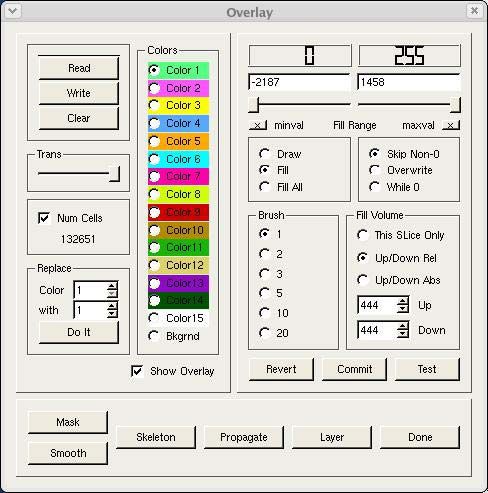
Table of Contents
I. Introduction                                1
II. Input and Output File Types               1
III. Starting DDV                              3
IV. Mouse Functions                            5
V. Other Main Window Functions                 5
VI. Effects of Operations on Internal Data     7
VII. Histogram Window                          8
VIII. Data Repair                             11
IX. Fill                                      12
X. Overlay Widget                             13
XI. Isosurface                                16
XII. Two-D Plots                              18
XIII. One-D Plots                             19
XIV. Fiducial Registration                    20
XV. Medial Axis (Skeleton)                    21
XVI. Python Widget                            21
XVII. Data Operations Widget                  22

Appendix A. Data Formats                      25

Appendix B. For Mac Users                     26

                                                   i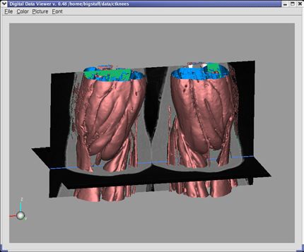
I. Introduction

DDV lets you view and edit stacks of slices of image data and create three dimensional
surfaces from these images. It is written in C++ and uses industry-standard libraries,
including Qt for the graphical user interface and OpenGL for graphics. Binary versions
are available for the following platforms:

       •   Linux
       •   64 bit Linux
       •   Microsoft Windows
       •   Apple Macintosh MacOSX 10.3 (Mac Users, please read Appendix B.)

These, along with this manual in pdf format, can be downloaded from the Web site
www.compgeomco.com .

There is an email list for receiving information on upgrades and bug fixes. To get on the
list, send email to john@compgeomco.com asking to be included.

DDV is currently under development. You are encouraged to submit suggestions and
requests for improvement, as well as bug reports, to the above email address.

Because of the lack of standardization with regard to graphics drivers on the Linux OS,
DDV might fail to execute on this system. If you have problems, please let us know.
The current version of DDV expects some kind of hardware graphics acceleration to be
available. Thanks to the video gaming market, hardware accelerated graphics boards
have become inexpensive commodity items; we recommend that you purchase one and
install the appropriate drivers, if necessary.

II. Input and Output File Types
DDV currently accepts four types of file for input: TIFF, plain data, various OTHER
types, and its own format ( Appendix A). TIFF or OTHER files contain one slice of
image data per file. Each TIFF or OTHER file is assumed to contain an XY slice of
image data. The TIFF format can be any of the following:

                                                                                          1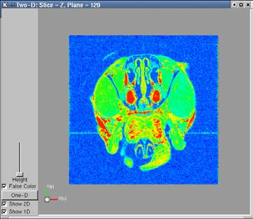
•   1-bit black and white
   •   8-bit grey scale
   •   24-bit RGB color

For 24-bit color TIFFs, DDV will sum the three components and present the data on a
grey scale going from black (minimum value in file) to white (maximum value in file).
You can change the relative red, green, and blue channel intensities on the left side of the
TIFF file browser (see below). The algorithm for computing the final grayscale value is:

    Intensity = (ri*rv + gi*gv + bi*bv)/(ri + gi + gv)

where the i’s refer to the relative intensities from the browser and the v’s are the actual
data values in the file. The default is equal values for all of the the i’s. After the TIFF or
OTHER files have been read, you will see a widget that lets you set the element spacing
in x, y, and z. The default is 1.0 for each direction.

DDV will not show any images in colors other than grey, except for the false color option
in 2-D windows, described later.

The plain data format is any ASCII file that contains data written from a triple-nested
loop like this:

  for ( z = 0; z < zmax; z++ ) {
    for ( y = 0; y < ymax; y++ ) {
        for ( x = 0; x < xmax; x++ ) {
           (ASCII_write(data(x,y,z));
        }
    }
  }

You will be prompted to supply the values of xmax, ymax, and zmax, and the type of
data. DDV doesn’t check whether the data will actually fit in the type that you specify
(e.g. specifying unsigned byte but having a data value of less than zero or greater than
255). If the values of xmax, ymax, and zmax that you specify are incorrect, the resulting
images in DDV will look strange.

You can write the three dimensional data from DDV only in its native format. To do this,
see “Section V: Other Main Window Functions”, below. You can also write overlay and
isosurface data from DDV. These will be described in later sections of this manual. Any
of the windows that display images of the data (Main, 2-D, or 1-D) provide for the
creation of image files of the window’s contents by selecting the “File” pulldown for that
window.

                                                                                             2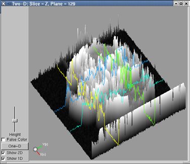
III. Starting DDV
On Unix or Linux systems, typing the command “ddv” will bring up the Intro Dialog
shown here. On Windows or MacOSX, you can click on the DDV icon.

                     After selecting the type of file that you want to read, the main file
                     browser appears if you are reading a DDV file. If you are reading
                     TIFF or OTHER files, a slightly different browser appears that will
                     let you change the relative red, green, and blue channel intensities
                     on the left side of the browser. The TIFF browser is shown here
                     with a group of files selected (highlighted).

To select multiple TIFF or OTHER files, left-click on the first file in the sequence, then
SHIFT-left click on the last file. Selecting multiple files with the File Browser can be
tedious, so it is recommended that, after selecting a set of TIFF files, you write out the
data using DDV’s format using the File->Write All pulldown from the main window.
Then next time you will have to click on just one file.

The list of files from the File Browser will be sorted in lexical order to determine the
sequence for reading, regardless of the order in which they are selected in the browser.
Thus, the following list of files: 1tiff 2tiff 3tiff … 10tiff 11tiff … would be read in as:
1tiff 10tiff 11tiff … 2tiff 20tiff 21tiff … 3tiff … , which is probably not what was
intended. The current solution to this problem is to name your TIFF files like this:
0001tiff 0002tiff 0003tiff … , or in some similar format.

The ITK option lets you read a file from the Insight Segmentation and Registration
Toolkit www.itk.org . The .mha format text file is expected. Only 3-D, 8-bit data will be
accepted.

After you have selected the file(s) for input, the message “Loading …” will appear in the
Intro Dialog in place of the file-type pushbuttons.

                                                                                              3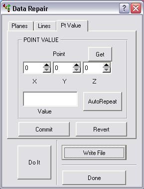
One or more Progress Bars might appear.

After the input data have been read, the Intro Dialog will disappear and you will see the
Main Window and the Geometry Window. The Main Window will initially display the
x-y slice at a z value halfway through the data set.

                                           To view slices perpendicular to the X, Y, or Z
                                           direction, click on the appropriate check
                                           box(es) and move the slider(s). Alternatively,
                                           you can type into the spin box below each
                                           slider or use the up/down indicators. Clicking
                                           on a slider widget above or below the handle
                                           will cause the slider to increment or decrement
                                           by one unit. This should be true for any of
                                           DDV’s sliders. (The Python button will not
                                           appear on Windows versions of DDV.)

                                                                                            4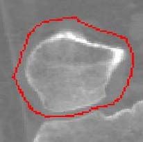
The Clip Slider section of the Geometry Window lets you select a subset of the viewable
images. You might want to do this if you are going to work on just a small portion of the
data or if your graphics hardware is slow in drawing the full images. Also, note that
many of the functions to be discussed later will operate only on the selected subset of the
data. The numbers in the spin boxes under the clip sliders show the range of values in X,
Y, and Z. Subset selection can be manipulated using the spin boxes as well as with the
sliders.

IV. Mouse Functions
You use the mouse to rotate, translate, or scale the image in the viewing area of the Main
Window, as shown below.

   •   Left Button: rotation
   •   Middle Button: translation (panning)
   •   Right Button: scaling (zooming – moving up zooms in)

You can rotate the image by pressing and holding the left mouse button and dragging the
image in the desired rotation direction. It should be fairly intuitive. Additionally, you
can rotate the image around an axis coming out of the center of the screen by positioning
the mouse near the edge of the viewing area and clicking and dragging in a circular arc in
the desired direction of rotation.

                                                 (b)
                            (a)

                                  rotate
                                  in direction
                                  of drag
                     CENTER OF
                     ROTATION

                             rotate about axis coming out
                             from center of screen

If you have a two button mouse, emulation of the middle button might be provided by
pressing both buttons simultaneously. This is system-dependent.

To make it easier to go from slice to slice when performing repetitive operations, such as
segmentation or registration, you can increment any slice that is visible by holding the
Shift key and pressing the Middle Mouse button. You can decrement the slice plane by
holding Shift and pressing the Right Mouse button.

V. Other Main Window Functions
Below the Main Window Title Bar, there are four pull down menus. Each pull down
function also has a keyboard accelerator. The keyboard accelerators let you perform the

                                                                                          5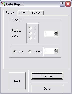
same function by pressing the Control (CTRL) key and holding it
while pressing another key specific to the operation. This works
only if the mouse focus is in the Main Window, usually attained
by clicking the mouse button while the pointer is in the Main
Window.
The File pulldown lets you exit DDV by selecting “Exit” from the
pulldown or by entering CRTL-Q. You can also write files in DDV format or an image
file of the Main Window contents. The options are:
o Write all – Writes a DDV file containing the entire dataset.
o Write subset – Writes a DDV file containing just the data that remains after the
Geometry Window clip sliders have been applied.
o Write lowres – Writes a DDV file with one quarter of the resolution in x and y
but full resolution in z. In future versions, this option will be more flexible.
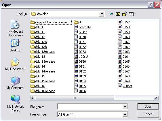
o Write image – Writes an image file of the contents of the Main Window. After
selecting this option, the File Browser Dialog below appears. You may select an
image format before creating the
file. The number and names of
image formats may be system
independent. The name of the file
that you create will have the image
format appended to it in lower case
with a separating dot. Axis labels
will not appear in the image. This
bug will be fixed when I figure out
how to do it.
o Write temp – Writes a temporary
file containing the DDV data array. This file is accessible only through the Read
temp pulldown and will not persist past the end of the program.
o Write ITK – Writes a .mha and a .raw file for reading into ITK. Only 8-bit data
is supported.
o Read temp – Reads the temporary DDV data back into the program.
The Color pulldown lets you select a color for the background of all windows open by
the current application. This is useful in a situation where you have more than one
instance of DDV running simultaneously, so that you can easily see which windows go
with which instance of the application. You can change the window background by
selecting one of the five colors at any time.
The Picture pulldown offers the following selections:
Clicking on the “contrast (CRL-G)” selection causes this slider to
appear:
6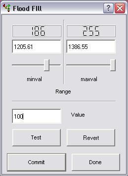
The Contrast slider lets you adjust the overall brightness of the image by
               adjusting the grey scale-to-brightness conversion table. The apparent
               brightness of mid-grey scale data varies from system to system and
               monitor to monitor. Think of it as a contrast adjustment for the monitor.
               It has no effect on the data values that underlie the image. Moving the
               slider up makes mid-grey values brighter.

“toggle stride (CTRL-T)” causes only every third visible data element to be drawn when
the mouse is moving. This is useful if your system has slow graphics or you are looking
at a huge data set. This feature affects isosurface drawing in a similar manner. When
toggled on, the graphics is about a factor of ten more responsive during mouse
movement.

The “reset (CTRL-R)” selection is useful after subsetting the image with the Clip Sliders
in the Geometry Window or using “subset” to recenter the visible range of data. It also
moves the center of rotation to the center of the visible range.

“subset (CTRL-S)” can be used to quickly select a range portion of the image for
clipping. After selecting “subset” you are required to select two points on the image in
the drawing area. After doing this, the viewable portion of the image data will be clipped
to fall within the rectangle that you just selected and the sliders and spin boxes in the
Geometry Window will be appropriately updated. If you later want to increase the size of
the clipped region, use the Geometry Window Clip Sliders.

“toggle axes (CTRL-A)” turns the axes in the main window and any existing two-d
windows on or off.

“toggle Blue” controls visibility of the blue line that appears at the intersection where
more than one slice plane is visible.

The “Font” pulldown brings up a Font Selector Widget that lets you change the font,
style, and size for all of the widgets in DDV. This is useful if the fonts are too big to
show the entire label on a pushbutton, for instance.

VI. Effects of Operations on Internal Data
DDV has several types of internal data. If will be useful to be aware of these and how the
various functions affect them.

   o   Real Data
   o   Slice Data
   o   Overlay Data
   o   Isosurface Data

                                                                                            7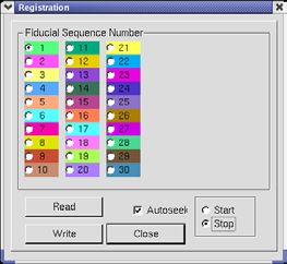
The term “real data” refers to the internal representation that DDV maintains of the data
as read in from the slices or from its own format. This data is queried by the slice and
overlay data and can be modified by several operations:

   o Data Repair
   o Histogram
   o Fill

Slice data consist of the planes that are currently seleced for viewing. Every time that a
new slice plane is selected, the slice data for that plane are reconstructed from the real
data. Slice data can be modified by:

   o Selecting a new slice
   o Histogram
   o Otherwise modifying data on a currently visible slice

Overlay data are kept in a separate data array, each element of which corresponds to an
element in the real data. Overlay data are used for copying data from the real data by
filling or by drawing onto the overlay slices. You can find more explanation below in the
section on overlay data. Overlay data are not affected by Data Repair, Histogram, or Fill
operations.

Isosurface data are triangles that form a surface of constant value for either real or
overlay data.

VII. Histogram Window
When DDV reads in a data set, whether from slices or from its own format, it creates a
histogram of intensity values for the data. You can see the Histogram Window by
clicking on the Histogram button in the Geometry Window. An example is below.

                                                                                             8
(a) (b)
Histogram Example. (a) Original histogram; (b) after selection of a portion; (c) after
“Apply”; (d) “Apply” options
(d)
(c)
Figure (a) shows the histogram of the original
data set. In Fig. (b) we used the Zoom+ button to increase the height of the histogram
and the Select button to identify a portion of the histogram for expansion. Clicking on
“Select” causes the cursor to change to the “+” cursor and the data value will appear next
to the cursor. You then drag the mouse in the Histogram Window while holding down
the left button to select a part of the histogram. At any time before clicking “Apply” you
can select “Reset” to revert to the previous histogram. To exit from Select mode, either
click “Apply” or click “Select” again.
If you click “Apply”, the Apply options panel shown in Fig. (d) appears. This lets you
control the data values outside the selected range. The default is to set those below the
range to the data minimum and those above to the data maximum value. When you
select “OK”, the selected part of the histogram is expanded to fill the grey scale range of
values. This affects only the Slice Data unless you subsequently select the “->toData”
button. Then you will be reminded that continuing will alter the Real Data by applying
the histogram change to it. If you select “Accept” from the dialog that appears, the Real
Data will be changed in the same way as the Slice Data. The only way to go back after
this is to restart DDV and read in the data again.
Here are the “before” and “after” effects of the histogram operations that were shown
above. Figure (c) shows the result of selecting the “Above Range” values to become the
minimum value.
9(a) (b) (c)
Slice image before histogram alteration (a), after (b), and after setting “Above Range”
values to minumin (c);
Altering the histogram provides a way of highlighting subtle changes in the data values.
Remember that changes to the histogram alter only the Slice Data unless the change is
specifically made to the Real Data by pressing the “->toData” button. After this step,
they are irreversible.
With version 0.40 of DDV, the histogram widget gained a button labeled “Mask” which,
if clicked, will bring up the Histogram Mask widget, shown here. With it you can choose
from among several curves that will let you modify element values according to the curve
chosen. As with the main Histogram widget, any choices you make will only affect the
visual appearance, leaving the real data unchanged unless you click on the ->toData
button, after which the changes will be irreversible. The following icon buttons are
available:
(a) Ramp: Clicking on this button causes each element in a given histogram
bin to be replaced by its current value, which leaves them unchanged. It is
useful for resetting the histogram to its original state (assuming that you have
not clicked on ->toData).
(b) Inverse Ramp: This button replaces each element value by the maximum
data value minus the current data value. This has the effect of inverting the
image intensities, so that for instance black becomes white and white becomes
black.
(c) Gamma Ramp: Clicking on this button and then moving the slider on the
right side of the widget will change the relative contrast of the elements,
making the image brighter or darker while maintaining the extreme data
values.
(d) Gaussian: The first time you click on this button you will see a message
window that tells how to use it. You have to click “OK” to make the message window
go away, then click on the place in the histogram where you want the center of the
Gaussian distribution to occur. Then use the slider to change the width. This has the
effect of making the elements in histogram bins nearest to the center have high intensities
while elements in bins farther from the center will have intensities that fall off to black.
This feature is probably not very useful, but I coded it and you can try it if you want to.
(e) Step: The first time you click on this button you will see a message window that tells
how to use it. You have to click “OK” to make the message window go away, then click
10twice on the histogram to specify the left and right edges of the step. This will have the
effect of making all of the elements in bins inside the step become white, and all other
elements become black.
(f) Modified Ramp: This works like Step, but has the effect only of setting elements
outside the ramp to black.
(g) ->toData: Clicking this button will bring up a message box reminding you that this
change will be irreversible. If you click “Accept”, the real data will be irreversibly
altered and a new histogram will be computed.
VIII. Data Repair
To bring up the Data Repair Widget, click on “Data Repair” in the
Geometry Window.
You can use the Data Repair Widget to write out a data file in DDV
format. Do this by selecting “Write File”, at which point you will be
prompted for a file name. The other uses of Data Repair have a direct
effect on the Real Data. You can replace a slice of data with another
slice or with the average of the two surrounding slices; similarly, you
can replace a line of data that consists of the intersection of two slices
with another line of data. Or you can alter the values at individual
point locations in the data. To accomplish any of these, you must first
select the Planes, Lines, or Points tab, then click “Do It”. You can select the planes,
lines, or points by using the spin boxes or, more easily, by having the indicated planes
visible in the Main Window and clicking on the appropriate button. For instance, if you
want to replace Y slice number 27 by Y slice number 145, you would move the Y slice
slider in the Geometry Window to 27, then select the “Y” radio button from the Data
Repair Widget. Then select the “Plane” radio button and type in the number 145 in the
spin box. Then select “Do It”. The change will be made to the Slice Data and to the Real
Data, irrevocably. To replace a plane with the average values of its neighbors, you would
perform a similar series of steps but select the “Avg” radio button before selecting “Do
It”. In this case, the number in the lower spin box is irrelevant.
You can click on the “Lines” tab to perform similar functions for
lines of data.
The “Pt Value” tab contains additional functionality.
Here you can enter the x, y, and z location of a point and the value
that you would like to put there. Then click “Do It”. Note: The
“Get” button functionality is not implemented yet.
The main use for the Pt Value tab is to interactively replace data
values by drawing on the slices. To do this, click the AutoRepeat button. Doing this
causes the cursor to change to “+”; this indicates that you can draw on the image by
holding down the left mouse button and dragging. You will create a red line in the Slice
11Data. If you make a mistake, click “Revert” to remove the red line. If you want to
change the values that you have drawn over, enter the number in the Value text field and
press “Commit”. This will cause the red data elements to have their values replaced by
the number in the Value text field, both in the Slice Data and the Real Data.
Data Repair is often used in conjunction with Fill to isolate entities or to separate regions
with nearly identical grey scale values. This is often tedious and time-consumoing work.
Zooming in on the region of interest before repairing is often beneficial.
Figure. (a) Using AutoRepeat to draw on a slice; (b) Commit with Value 0.
To exit from drawing mode in Data Repair PtValue, click again on “AutoRepeat”.
IX. Fill
The Fill Widget can be used to identify and flood-fill data around a
selected point in a slice that falls within a selected range of values.
The filled area data can then be replaced with a user-defined value.
Click on “Fill” in the Geometry Window to activate this widget.
The minval and maxval sliders set the range of grey scale values that
will be filled. The top numbers always go from 0 to 255 and
correspond to the actual pixel values; the numbers below these are the
corresponding grey scale values in user units. Both sets of values are
updated when the slider is moved or when a number is changed by typing in the text
field. The “Value” text field contains the pixel value (0 to 255) that will replace selected
data elements if the Commit button is pressed. But first, to select a region for filling,
click the “Test” button. This will cause the cursor to change. Then click on a point in the
image. If the point’s pixel value lies within the selected range, the point will be replaced
in the Slice Data with a red color, and its neighbors above, below, to the right, and to the
left will also
be tested recursively until there are no more points to test. At this point you can press
“Revert” to delete the red highlighted area, or you can click the Commit button to change
the selected data values to the number in the Value text field, in both the Slice Data and
the Real Data. Be sure to set the value before clicking Commit, because there is no
12Undo. To exit Fill mode, click again on “Test”; this will cause the cursor to revert to the
arrow.
Since the Fill operation must be done one slice at a time, it can take many operations to
identify and fill a three dimensional volume. The Overlay capability was developed to
overcome this problem.
X. Overlay Widget
The Overlay feature in DDV uses an entirely separate data set, which matches element-
by-element the Real Data. Unlike Real Data, the overlay data array always uses eight
bits per element and thus can hold values from 0 to 255 inclusive. Data can be
transferred from Real Data to Overlay Data in a number of ways. Overlay data can be
written as a separate file which can subsequently be read in to DDV as either Overlay or
Real Data.
The Overlay Widget provides functionality similar to the Data Repair PtValue and Fill
widgets, with the important difference that you are altering the overlay data, not the real
data.
When you first open the Overlay Widget
by clicking on “Overlay” in the
Geometry Widget, the overlay data array
will be created. This array takes nx x ny
x nz bytes, which might exceed the
memory resources on your computer. If
this is the case, you should get a message
that the overlay can not be created. If
you are filling, set the range of values to
fill, and click the “Test” button. This
will cause the cursor to change,
indicating that you are ready to pick a
point in the drawing area. Overlay fill
works like Fill, described in Sec. IX,
except that you can fill more than one
slice with a single mouse click. To do
this, select the “Up/Down Rel” or “Up/Down Abs” radio button and enter values in the
spin boxes for how many planes up or down from the currently viewed plane you want to
fill. If you enter a number that would take DDV out of the data range, don’t worry; it
will stop at the beginning or end of the data. So to quickly fill the whole data set, you can
select a large number, like 999, for up and down values. The “Up/Down Rel” button
selects filling relative to the currently viewed slice. “Up/Down Abs” selects filling on
absolute slice numbers. If the currently viewed slice is not in this range, you should see
an error message.
13The difference between “Fill” and “Fill All” is that the former starts at the point you
select with the mouse and fills outward (and up and down if you have selected an
Up/Down range) as long as the adjacent real data points also satisfy the range
requirement. So by selecting one point, you can fill it and all of its neighbors recursively
as long as they meet the range requirement. (By neighbors, we mean right, left, above,
below, in front, and behind.) Diagonal elements are not tested during this procedure.
“Fill All” on the other hand fills in all of the overlay elements for which the real data fall
within the selected range. The Up/Down and clipping ranges apply, as with “Fill”.
You can select the data range for filling by moving the minval and maxval sliders or by
tyoing into the text fields above them. Or you can click the “X” button right below each
slider and then select the desired element color clicking on the element.
By default, DDV will not write over previously filled elements. But you can draw over
them. And, by selecting the background (“Bkgrnd”) color, you can effectively erase
previously drawn or filled colors in the overlay data. You can also use the “Replace
Color” function to replace a previously filled color with any other, including the
background color. Do not use a value greater than 127 for a replacement color.
You can change the default fill behavior by selecting one of the other options.
“Overwrite” will cause filling to disregard previously-set overlay elements. “While
Zero” will cause filling to stop wherever it finds a nonzero overlay element. The default
behavior is “Skip Nonzero”.
When drawing on the overlay, you have a choice of brush sizes of selectable area.
If you want to preserve the results of the test click in the overlay data, select a color and
press “Commit”; otherwise, select “Revert” to remove the test fill.
Click on the “Test” button again to revert from picking mode back to the regular mouse
cursor.
The Color radio buttons let you select a color for drawing or filling. The number
associated with the color is the value that will be put in the overlay data. You can use the
different colors any way you wish. They might be used to retain a sequence of
operations.
The transparency slider can be used to look through the overlay data and see the real data
underneath.
The Read and Write Overlay buttons will bring up an input dialog so that you can write
or read an overlay file. If you try to read an overlay file that has a differing
dimensionality than the current real data, you will see an error dialog. When reading an
overlay file, you may select among several options.
14“Replace”, the default option, causes the current overlay to be replaced with the overlay
being read.
There are three per-element Boolean options: Union, Intersection, and Difference. These
options perform the selected Boolean operation between the existing overlay data and the
data in the file being read. You can choose to use the color values in the file or the values
in the existing overlay data for filling the overlap areas in the union or intersection
operations. For the difference operation, if you select “File” for the color, the existing
overlay data will be subtracted from the data in the file. If you choose “Data”, the file
data will be subtracted from the existing overlay data. “Subtraction” here is used in the
Boolean sense: If A is nonzero and B is nonzero, A – B is zero. Otherwise, the
subtraction leaves whatever value A had intact.
The Write Overlay button offers additional functionality: You can write the overlay data
to a single file in DDV format, or you can write each x-y slice of overlay data to a
separate file. The Overlay Write widget lets you make this choice. If
you choose “Image Files”, a custom file dialog will appear that lets
you select the directory path and prefix for the file names. Each file to
be written will have a name that starts with the prefix, followed by a
numerical sequence, and terminated with a suffix indicating the type of
file that you have selected (for example, myfile0000001.png, where
the prefix that you entered was “myfile”).
You can also write overlay data to .mha and .raw files for ITK.
Clicking on the Layer button brings up a widget that lets you add a thin layer of elements
(using the currently selected color) around all elements of a given color or between
contiguous elements of two different colors. This is useful for creating thin membranes
around existing objects. This feature can also be used to plug leaks in overlay data.
The Propagate button lets you extend overlay date from one slice to other contiguous
slices. For example, suppose that you want to create a barrier loop that will contain
subsequent fill operations in a slice and then propagate that loop up and down in the
overlay set. First, you would select “Draw” and sketch your loop using some unique
color. (It is safer to use a Brush size of two or greater, since curves made with Brush size
one can possibly leak through on filling.) Then after you have made the loop, you would
select the Fill Volume (e.g. Up/Down Rel) and click on the Propagate button. This
causes only elements with the currently selected color to be propagated as far as you
specified. The Skip Non-Zero and Overwrite modes are honored by Propagate, but
While Zero is not. While Zero acts just like Overwrite in this case.
The Skeleton button is discussed in XV. Medial Axis (Skeleton), below.
15The Mask button lets you create a mask from the Overlay Data that will alter the Real
Data by setting Real Data values to the minimum value
for all elements where the Overlay Data do not have the
selected color. The currently selected color and fill range
on the Overlay Widget control the mask operation. When
you click on Mask, a dialog widget will appear that
shows what will happen if you proceed by clicking
“Yes”. This choice will irreversibly alter the Real Data.
Clicking on the Overlay Smooth button will change overlay data as follows: For each
Overlay element, if at least three out of its four x-y plane neighbors has a different value,
the element’s value is changed to the last such value found. A single pass is made
through the Overlay data each time this button is clicked.
If the Num Cells box is checked, the current number of elements that are colored with
any overlay color is shown. Elements colored with the pink Test color are not counted.
To get the total volume, multiply this number by the element volume.
It is possible to import an overlay file as real data in a subsequent DDV run.
You can reset the overlay values to zero by clicking on the “Clear Overlay” button.
Pressing the X key toggles overlay visibility. Pressing and holding the Z key lets you
rotate, pan, and zoom while the Test function is active.
XI. Isosurface
The Isosurface Widget pops up when you click the Isosurface button in the Geometry
Widget. The isosurfacer uses the popular marching cubes algorithm to make a
triangulated surface corresponding to a selected element value. You can make an
isosurface using Real Data or Overlay Data. Only one isosurface can be created and
viewed at a time, but you can write an existing isosurface to a file in the AVS or STL
format. Currently you can not read an isosurface into DDV.
You can select a value for the isosurface using the slider to by
typing into the text field. There is also a slider for
transparency.
The three stride buttons are used to select an increment for the
isosurfacer. The default stride causes the isosurfacer to test
each “cube” of eight values. Using a stride of two causes it to
skip every other plane of data, etc. If you use a stride of two
in X, Y, and Z, the code runs eight time faster and will have
about a factor of eight fewer triangles; a stride of 3 increases
this factor to 27. Since large data sets can generate tens of
16millions of triangles, it is prudent to use a stride of two or three for a first try. The result
will come faster and be more interactive, while still giving you some indication of the
shape of the surface. Then you can reduce the stride to get more detail.
If the stride is sufficiently large or the data set sufficiently small, you can click the
“Automatic” button and see the isosurface change as you move the slider.
Another way to reduce the size of an isosurface is to use the Clip Sliders on the Geometry
Widget to subset the data set before isosurfacing.
The “Show It” button can toggle the visibility of a created isosurface.
Isosurfaces from imaged data can contain irregular edges and corners that reflect the
discretization of the original data. This undesirable side effect can be reduced by
smoothing the isosurface. There are two smoothers in DDV. The first, which is accessed
by clicking on the “Smooth” button, is Laplacian; it replaces the value of each triangle
vertex with the average of its neighbors. You can smooth an isosurface as many times as
you want by clicking on the “Smooth” button. Laplacian moothing will cause convex
regions gradually to shrink, so judicious use is indicated.
The second smoothing option, “VP Smooth”, uses a volume-preserving smoothing
algorithm. Convex surfaces will not shrink with this option. It is, however, an order of
magnitude slower than the Laplacian smoother. It also uses more memory.
You can’t un-smooth an isosurface.
If the Show Volume box is checked, the volume enclosed by the isosurface will be shown
to the right of the box. If the isosurface isn’t closed, its volume is undefined and the
number shown will be meaningless.
The figure below shows an isosurface of knee data created with DDV. The green areas
on the slices are the overlay data set from which the isosurface was constructed and the
blue is the inside of the isosurface.
If the isosurface goes out to the edge of the
data, as is the case above, it will not be
closed off there. (The inside of the
isosurface is colored blue.) This behavior
can be changed by selecting the
Close@Bdry check box. This action will
cause the outer layer of voxels on the
selected data to have a value of zero if the
data is eight or 16 bit, or a value of datamin
– 0.1*(datamax-datamin) if the data is 32-bit
integer or floating point. This change in
voxel values is temporary and applies only
17to isosurfacing; the real data values are unaltered. It should have the effect of closing off
the isosurface at boundary faces. The exception is that, for eight or 16 bit data, an
isosurface of value zero will not show this behavior, since that is the boundary fill value.
To return to default isosurfacing, uncheck the Close@Bdry check box.
XII. Two-D Plots
Two-dimensional slices can be viewed in a separate window. Currently these slices can
only be perpendicular to one of the axes. Eventually slices of general orientation will be
available. These slices use a different method of drawing, so they
might appear subtly different from corresponding slices drawn in the
main graphics window. In the main window, each pixel is drawn as
a rectangular block with a single intensity corresponding to the value
of the data at that point. In the Two-D windows, the pixels are
connected together to from a triangular grid, and interpolated
shading is used to draw the triangles.
To create a Two-D window, click on the “2-D” button in the Geometry Window. This
will cause the Two-D Slice Widget to appear. If you have previously selected a slice for
viewing, the axis and slice values will already be filled in. Otherwise, you can select an
axis and slice. Then click on the “Make It” button. You can make as many Two-D slices
as you wish. Each will appear in a separate window.
There are several things you can do with a Two-D slice. The height slider will let you
raise the data normal to the plane by values proportional to the data values. You will
have to rotate the slice to see the effect. (Mouse functions in this window work
identically to the main graphics window.) You can also color the data using false
coloring, which goes from blue through cyan, green, yellow, and orange to red
corresponding to increasing data values.
Notice that the axis labels have a secondary notation in parentheses. A Two-D slice will
always be shown in its own X-Y plane in a Two-D window. However, the original
orientation
of the slice
in 3-space
might have
been in
another
plane. The
values in
parenthese
s show the
plane of
the
18original orientation of the slice in 3-space.
Two-D and One-D plots, if any, can be toggled using the check boxes.
Notice that the title bar on each Two-D window contains information about the slice
plane and value for which it was created.
The “File” pulldown lets you write the contents of the Two-D window to an image file.
XIII. One-D Plots
Each Two-D window can hold as many One-D plots as you wish to make. These One-D
plots also will appear in a separate One-D plot window, which will be associated with the
Two-D window that was used to create it. To create a One-D plot,
click on the “One-D” button in a Two-D window. This will cause the
following widget to appear.
One-D slices currently must be along an x or y line from a Two-D
plot. Eventually arbitrary One-D lines will be allowed. You can
create a One-D line by clicking the mouse in the Two-D plot, if the
“From Plot” checkbox is selected. This is the default. To do this,
select the “X” or “Y” radio button, indicating which direction you
want for the line, then click on “Do It”. You will see the crosshair cursor come up. Then
click on the location where you want the line to appear in the corresponding Two-D
window. Click as many times as you want. Each time, a line will be created and drawn
in the Two-D window and in its own window. To stop selection and get back the normal
cursor, click “Do It” again.
You can also create a line for a given index by selecting the button next to the spinbox
widget and entering the value for the index in the spin box. Then select “X” or “Y” and
click “Do It”.
The title bar on the One-D window shows the slice plane and value from which the lines
have been created.
The following figures show One-D and
Two-D windows after some lines have
been created. The Two-D window has
the Height slider raised to show its
effect.
19You can print a copy of the One-D widget’s contents by clicking on the “File” tab and
selecting “Print (CTRL-P)”. On most systems, you can choose a printer or print to a file.
The file will be in PostScript. Also you can create an image file of the widget’s contents
by selecting “Image file” from the “File” pulldown.
One-D slice values can be written to a file. To write the line values to a file, select the
“File” pulldown on this window and “Write Single”. If you have just one line in the
window, this will cause a FileDialog to appear in which you can select the file name. If
the file name doesn’t end in “.txt”, that will be appended to the file name that you
specify. If you have more than one line in the One-D Slice Window, you will see the
cross cursor and as you move the cursor around in the window, each of the various lines
will be highlighted, as shown here.
When the line that you want to output becomes highlighted, left-click the mouse to bring
up the FileDialog. The format of the plain text file is:
sequence element_value x _value y_ value z_ value where sequence starts with
the value one.
XIV. Fiducial Registration
Clicking on the Registration button in the Geometry window
will open the Registration Widget, which is used to identify
and save points for the registration of fiducials on
transmission electron microscope (TEM) images. The
fiducial markers are tiny particles that are laid down on the
sample to allow alignment of the various images that are
generated during tilt-stage microscopy. Up to 30 fiducial
markers can be identified and saved, and subsequently read
back in. Clicking on the Autoseek checkbox will cause DDV
to search in a small region around the mouse pointer (after a click) for the darkest pixel
will place the marker there. Holding the Shift key while clicking the middle mouse
20button goes to the next Z-slice; Shift-RightMouse causes the previous Z-slice to be
shown.
Fiducial registrations should be done only on Z-slices
XV. Medial Axis (Skeleton)
Click on the Skeleton button in the Overlay window to open the Skeleton Widget. You
can use this to construct a medial axis of the overlay data. A medial axis, or skeleton, of
a body is the locus of the centers of all maximal inscribed spheres. You can also think of
the medial axis as the irreducible remainder of a
process where a body is etched away from its
surface without removing anything that would
change the body’s connectivity. Hence the term
“Skeleton”. The method used here is that of
Palagyi and Kuba, “A 3D 6-subiteration
thinning algorithm for extracting medial lines”,
Pattern Recognition Letters (1998) 613-627.
In three dimensions, the medial axis construction can create surfaces as well as lines for
some geometries. In the algorithm used here, only medial lines
are constructed. Also, since the image is discrete, its medial
axis is only an approximation to the true continuum medial
axis.
The Skeleton Widget lets you select the color value in the
overlay on which to perform the skeletonization and also the
color that should be assigned to elements being removed from
the object’s surface. The construction can take some time. As
a way of indicating what is happening, a number will be displayed in the lower right
portion of the widget that shows how many elements were shaved away in the previous
step. When this number reaches zero, the process is finished.
Before constructing the medial axis, it is important to have a clean segmentation in the
overlay, one without small interior voids or other small blemishes. If artifacts of this type
are present, their effects on the skeleton can be appreciable.
XVI. Python Widget
Clicking on the Python button in the Geometry
window will cause the Python widget to appear.
This functionality is not available on the
Microsoft Windows version of DDV. On other
systems, it should be regarded as an experimental
feature that will probably not work as described
21below. It is intended to be used only at PNNL and other locations where the NWGrid
code is installed. In order to function properly, your PYTHONPATH and/or
PYTHONHOME environmental variables must be set to point to a specially built version
of the python interpreter.
The Python Widget contains a text field line at the top, into which you can type a single
python command. The large text edit window is available for entering and executing
python scripts. You can read and write these scripts. You must click the Execute button
in order to run a script.
The text output from a python command or script will appear in the terminal window in
which you started DDV. This means that on MacOSX you must start DDV from a
terminal window in order to see this output.
The variables that DDV makes available to the python interpreter are
displayed in a separate widget that appears whenever you bring up
the python widget. The data dimensions and data range should not
be altered. You can change the coordinate arrays and the data array,
but any changes that you make might not be consistently adjusted internally to DDV. It
would be a good idea to write out a new DDV file after changing the coordinate arrays,
then starting over.
XVII. Data Operations Widget
This widget is accessed by clicking on “3D Data Ops” in the Geometry Window. Its
purpose is to perform filter and other data operations on the real Data array. Some of
these operations will require the creation of up to two copies of the real Data. Your
computer must have sufficient memory to handle this.
These operations, many of them iterative in nature, can take
considerable time. To provide for interactivity, when the
DoIt button is pressed, the selected operation will be
performed on the subset of the data determined by the
Geometry Window clip sliders. You can select a very small
subset of the data to quickly see the effects of the selected
operation. The result will be displayed in a separate window.
These results can be viewed in Z slices by moving the slider
at the bottom of this window.
The real Data will not be changed until the ->to Data button is clicked. At this point, the
entire data set will be filtered without regard to the clip sliders. Note that it might be
advisable prior to doing this to save the real Data array to a
temporary file using the Main Window File->Write temp
pulldown. You can cancel the operation by clicking on the
Cancel button in the Progress Bar, which will appear if the
operation takes more than a few seconds.
22At the end of the ->do Data operation the histogram might need to be recomputed. You
can do this by clicking on the Reset button in the Histogram window.
Currently only one filter operation is supported.
. Anisotropic Smoothing Filter. This filter attempts to smooth the data while preserving
sharp edges. The method is described in “Robust Anisotropic Diffusion”, IEEE
Transactions on Image Processing, Vol. 7, No. 3, 421-432, March 1998. It uses a
statistical approach to determine the presence of neighboring outliers by element intensity
to the local element. This determination uses Tukey’s Biweight function as an intensity
difference measure (http://mathworld.wolfram.com/TukeysBiweight.html).
There are three variables for this filter: the number of iterations, the time step, and the
scale parameter. These can be set with the spin boxes that are provided. The Time Step
spin box is 100 times the value of the time step. This should be kept smaller than 17 to
prevent aliasing artifacts. The smaller the time step, the closer the discretization comes to
the continuum solution of the modified diffusion equation, but the longer it will take.
(Decreasing the time step will likely require more iterations to reach a static solution.)
The scale parameter is the variable c in Tukey’s biweight function:
Neighboring elements with intensity differences greater than the scale value are
considered to be outliers and are not smoothed. Here are some pictures from a rat lung
MRI slice with various scale parameter values:
Original 10 20 30
2340 50 70 100
24Appendix A. Data Formats
DDV file format:
Byte number: type: value: purpose:
1-4 char “ver.”
5-8 char “0001” version number
9-12 int 1, 2, 3, or 4 data type: 1=unsigned byte
2=unsigned short
3=32-bit integer
4=32-bit floating point
13-16 int x dimension, xdim
17-20 int y dimension, ydim
20-24 int z dimension, zdim
25-28 int xdim*ydim*zdim
next xdim values are floats containing data positions along the x axis
next ydim values are floats containing data positions along the y axis
next zdim values are floats containing data positions along the z axis
The rest of the file contains the data array of type indicated in bytes 9-12. The data
sequence is zdim slices of ydim rows of xdim values.
AVS file format
The AVS format file that DDV uses for isosurfaces is an ASCI text file that looks like
this:
Line 1: numverts numtriangles 0 0 0
Where numverts is an integer containing the number of vertices and numtriangles is an
integer containing the number of triangles.
The next numverts lines look like:
sequence x y z
where sequence is an integer going from 1 to numverts and x, y, and z are the coordinates
for this vertex. These are written using (“%e”) floating point notation.
The next numtris lines contain:
sequence “ 1 tri ” v1 v2 v3
where sequence is an integer going from 1 to numtriangles, the string “ 1 tri ” is
appended, and v1, v2, and v3 are integers holding the vertex numbers for this triangle.
Note that the vertex numbers are one-based; i.e. the first vertex is number 1, not number
0.
25STL file format
The stereolithography (STL) file uses the ASCI format to write explicit triangle
information. If you look at one, you will see that it is self-explanatory.
Appendix B. For Mac Users
The Macintosh version of DDC works with MacOSX version 10.3.
The executable file is a Stuffit (.sit) file, which should be extracted automatically and
become the ddv.app application package when you download it.
If you have a single-button mouse, the middle and right buttons are emulated by holding
the Apple key or the Alt key, respectively, then pressing the mouse button.
Things that don’t work yet:
• Drag and drop of a ddv input file onto the ddv icon
26You can also read