Brief communication: Pancake ice floe size distribution during the winter expansion of the Antarctic marginal ice zone
←
→
Page content transcription
If your browser does not render page correctly, please read the page content below
The Cryosphere, 13, 41–48, 2019
https://doi.org/10.5194/tc-13-41-2019
© Author(s) 2019. This work is distributed under
the Creative Commons Attribution 4.0 License.

Brief communication: Pancake ice floe size distribution during the
winter expansion of the Antarctic marginal ice zone
Alberto Alberello1,a , Miguel Onorato2,3 , Luke Bennetts4 , Marcello Vichi5,6 , Clare Eayrs7 , Keith MacHutchon8 , and
Alessandro Toffoli1
1 Department  of Infrastructure Engineering, The University of Melbourne, Parkville, VIC 3010, Australia
2 Dipartimento  di Fisica, Università di Torino, Turin, 10125, Italy
3 INFN, Sezione di Torino, Torino, 10125, Italy
4 School of Mathematical Sciences, University of Adelaide, Adelaide, SA 5005, Australia
5 Department of Oceanography, University of Cape Town, Rondebosch, 7701, South Africa
6 Marine Research Institute, University of Cape Town, Rondebosch, 7701, South Africa
7 Center for Global Sea Level Change, New York University Abu Dhabi, Abu Dhabi, United Arab Emirates
8 Department of Civil Engineering, University of Cape Town, Rondebosch, 7701, South Africa
a now at: School of Mathematical Sciences, University of Adelaide, Adelaide, SA 5005, Australia

Correspondence: Alberto Alberello (alberto.alberello@outlook.com)

Received: 30 July 2018 – Discussion started: 1 August 2018
Revised: 13 December 2018 – Accepted: 14 December 2018 – Published: 9 January 2019

Abstract. The size distribution of pancake ice floes is calcu-     and improve the models are empirical distributions derived
lated from images acquired during a voyage to the Antarc-          for pack ice spanning several orders of magnitude (from a
tic marginal ice zone in the winter expansion season. Re-          few meters to tens of kilometres; e.g. Toyota et al., 2016)
sults show that 50 % of the sea ice area is made up of floes       and none resolve floes below the metre scale.
with diameters of 2.3–4 m. The floe size distribution shows           The break up of pack ice often resembles fractal behaviour
two distinct slopes on either side of the 2.3–4 m range, nei-      similar to many brittle materials (Gherardi and Lagomarsino,
ther of which conforms to a power law. Following a relevant        2015). It has been argued that the exceedance probability of
recent study, it is conjectured that the growth of pancakes        the characteristic floe size, D, expressed as the number of
from frazil forms the distribution of small floes (D < 2.3 m),     floes, follows a power law N (D) ∝ D −α , where the scaling
and welding of pancakes forms the distribution of large floes      exponent is α = 2 if a fractal behaviour is assumed (Rothrock
(D > 4 m).                                                         and Thorndike, 1984).
                                                                      Most of the previous observations of the floe size distribu-
                                                                   tion in the marginal ice zone (noting that no observations are
                                                                   in pancake ice conditions) conform to a truncated power law
1   Introduction                                                   (Stern et al., 2018), with the α value varying among stud-
                                                                   ies depending on season, distance from the ice edge and a
Prognostic floe size distributions are being integrated into the   range of measured diameters. Some observations of floe size
next generation of large-scale sea ice models (Horvat and          distributions have been interpreted using a split power law
Tziperman, 2015; Zhang et al., 2015, 2016; Bennetts et al.,        (e.g. Toyota et al., 2016), with a mild slope for smaller floes
2017; Roach et al., 2018a). Early results show that the floe       and a steeper one for larger floes. In most cases, the sharp
size distribution affects ice concentration and volume close to    change in slope is an artefact due to finite size effects (Stern
the ice edge in the marginal ice zone, where ocean waves reg-      et al., 2018), although in few instances the split power law be-
ulate floe sizes and floes are generally the smallest, meaning     haviour might be consistent with the data (Stern et al., 2018).
they are prone to melting in warmer seasons (Steele, 1992).        The truncated power law cannot explain two different slopes
However, at present the only field data available to validate

Published by Copernicus Publications on behalf of the European Geosciences Union.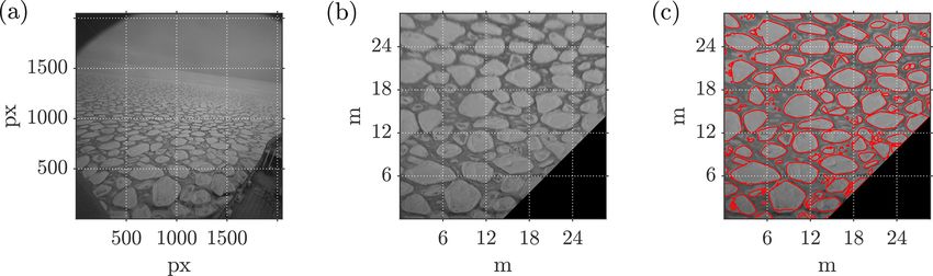
42                                    A. Alberello et al.: Pancake ice floe size distribution in the Antarctic marginal ice zone

Figure 1. Environmental conditions on 4 July 2017 (local time UTC+2). Peak wave period (a) and significant wave height (b) are sourced
from ECMWF ERA-Interim reanalysis. The magenta area denotes ice and grey dots show the ship track. In (c), which is the subdomain
indicated by a white frame in (a) and (b), ice concentration is sourced from the AMSR2 satellite with a 3.125 km resolution (Beitsch et al.,
2014). The black dots denote the position during which cameras were operational and measurements were undertaken. The green cross shows
the location of deployment of a wave buoy. In (d), pancake floe concentration reconstructed from the camera images is shown as black dots,
and total ice concentration obtained from AMSR2 satellite at the location closest to the measurements is shown as magenta squares.

in the probability density function n(D), suggesting that dif-             Shen and Ackley (1991) reported pancake floe sizes from
ferent mechanisms might in fact govern the distributions for            aerial observations collected during the Winter Weddell Sea
small and large floes (Steer et al., 2008).                             Project (July 1986), showing that pancake sizes increase with
   The power law behaviour has been verified for most cases             distance from the ice edge, from 0.1 m in the first 50 km up
but its universality has not been demonstrated yet (Horvat              to ≈ 1 m within 150 km from the edge (but without investi-
and Tziperman, 2017). Scaling parameters are typically es-              gating the floe size distribution). They attributed this to the
timated on the log–log plane with a least square fit, which             dissipation of wave energy with distance to the ice-covered
leads to biased estimates of α, and, as noted by Stern et al.           ocean and proposed a relationship between wave characteris-
(2018), without rigorous goodness-of-fit tests. In compar-              tics, mechanical ice properties and pancake size (Shen et al.,
ison, Herman et al. (2018) examined the size distribution               2004). More recently, Roach et al. (2018b) used camera im-
of floes under the action of waves in controlled laboratory             ages acquired from SWIFT buoys deployed in the Beaufort
experiments, by analysing the probability density function              Sea (Sea State cruise, October–November 2015) to quantify
n(D), which revealed a fractal response due to an arbitrary             the lateral growth of pancakes and their welding. A correla-
strain (a power law) superimposed on a Gaussian break-up                tion between wave properties and the size of relatively small
process induced by the waves. The interplay of these mecha-             pancakes (up to 0.35 m) was confirmed.
nisms is hidden in the floe number exceedance probability.                 To our knowledge, the pancake floe size distribution has
   Existing observations do not provide quantitative descrip-           yet to be characterized, noting that, although Parmiggiani
tions of the floe size distribution for pancake ice floes, which        et al. (2017) developed an algorithm for pancake floe de-
form from frazil ice under the continuous action of waves               tection, they did not provide a quantitative indication of the
and thermodynamic freezing processes (Shen et al., 2004;                shape and size of the floes. Here, a new set of images from
Roach et al., 2018b). This is important, for example, dur-              the Antarctic marginal ice zone is used to measure the shape
ing the Antarctic winter sea ice expansion, when hundreds               of individual pancakes to infer their size distribution.
of kilometres of ice cover around the Antarctic continent is
composed of pancake floes of roughly circular shape and
characteristic diameters of 0.3–3 m (Worby et al., 2008). Pan-          2   Sea ice image acquisition
cake floes represent most of the Antarctic sea ice annual mass
                                                                        At approximately 07:00 UTC on 4 July 2017, the icebreaker
budget (Wadhams et al., 2018). Moreover, in the Arctic, pan-
                                                                        S.A. Agulhas II entered the marginal ice zone between 61 and
cakes are becoming more frequent than in the past due to
                                                                        63◦ S and approximately 30◦ E during an intense storm (see
the increased wave intensity associated with the ice retreat
                                                                        Fig. 1a, b for the ship track and a snapshot of peak wave pe-
(Wadhams et al., 2018; Roach et al., 2018b).
                                                                        riod and significant wave height as sourced from ECMWF
                                                                        ERA-Interim reanalysis, Dee et al., 2011). A buoy was de-

The Cryosphere, 13, 41–48, 2019                                                                  www.the-cryosphere.net/13/41/2019/
A. Alberello et al.: Pancake ice floe size distribution in the Antarctic marginal ice zone 43
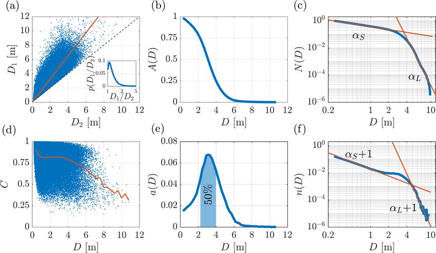
Figure 2. Sample acquired image (a), rectified and calibrated image (b) and detected pancakes (c).
ployed in the marginal ice zone ≈ 100 km from the ice edge the pancakes. Macroscopic differences between the acquired
(green mark in Fig. 1c). At the time of deployment, the sig- image and the reconstructed floes were noted; e.g. multiple
nificant wave height was 5.5 m, with maximum individual floes were detected as one (artificial welding) or individual
wave height of 12.3 m. The dominant wave period was 15 s. floes were divided by the automatic algorithm into multiple
A system of two GigE monochrome industrial CMOS floes.
cameras with a 2/3 inch sensor was installed on the monkey Identification of individual pancakes allows an estimation
bridge of the icebreaker to monitor the ocean surface. The of the individual floe areas S. An overall ice concentration
cameras were equipped with 5 mm C-mount lenses (maxi- (ic , Fig. 1d) can be computed as the ratio of the area cov-
mum aperture f/1.8) to provide a field of view of approx- ered by pancake floes to the total surface in the field of view.
imately 90◦ . The cameras were installed at an elevation of A representative concentration was estimated every 60 con-
≈ 34 m from the waterline and with their axes inclined at 20◦ secutive images (i.e. 10 min time window), which is equiv-
with respect to the horizon. The system was operated by a alent to a sampled area of 0.047 km2 . Pancake concentra-
laptop computer. Images were recorded with a resolution of tion was consistently ≈ 60 %, with no significant variations
2448 × 2048 pixels and a sampling rate of 2 Hz during day- throughout the day (Fig. 1d). The observed pancake concen-
light hours on 4 July (from 07:00 to 13:30 UTC). tration diverged from satellite observations (AMSR2) of sea
An automatic algorithm was developed using the MatLab ice concentration (see Fig. 1d), as the AMSR2 concentration
Image Processing Toolbox (Kong and Rosenfeld, 1996) to includes the interstitial frazil ice, which is intentionally ex-
extract sea ice metrics from the recorded images (see Fig. 2a cluded from the image processing (i.e. detection of pancake
for an example). To ensure statistical independence of the ice only). Moreover, satellite data are an average over two
data set (i.e. to avoid sampling the same floe twice), only one daily swaths. Due to the intense storm activity and the asso-
camera and one image was selected every 10 s for process- ciated drift of the ice edge (≈ 100 km eastward in a day) at
ing (this interval guarantees no overlap between consecutive that time, this average may not be fully representative of the
images). Images were rectified to correct for camera distor- instantaneous conditions, resulting in an under- or overesti-
tion and to project them on a common horizontal plane. A mation of the in situ ice concentration. In this regard, bridge
pixel to metre conversion was applied by imposing camera- observations following the Antarctic Sea Ice Processes and
dependent calibration coefficients. The resulting field of view Climate protocol (ASPeCt, Worby et al., 2008) indicated a
is 28 m × 28 m and the resolution of 29 px m−1 (see Fig. 2b). 90 %–100 % concentration of total ice, where pancake ice
The image was processed to eliminate the vessel from the was the primary ice type, with a concentration of 50 %–60 %
field of view, adjust the image contrast and convert the grey for most of the cruise (de Jong et al., 2018), in agreement
scales into a binary map based on a user-selected threshold. with the image processing.
The mapping isolates the solid ice shapes from background
water or frazil ice. The binary images, however, are noisy
and require refining based on morphological image process- 3 Pancake ice shape and floe size distribution
ing to improve the fidelity of the shape of identified pancake
floes (i.e. erosion, filling and expansion). Threshold selection By approximating the floe shape as an ellipse, major (D1 )
and morphological operations are optimized to detect pan- and minor (D2 ) axes are extracted. It is common practice,
cake floes only and exclude interstitial frazil ice. (The op- however, to define one representative
√ dimension as a char-
timization is performed for the specific light and ice condi- acteristic diameter D = 4S/π , by assuming that the pan-
tions using this particular camera set-up.) The resulting sepa- cake is a disk (Toyota et al., 2016), noting that other met-
rated floes are shown in Fig. 2c. Post-processed images were rics are also widely used, e.g. the mean caliper diameter
visually inspected for quality control, and ≈ 5 % of the im- (Rothrock and Thorndike, 1984). Only floes entirely within
ages were discarded due to unsatisfactory reconstruction of the field of view are considered for these operations. Detect-
ing small floes with D < 0.25 m is prone to error due to the
www.the-cryosphere.net/13/41/2019/ The Cryosphere, 13, 41–48, 201944 A. Alberello et al.: Pancake ice floe size distribution in the Antarctic marginal ice zone Figure 3. In (a) is the scatter plot of the major and minor axis of the pancake floe with the linear fit (solid orange line), the inset shows the probability density function of D1 /D2 . In (b) is the ice area distribution as a function of the floe diameter expressed as the exceedance probability. In (c) is the floe number exceedance probability N(D) as a function of the floe diameter with two power laws (solid orange lines) fitted for small (D < 2.3 m) and large floes (D > 4 m). In (d) is the scatter plot of the circularity of the floes against the equivalent diameter and the average value (solid orange line). In (e) is the ice area distribution as a function of the floe diameter expressed as probability density function. In (f) is the floe number probability density function n(D) as a function of the floe diameter with two power laws (solid orange lines) fitted for small (D < 2.3 m) and large floes (D > 4 m). limited number of pixels of which these floes are comprised Figure 3c shows the exceedance probability N (D), which and, thus, excluded from the analysis (Toyota et al., 2011). exhibits two distinct slopes in the log–log plot, with a smooth Moreover, a small fraction of large floes (< 10 % of floes transition from mild to steep slopes around the dominant larger than 5 m) were artificially welded by the image pro- diameter of 3.1 m. The probability density function of the cessing. These floes were also excluded. In total, 4×10⁵ in- equivalent diameter n(D), shown in Fig. 3f, displays a pro- dividual floes were considered over an equivalent sampled nounced hump in the transition between these regimes, re- area of ≈ 1.55 km2 and spanned almost 100 km of the non- vealing a third regime (2.3 m < D < 4 m) around the modal contiguous marginal ice zone. pancake diameter, which is hidden in the exceedance proba- Figure 3a presents a scatter plot of the aspect ratio D1 : D2 . bility, where the small- and large-floe regimes are defined as On average D1 is ≈ 60 % greater than D2 (slope of a lin- D < 2.3 m and D > 4 m (somewhat arbitrarily). ear fit). This aspect ratio is similar to the one observed for Small floes (D < 2.3 m) constitute the vast majority of the broken ice floes (Toyota et al., 2011). The inset shows the total detected floes (> 80 %). In this regime, the mild slope full probability distribution of the ratio D1 /D2 and indicates of N (D) may result from a continuous process of floe accre- that floes elongated such that D1 /D2 > 3 are infrequent. Fig- tion (from frazil to larger pancakes) regulated predominantly ure 3d shows the circularity C = 4π S/P 2 , where P is the by thermodynamic freezing processes (Roach et al., 2018b). floe perimeter (for a circle C = 1), which characterizes the Floes larger than 4 m are detected far less frequently (< 5 % shape of the floes, noting that other metrics can be used to of the total floes), and the steeper slope indicates that their define the roundness of the floes (Hwang et al., 2017). For size is most likely governed by different underlying physi- floes up to D ≈6 m, the average circularity, denoted by the cal mechanisms. Visual examination of the acquired images continuous line, is C ≥ 0.75. Similar values have been re- shows that the majority of the large floes are composed of ported for much larger broken floes (Lu et al., 2008). two or more welded pancakes, suggesting that the welding Figure 3b and 3e display the floe size area distribution as process, promoted by the high concentration of pancakes and the exceedance probability and probability density function. the presence of interstitial frazil ice (Roach et al., 2018b), Figure 3e shows that, in terms of the equivalent diameter (D), could be the dominant underlying mechanism for the shape 50 % of the pancake area is comprised of floes with diameters of the probability distribution of large floes. Finite size ef- in the range 2.3–4 m. The mode of the area distribution is fects are ruled out because the change in slope occurs for 3.1 m (median and mean are ≈ 3.1 m and ≈ 3.2 m) compared D ≈ 4 m, which is considerably smaller than the image foot- to D1 = 4 m and D2 = 2.6 m, using the major and the minor print. axes. The Cryosphere, 13, 41–48, 2019 www.the-cryosphere.net/13/41/2019/
A. Alberello et al.: Pancake ice floe size distribution in the Antarctic marginal ice zone                                      45

   Assuming, as standard, a power law N (D) ∝ D −α as a           4   Conclusions
benchmark and using the maximum likelihood method fol-
lowing Stern et al. (2018), we determine α = αS = 1.1 for         Observations of pancake ice floe sizes during the winter ex-
small floes (D < 2.3 m) and α = αL = 9.4 for large floes          pansion of the Antarctic marginal ice zone were analysed.
(D > 4 m). (Note that the maximum recorded diameter was           An automatic floe detection algorithm was used to extract
D = 10.8 m, and, therefore, the estimation of the scaling ex-     metrics (diameter and area) of√the pancake floes, for which
ponent is not particularly meaningful or robust in either of      the equivalent diameter (D = 4S/π ) ranged between 0.25
the two regimes, as less than a decade of length scales are       and 10 m. This allowed a quantitative representation of the
available.)                                                       pancake size distribution to be discussed.
   The power-law fits are approximations only, and an ob-            The floe size distribution displays three distinct regimes,
jective Kolmogorov–Smirnov goodness-of-fit test (Clauset          which are visible in the probability density function that,
et al., 2009) reveals that the empirical pancake size distribu-   compared to the commonly reported exceedance probabil-
tion does not scale accordingly to a power law in either the      ity, is more informative. One regime is D = 2.3–4 m, centred
small- or large-floe regime, noting the power law hypothesis      around the dominant pancake diameter of 3.1 m, which cov-
is more likely to be rejected when tested over limited diame-     ers half of the total pancake area, and appears as a hump in
ter ranges (i.e. less than a decade). A close inspection of the   the probability density function. Two different behaviours are
empirical distribution shows that N (D) possesses a slightly      observed for smaller and larger pancakes on a log–log plane.
concave-down curvature across all the diameter ranges (in         The small-floe regime (D < 2.3 m), in which it is conjec-
a log–log plane), which is commonly associated with a trun-       tured that pancakes are experiencing thermodynamic growth,
cated power law (Stern et al., 2018). The corresponding n(D)      is characterized by a mild negative slope (in terms of the floe
displays an S shape in the small-floe regime (it shifts from      number exceedance and probability density function), while
a concave-down to a concave-up curvature at D ≈ 1 m) in           the large-floe regime, in which floes are typically formed by
contrast to the hypothesis of a power law behaviour. Devi-        welding (detected from visual analysis), is characterized by
ations from the power law scaling are prominent towards           a much steeper slope, noting that neither of the two regimes
the extremes of the intervals (D → 0.25 m and D → 2.3 m           conform to a power law scaling.
for the small-floe regime; D → 4 m and D → 10 m for the              These results reflect observations collected under storm
large-floe regime) but become conspicuous only by examin-         conditions and, thus, lack generality. Simultaneous measure-
ing the empirical distribution over limited diameter ranges       ments of waves, floe size and heat fluxes under a number of
and probability intervals (i.e. zooming in on Fig. 3c–f). We      different conditions are needed to verify the conjecture that
also note that the increasing a(D) in the small-floe regime       different physical mechanisms (e.g. thermodynamic growth
(Fig. 3e) is inconsistent with a power law for αS ≥ 1, as the     and welding) are responsible for the peculiar shape of the
area and number distributions are proportional to each other,     pancake ice floe size distribution.
i.e. a(D) ∝ D 2 n(D). Values of αS ≥ 1 may be because the
exponent has been estimated over a range of less of decade
of diameters, making its estimation non-robust. The discrep-      Code and data availability. The detection algorithm and the ac-
ancy between area and number distribution confirms that the       quired images are available upon request to the corresponding au-
                                                                  thor.
underlying number distribution is not a power law, although
we note that αS ∈ (0.9, 1) provides a qualitatively good fit
for the number distribution and is consistent with the grow-
ing area distribution.
   Goodness-of-fit tests also rule out floe size distributions
such as the truncated power law (Stern et al., 2018), gen-
eralized Pareto (Herman, 2010) and linear combination of
Gaussian distribution and power law (Herman et al., 2018). It
appears that an accurate approximation of the floe size distri-
bution (in the goodness-of-fit sense) can only be achieved by
dropping any a priori assumptions on the functional shape,
e.g. by using a non-parametric kernel density estimation
(Botev et al., 2010). However, this does not provide any in-
sight into the underlying physical processes responsible for
the shape of the empirical distribution.

www.the-cryosphere.net/13/41/2019/                                                           The Cryosphere, 13, 41–48, 2019
46 A. Alberello et al.: Pancake ice floe size distribution in the Antarctic marginal ice zone
Appendix A: Pancake detection algorithm
The algorithm for the pancake detection is developed us-
ing the MatLab Image Processing Toolbox and built-in func-
tions.
1. Rectification: this projects the distorted camera image
on an horizontal plane based on the camera internal pa-
rameters and the angle of view.
2. Contrast adjustment: contrast in the greyscale image is
enhanced based on a CLAHE algorithm (the limit for
clipping and shape of the distribution are user selected)
to better isolate the pancakes from the frazil ice.
3. Masking: the removes the ship from the field of view.
4. Binary conversion: the greyscale image is converted
into a binary image where 1 corresponds to white (i.e.
ice) and 0 to water or frazil (the threshold for conversion
is user selected).
5. Cleaning: this morphological operation removes iso-
lated white pixels (i.e. 1s completely surrounded by 0s).
6. Erosion: this morphological operation helps to separate
the blobs corresponding to the pancakes (the erosion
value is user selected).
7. Filling: this morphological operation substitute 0 s with
1 s in area completely enclosed by white pixels.
8. Dilatation: this morphological operation counterbal-
ance the ice pixels lost by the erosion without merging
two separate blobs.
9. Clear border: this removes blobs intersecting the border
of the field of view.
10. Labelling and properties extraction: geometrical prop-
erties of each individual floe are extracted.
All thresholds are user selected and the parameters have been
subjected to testing to find the combination of operations that
provided the best reconstruction as evaluated by the user’s
visual inspection.
The Cryosphere, 13, 41–48, 2019 www.the-cryosphere.net/13/41/2019/A. Alberello et al.: Pancake ice floe size distribution in the Antarctic marginal ice zone 47
Author contributions. AA, MO and AT acquired the images. AA, Roy. Meteor. Soc., 137, 553–597, https://doi.org/10.1002/qj.828,
MO, LB and AT conceived the manuscript. AA analysed the im- 2011.
ages. MV, CE and KM provided satellite images, buoys measure- de Jong, E., Vichi, M., Mehlmann, C. B., Eayrs, C., De Kock, W.,
ments and ASPeCt observations. All authors contributed to the data Moldenhauer, M., and Audh, R. R.: Sea Ice conditions within
interpretation and to the writing of the manuscript. the Antarctic Marginal Ice Zone in WInter 2017, onboard the SA
Agulhas II, https://doi.org/10.1594/PANGAEA.885211, 2018.
Gherardi, M. and Lagomarsino, M. C.: Characterizing the
Competing interests. The authors declare that they have no conflict size and shape of sea ice floes, Sci. Rep., 5, 10226,
of interest. https://doi.org/10.1038/srep10226, 2015.
Herman, A.: Sea-ice floe-size distribution in the context of sponta-
neous scaling emergence in stochastic systems, Phys. Rev. E, 81,
Acknowledgements. The cruise was funded by the South African 066123, https://doi.org/10.1103/PhysRevE.81.066123, 2010.
National Antarctic Programme through the National Research Herman, A., Evers, K.-U., and Reimer, N.: Floe-size distributions in
Foundation. This work was motivated by the Antarctic Circum- laboratory ice broken by waves, The Cryosphere, 12, 685–699,
navigation Expedition (ACE) and partially funded by the ACE https://doi.org/10.5194/tc-12-685-2018, 2018.
Foundation and Ferring Pharmaceuticals. Support from the Aus- Horvat, C. and Tziperman, E.: A prognostic model of the sea-ice
tralian Antarctic Science Program (project 4434) is acknowledged. floe size and thickness distribution, The Cryosphere, 9, 2119–
Miguel Onorato was supported by the “Departments of Excellence 2134, https://doi.org/10.5194/tc-9-2119-2015, 2015.
2018–2022” grant awarded by the Italian Ministry of Education, Horvat, C. and Tziperman, E.: The evolution of scaling laws in
University and Research (MIUR) (L.232/2016). Clare Eayrs was the sea ice floe size distribution, J. Geophys. Res.-Oceans, 122,
supported under NYUAD Center for the Global Sea Level Change 7630–7650, https://doi.org/10.1002/2016JC012573, 2017.
project G1204. The authors thank Lotfi Aouf at Meteo France for Hwang, B., Wilkinson, J., Maksym, E., Graber, H. C., Schweiger,
providing reanalysis data and the editor, Ted Maksym, for useful A., Horvat, C., Perovich, D. K., Arntsen, A. E., Stanton, T. P.,
comments. Alberto Alberello and Alessandro Toffoli acknowl- Ren, J., and Wadhams, P.: Winter-to-summer transition of Arctic
edge support from the Air-Sea-Ice Lab Project. Miguel Onorato sea ice breakup and floe size distribution in the Beaufort Sea,
acknowledges Barbara GiuliNico for interesting discussions. Elem. Sci. Anth., 5, p. 40, https://doi.org/10.1525/elementa.232,
Alberto Alberello, Alessandro Toffoli and Miguel Onorato thank 2017.
Le Fascette for technical support during the cruise. Kong, T. Y. and Rosenfeld, A.: Topological algorithms for digital
image processing, vol. 19, Elsevier, 1996.
Edited by: Ted Maksym Lu, P., Li, Z. J., Zhang, Z. H., and Dong, X. L.: Aerial obser-
Reviewed by: Christopher Horvat and one anonymous referee vations of floe size distribution in the marginal ice zone of
summer Prydz Bay, J. Geophys. Res.-Oceans, 113, C02011,
https://doi.org/10.1029/2006JC003965, 2008.
Parmiggiani, F., Moctezuma-Flores, M., and Guerrieri, L.: Identify-
ing pancake ice and computing pancake size distribution in aerial
References photographs, in: Remote Sensing of the Ocean, Sea Ice, Coastal
Waters, and Large Water Regions 2017, vol. 10422, International
Beitsch, A., Kaleschke, L., and Kern, S.: Investigating high- Society for Optics and Photonics, 2017.
resolution AMSR2 sea ice concentrations during the February Roach, L., Horvat, C., Dean, S., and Bitz, C.: An emergent
2013 fracture event in the Beaufort Sea, Remote Sens., 6, 3841– Sea Ice Floe Size Distribution in a Global Coupled Ocean–
3856, https://doi.org/10.3390/rs6053841, 2014. Sea Ice Model, J. Geophys. Res.-Oceans, 123, 4322–4337,
Bennetts, L. G., O’Farrell, S., and Uotila, P.: Brief commu- https://doi.org/10.1029/2017JC013692, 2018a.
nication: Impacts of ocean-wave-induced breakup of Antarc- Roach, L., Smith, M., and Dean, S.: Quantifying Growth
tic sea ice via thermodynamics in a stand-alone version of of Pancake Sea Ice Floes Using Images From Drift-
the CICE sea-ice model, The Cryosphere, 11, 1035–1040, ing Buoys, J. Geophys. Res.-Oceans, 123, 2851–2866,
https://doi.org/10.5194/tc-11-1035-2017, 2017. https://doi.org/10.1002/2017JC013693, 2018b.
Botev, Z. I., Grotowski, J. F., and Kroese, D. P.: Kernel density es- Rothrock, D. A. and Thorndike, A. S.: Measuring the sea ice
timation via diffusion, Ann. Stat., 38, 2916–2957, 2010. floe size distribution, J. Geophys. Res.-Oceans, 89, 6477–6486,
Clauset, A., Shalizi, C., and Newman, M.: Power-Law Dis- https://doi.org/10.1029/JC089iC04p06477, 1984.
tributions in Empirical Data, SIAM Rev., 51, 661–703, Shen, H. H. and Ackley, S. F.: A one-dimensional model for
https://doi.org/10.1137/070710111, 2009. wave-induced ice-floe collisions, Ann. Glaciol., 15, 87–95,
Dee, D., Uppala, S., Simmons, A., Berrisford, P., Poli, P., https://doi.org/10.3189/1991AoG15-1-87-95, 1991.
Kobayashi, S., Andrae, U., Balmaseda, M., Balsamo, G., Bauer, Shen, H. H., Ackley, S. F., and Yuan, Y.: Limiting diame-
P., Bechtold, P., Beljaars, A., van de Berg, L., Bidlot, J., Bor- ter of pancake ice, J. Geophys. Res.-Oceans, 109, C12035,
mann, N., Delsol, C., Dragani, R., Fuentes, M., Geer, A., Haim- https://doi.org/10.1029/2003JC002123, 2004.
berger, L., Healy, S., Hersbach, H., Hólm, E., Isaksen, L., Kåll- Steele, M.: Sea ice melting and floe geometry in a simple
berg, P., Köhler, M., Matricardi, M., McNally, A., Monge-Sanz, ice-ocean model, J. Geophys. Res.-Oceans, 97, 17729–17738,
B., Morcrette, J., Park, B., Peubey, C., de Rosnay, P. C. T., Thé- https://doi.org/10.1029/92JC01755, 1992.
paut, J., and Vitart, F.: The ERA–Interim reanalysis: configu-
ration and performance of the data assimilation system, Q. J.
www.the-cryosphere.net/13/41/2019/ The Cryosphere, 13, 41–48, 201948 A. Alberello et al.: Pancake ice floe size distribution in the Antarctic marginal ice zone Steer, A., Worby, A., and Heil, P.: Observed changes in Worby, A. P., Geiger, C. A., Paget, M. J., Van Woert, M. L., sea-ice floe size distribution during early summer in the Ackley, S. F., and DeLiberty, T. L.: Thickness distribution western Weddell Sea, Deep-Sea Res. Pt. II, 55, 933–942, of Antarctic sea ice, J. Geophys. Res.-Oceans, 113, C05S92, https://doi.org/10.1016/j.dsr2.2007.12.016, 2008. https://doi.org/10.1029/2007JC004254, 2008. Stern, H., Schweiger, A., Zhang, J., and Steele, M.: On reconciling Zhang, J., Schweiger, A., Steele, M., and Stern, H.: Sea ice floe disparate studies of the sea-ice floe size distribution, Elem. Sci. size distribution in the marginal ice zone: Theory and numer- Anth., 6, p. 49, https://doi.org/10.1525/elementa.304, 2018. ical experiments, J. Geophys. Res.-Oceans, 120, 3484–3498, Toyota, T., Haas, C., and Tamura, T.: Size distribution and shape https://doi.org/10.1002/2015JC010770, 2015. properties of relatively small sea-ice floes in the Antarctic Zhang, J., Stern, H., Hwang, B., Schweiger, A., Steele, M., Stark, marginal ice zone in late winter, Deep-Sea Res. Pt. II, 58, 1182– M., and Graber, H. C.: Modeling the seasonal evolution of 1193, https://doi.org/10.1016/j.dsr2.2010.10.034, 2011. the Arctic sea ice floe size distribution, Elem. Sci. Anth., Toyota, T., Kohout, A., and Fraser, A. D.: Formation processes of 4, p. 000126, https://doi.org/10.12952/journal.elementa.000126, sea ice floe size distribution in the interior pack and its relation- 2016. ship to the marginal ice zone off East Antarctica, Deep-Sea Res. Pt. II, 131, 28–40, https://doi.org/10.1016/j.dsr2.2015.10.003, 2016. Wadhams, P., Aulicino, G., Parmiggiani, F., Persson, P. O. G., and Holt, B.: Pancake Ice Thickness Mapping in the Beaufort Sea From Wave Dispersion Observed in SAR Imagery, J. Geophys. Res.-Oceans, 123, 2213–2237, https://doi.org/10.1002/2017JC013003, 2018. The Cryosphere, 13, 41–48, 2019 www.the-cryosphere.net/13/41/2019/
You can also read