Deep learning for prediction of complex geology ahead of drilling
←
→
Page content transcription
If your browser does not render page correctly, please read the page content below
Deep learning for prediction of complex geology
                                                         ahead of drilling

                                                Kristian Fossum1 , Sergey Alyaev1 , Jan Tveranger1 , Ahmed Elsheikh2
                                                          1
                                                            NORCE Norwegian Research Centre, Bergen, Norway
                                           2
                                               School of Energy, Geoscience, Infrastructure and Society, Heriot-Watt University,
arXiv:2104.02550v1 [stat.ML] 6 Apr 2021

                                                                        Edinburgh, United Kingdom

                                                  Abstract. During a geosteering operation the well path is intentionally
                                                  adjusted in response to the new data acquired while drilling. To achieve
                                                  consistent high-quality decisions, especially when drilling in complex en-
                                                  vironments, decision support systems can help cope with high volumes
                                                  of data and interpretation complexities. They can assimilate the real-
                                                  time measurements into a probabilistic earth model and use the updated
                                                  model for decision recommendations.
                                                  Recently, machine learning (ML) techniques have enabled a wide range
                                                  of methods that redistribute computational cost from on-line to off-
                                                  line calculations. In this paper, we introduce two ML techniques into
                                                  the geosteering decision support framework. Firstly, a complex earth
                                                  model representation is generated using a Generative Adversarial Net-
                                                  work (GAN). Secondly, a commercial extra-deep electromagnetic simu-
                                                  lator is represented using a Forward Deep Neural Network (FDNN).
                                                  The numerical experiments demonstrate that the combination of the
                                                  GAN and the FDNN in an ensemble randomized maximum likelihood
                                                  data assimilation scheme provides real-time estimates of complex geo-
                                                  logical uncertainty. This yields reduction of geological uncertainty ahead
                                                  of the drill-bit from the measurements gathered behind and around the
                                                  well bore.

                                                  Keywords: Geosteering · Machine Learning · Deep Neural Network ·
                                                  Generative Adversarial Network · Ensemble randomized maximum like-
                                                  lihood

                                          1     Introduction
                                          The process of drilling wells for hydrocarbon production represents a major cost
                                          in petroleum reservoir development. However, drilling of new wells is necessary
                                          to increase the total oil recovery. To maximize the value for each drilled well it
                                          is necessary to optimize the placement of the well within the reservoir structure.
                                          An optimally placed well will mobilize more of the petroleum resources, and
                                          reduce the need for injected water – reducing the environmental impact of oil
                                          production.
                                              To place a well in its optimal position, operators apply geosteering. Here, the
                                          well trajectory is adjusted while drilling in response to real-time measurement
2 K. Fossum et al.
of the geology surrounding the drill bit. The value of geosteering has been well
documented in the literature [1,17,19].
The main objective with geosteering is to utilize the information in the mea-
surements to make optimal decisions. Hence, geosteering can be seen as a se-
quential decision process under uncertainty and should be treated in a prob-
abilistic framework [20]. Recently, a workflow based on the Ensemble Kalman
Filter (EnKF) [12] has been employed to condition the geological model on
measurements acquired while drilling [9,22]. In the EnKF the uncertainty is rep-
resented by an ensemble of equiprobable realizations. This workflow has then
been combined with a global optimization method and applied as a Decision
Support System (DSS)[3].
The DSS framework provides high quality decisions on synthetic cases, but
practical challenges should be addressed for it to be applicable to real opera-
tions [3]. Firstly, to our knowledge, there is no studies which combine the en-
semble update with a commercial tool for simulation of measurements. Secondly,
the earth model utilized in the published studies does not represent a realistic
geological complexity. Conceptually, it is easy to insert any numerical model for
simulating the measurements into the DSS workflow. Similarly, there is nothing
that prohibits the use of complex earth models. However, as the complexity in-
crease, the numerical run-time also increases hindering real-time performance.
Moreover, complex earth models can not typically be represented using a Gaus-
sian distribution, and consequently EnKF updates will not retain the geological
complexity [28].
Extra-Deep EM logs Decision
Actual
measurements
Ensemble of Global well-
Updated earth models: Current realizations
EnRML GAN placement
realizations Predictions ahead of bit
parametrization optimization
Predicted Bayesian
measurements update
Structures
1D local
FDNN EM model and facies generation
model
From GAN
Fig. 1: The proposed DSS workflow. Green boxes highlight the new elements
introduced in this paper.
In this paper, we introduce important elements to make the DSS better suited
to real operations, see Figure 1. The main novelty in our approach is to introduce
a machine-learning method to represent both the earth model and the forward
model of extra-deep borehole electromagnetic (EM) measurements. Within thisDeep learning for prediction of complex geology ahead of drilling 3
setting we demonstrate that a real-time ensemble-based inversion can indeed
predict the distribution of non-trivial geology ahead of bit.
To construct a reference earth model we generate realizations of a fluvial
geological environment using a commercial software. These realizations are then
sub-sampled to form a training dataset for the offline training of a Generative
Adversarial Network (GAN). The GAN is then used, online, to generate plau-
sible geological realizations from a low-dimensional Gaussian input vector. The
earth modeling is described in Section 2. For modeling the extra-deep EM mea-
surements we use a forward deep neural network (FDNN) trained on a dataset
generated using a commercial simulator (Section 3). In Section 4 we discuss the
exact and the fast data assimilation (DA) methods. The numerical results, show-
ing the applicability of our proposed method are given in Section 5. Finally, we
summarize and conclude the paper in Section 6.
2 Earth modeling using GAN
GANs are a class of unsupervised machine learning methods which can learn to
generate new formatted data with the same statistics as the training set. Mo-
tivated by successful applications of GANs for modeling channelized structures
for reservoir simulation [8,7], we use a GAN for efficient earth modeling.
The GAN consists of two deep neural networks (DNNs): a generator and a
discriminator. The generator takes a random Gaussian low dimensional vector as
input and generates a realization of formatted data: geological realization. The
discriminator takes the formatted data and gives a probability of it being ’real’,
i.e., belonging to the training set. During training the DNNs contest each other
in a min-max game. They are trained simultaneously. On each training step the
generator creates (fake) geological realization from random vectors. Fake geo-
logical realizations are combined with random samples of real earth model and
are fed to the discriminator. The loss function for the generator is proportional
to number of ’fakes’ correctly identified by the discriminator. The loss function
for the discriminator is proportional to the total misjudged data samples. In
our study we use an adapted Wasserstein GAN with hierarchical convolutional
networks for the generator and the discriminator, see [4] for implementation
details.
For geosteering we want to reproduce likely geological realizations of facies
and porosity distributions on a 2D vertical geological section along the well to
identify the oil-bearing sands ahead of bit. For training of GAN we use a large
(compare to the area of prediction) reference earth model, which should provide
a realistic test case for the present study in terms of scale and actual geological
features and properties. The reference earth model is constructed using a com-
mercial software that models a synthetic structural framework, a facies model
set-up derived from outcrop analogue data, and synthetic petrophysical proper-
ties of individual facies derived from published literature. The resulting model
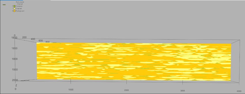
measures 4000m x 1000m x 200m (xyz) with cell dimensions set to 10x10x0.5 m,
yielding a regular corner-point grid of size 400x100x400, see Figure 2.4 K. Fossum et al.
Fig. 2: The original earth model generated by the commercial tool.
The constructed facied model represents a low net/gross fluvial depositional
system. It was chosen since it provides complex 3D architectures comprising
a limited number of facies, which form contrasting geometries, see Figure 2.
Input numbers for statistical generation of facies and geometries are derived from
a well-documented outcrop of the Cretaceous lower Williams Fork Formation
(Mesa Verde Group) at Coal Canyon, Colorado, USA [26,27,30].
Key parameters of the facies model set-up are listed in Table 1. The model is
not intended as a rendering of the outcrop itself and is consequently simplified
compared to descriptions of the original outcrop [11,24,25,27]. The model con-
tains three facies: Background/shale, Channels and Crevasse splays. The prob-
ability distribution of channel width in the model is adapted to include “nar-
row channel bodies”, and stacking of channels accounts for multi-story channels
which comprise more than 80% of the observed channel bodies. The flow direc-
tion of the channel system is set towards 45 ± 10 degrees. No trends were used
to condition the spatial distribution of channels.
Table 1: Parameter settings for facies models.
Volumetric fraction Value Tolerance Comments
Channel system volume fraction 0.3 0.05
Channel positioning 1 No trends
Crevasse volume fraction 0.1 0.03 Of channel system vol. frac.
Channel geometry Value SD Min. Max.
Thickness 4.2 1.5 Form/repulsion Setting
Width 155 50 20 500
Cross-section geometry Parabolic, basic variability
Correlation W/T 36
Channel form Rigid
Amplitude 400 50
Repulsion None
Sinuosity 1.3
Azimuth 45 10Deep learning for prediction of complex geology ahead of drilling 5
The geological realization is parameterized by a vector of 60 independent
parameters. For each 60-dimensional vector, the generator outputs a 64x64
grid with three values in each grid block. For a grid block (with dimensions
10.0m along-well and 0.5m thickness) the three values, ’channels’, represent
the probability of the grid-block belonging to the respective facies class: Back-
ground/Channel/Crevasse. Our generator is also predicting porosity/resistivity
distribution within the geo-bodies, but in this initial study only the facies classes
are used.
For training, the original 3D earth model is sampled as 64x64 2D images with
three channels. The facies index from the training set is converted into one-hot
three-dimensional vector. That is, the vector represents the probability of facies:
the value of the true index is set to one and other channels to zero. During
evaluation, the resistivity of the facies with highest probability is applied.
3 LWD Neural Network
To maintain real-time performance of a data assimilation workflow the forward
model should be fast and support batch, preferably parallel execution. Propri-
etary forward models provided by measurement instrument vendors provide the
most accurate results, but they are often not sufficiently fast, and not always op-
timized for batch execution. In [2], the authors developed a DNN approximation
of such a forward model [29], which we abbreviate FDNN.
The model approximates the output of the ultra-deep electromagnetic well-
bore logging instrument. The instrument is configured to transmit four shallow
and nine pairs of deep directional measurements, and has sensitivity to bound-
aries up to 30 meters to the side from the well bore. We emphasize that the
tool provides information around, but not ahead of the drilling position. An
illustration of the deep measurements is provided in Figure 3.
The input to the FDNN model is a layered geological media with up to
three boundaries above and below the measurement instrument as well as the
resistivity values of all seven layers. In this study we assume that the layer
resistivity is isotropic and that the well is aligned with the horizontal axis.
We produce one synthetic set of measurements for every horizontal position
of the gridded model which we ’drill’ through. First, we choose most probable
facies for each ’pixel’ and substitute it with the corresponding resistivity value:
1. Background, R = 220.0 Ohm m;
2. Channel, R = 3.6 Ohm m;
3. Crevasse, R = 4.1 Ohm m.
Second, we find boundaries between layers composed of pixels with equal resis-
tivities and use them as the input to the forward model.
4 Data assimilation
In the DSS for geosteering [3], one uses data assimilation to condition the earth
model to measurements made while drilling. The fundamental idea is that if a6 K. Fossum et al.
32 m.
0 m.
640 m.
Fig. 3: Resistivity of earth model plotted in 1:2 aspect ratio. The green lines
shows the measurements and their extent illustrate the maximum sensitivity
depth. The full red line is the drilled well, and the dashed red lines indicate the
potential for geosteering.
poorly known earth model can be made consistent with measurements it will
provide more accurate forecasts, and, hence, provide a better basis for decisions.
In this paper, the emphasis is placed on the data assimilation part of the
DSS. Especially data assimilation utilizing an efficient neural network model
for the synthetic logs, and an efficient GAN-generator for representing complex
earth models. To check whether this setup provides useful conditioned models
we consider two data assimilation algorithms. Firstly, the Markov Chain Monte
Carlo (MCMC), which is considered as a gold standard method for sampling.
Secondly, the ensemble randomized maximum likelihood (EnRML), an approx-
imate method suitable for DSS.
4.1 MCMC
A reliable method for sampling from a complex posterior distribution is the
MCMC technique. MCMC relates to the general framework of methods intro-
duced in [23] and [18] for Monte Carlo (MC) integration. One designs a Markov
chain that produce samples from the desired posterior distribution, and subse-
quently utilize these samples for MC estimation. In this section, the adaptive
Metropolis-Hastings method, utilized in the numerical study, is introduced. For
more information on MCMC we refer the reader to [6], and references therein.
Suppose we want samples from the un-normalized posterior distribution F ,
which is the general case with the Bayesian method where the normalizing factor
often is very difficult to calculate. Assume that the current element is m,~ and that
the chain proposes a move to m ~ ∗ , with conditional probability density q (m
~ ∗ |m).
~
The move is performed with probability
b (m,
~ m~ ∗ ) = min (1, r (m,
~ m~ ∗ )) (1)
where the Hastings ratio is defined as
~ ∗ ) q (m|
F (m ~ m ~ ∗)
r (m,
~ m~ ∗) = . (2)
F (m)
~ q (m ~ ∗ |m)
~
If the move is not made m ~ ∗ = m.
~ This is the basis for the Metropolis-Hastings
method, and it can be shown that the method will generate samples from the
posterior distribution F .Deep learning for prediction of complex geology ahead of drilling 7
The Metropolis-Hastings algorithm requires a choice of proposal distribution,
and some distributions will work better than others. Intuitively, one would like
to draw proposal samples from F . However, this is not possible since we cannot
sample from this distribution. However, one idea is to consider the previous
samples from the algorithm as approximate samples from F . With this approach
proposal samples are drawn from
2.382
∗
m~ ∼ (1 − β) N m, ~ C̃m
~ + βN (m,~ Qm ~ ), (3)
Nm
where C̃m ~ is the empirical covariance matrix calculated utilizing all the preced-
ing iterations of the Markov Chain, Qm ~ is some fixed non-singular matrix and
0 < β < 1. Note that β = 1 until Cm ~ is well defined. This sampling method was
applied in [13,14]. It is well known that the MCMC requires a certain burn-in
period, since the initial samples are not from the posterior distribution. Hence,
it is necessary to monitor the convergence of the method. In this work, conver-
gence is monitored by assessing the maximum root statistic of the multivariate
potential scale reduction factor [5].
4.2 EnRML
The EnRML [16] has recently become one of the most successful methods for au-
tomatic history matching of petroleum reservoirs. The EnRML is based on min-
imization of an objective function using the ensemble approximation of the sen-
sitivity matrix. Hence, the EnRML can be formulated in many different ways. In
this study we utilize the approximate form of the Levenberg-Marquardt method,
introduced in [10].
Iteration number i of the Levenberg-Marquardt method is given as
h i−1
−1 T −1
δm~ i = − (1 + λi ) Cm
~ + Gi Cd~ Gi (4)
h i
× Cm −1
~ (m~i−m ~ prior ) + GTi C −1
~ ~ − d~obs + ~
g (m) (5)
d
where λi is the Levenberg-Marquardt
multiplier, G is the sensitivity of data to
the parameters, and ~ ∼ N 0, Cd~ is a realization of the measurement observa-
tion noise.
In the ensemble framework, we approximate Cm ~ and G using the ensemble.
To this end we define
1/2 ~ −1
G̃ = Csc ∆d (∆m)~ (6)
C̃m
~ = ∆m∆
~ m~T (7)
where
√
1
∆m
~ = [m ~ 1, . . . , m ~ N ] IN − 11T / N − 1,
~ j, . . . , m (8)
N
√
1
∆d~ = Csc
−1/2
[g (m
~ 1 ) , . . . , g (m ~ N )] IN − 11T / N − 1,
~ j ) , . . . , g (m (9)
N8 K. Fossum et al.
N denotes the ensemble size, and Csc is a diagonal matrix for scaling the data,
typically containing the measurement variance on the diagonal. We get the ap-
proximate version of the Levenberg-Marquardt update equation by inserting en-
semble approximations of G and Cm ~ , neglecting the updates from the model
−1 −1
mismatch term, substituting the prior precision matrix Cm with C̃m
~ i , and
rewriting the equation using the Sherman-Woodbury-Morrison matrix inversion
formula [15]
h i−1
~ i = −C̃m
δm T
~ i G̃i (1 + λi ) Cd~ + G̃i C̃m
T
~ i G̃i ~ − d~obs + ~ .
g (m) (10)
The update equation is simplified by calculating the truncated singular value
decomposition of ∆d
∆d~ = Up Sp VpT , (11)
where the subscript p indicates the number of singular values that are kept. In
this work, we define p such that the cumulative sum of the p singular values
equals 99% of the cumulative sum of all the singular values. Further, to allow
for correlated measurement errors, we substitute CD with the ensemble approx-
imation C̃D
C̃d~ = ∆~∆~T , (12)
where
√
1
∆~ = [~1 , . . . ,~j , . . . ,~N ] IN − 11T / N − 1. (13)
N
Inserted into (10) gives
h i
−1/2 −1/2
~ i = −∆m
δm ~ i Vp (1 + λi ) Sp−1 UpT Cscl ∆~∆~T Cscl Up SP−T + I
T −1/2
Up Sp−1 Csc ~ − d~obs + ~
g (m) (14)
T −1/2
−1
= −∆m ~ i Vp Z [(1 + λi ) ζ + I] Up Sp−1 Z Csc ~ − d~obs + ~ ,
g (m)
−1/2 −1/2
where Z and ζ are the eigenvectors and eigenvalues of Sp−1 UpT Cscl ∆~∆~T Cscl Up SP−T .
The iterative scheme is run until it is converged. Here, we consider the method
to be converged when the relative difference in the data misfit is below a given
threshold.
5 Numerical Results
We, throughout, utilize the generative neural network, introduced in section 2,
to represent the poorly known earth model. Hence, realizations of the earth
model is generated by applying the generative network to parameters sampled
from the multivariate standard distribution, m ~ ∼ N (0, Cm ~ ). The numerical
investigation considers a well drilled horizontally, approximately, in the center
of the model and through the 9 first grid-cells. For each drilled grid-cell we
simulate measurements using the model introduced in section 3.Deep learning for prediction of complex geology ahead of drilling 9
Throughout the investigation, we consider a diagonal Cm
~ with elements equal
to 1 × 10⁻⁶ . Figure 4 shows two random earth model realizations from the prior
model. From the figure, we observe that this setup provides significant variation
in the earth model.
(a) (b) (c) (d)
(e) (f) (g) (h)
(i) (j) (k) (l)
Fig. 4: Rows 1-3 show three realizations from the prior ensemble. Each row shows
the three output channels (e.g. fig. a-c) of GAN corresponding to probability of
facies (Background/Channel/Crevasse), and the derived resistivity image (e.g.
fig. d). Red stars indicate measurement position.
The synthetic true earth model is also drawn from the prior model. All 3
channels and the derived resistivity of the synthetic truth is illustrated in figure 5.
The true observations are simulated using the true earth model.
For each of the 9 measurements positions the measurement standard devia-
tion is given as 5% of the measurement value. In addition, we let the measure-
ments at each position be correlated. Assuming equidistance between measure-
ments, the correlation length equals 10 times the inter-measurement distance.
We further assume that the measurements at two different well positions are
uncorrelated.
We conduct two numerical experiments. Firstly, we conduct a MCMC run to
properly characterize the posterior distribution. Here, 8 chains are run in parallel
for 106 iteration. At that point the chains were converged, and we extract samples10 K. Fossum et al.
(a) (b) (c) (d)
Fig. 5: (a)-(c): Facies probabilities from GAN for the synthetic truth. (d): Derived
resistivity for the synthetic truth. Red stars indicate measurement positions.
from the posterior by, for each of the 8 chains, removing the first half of the
chain and retaining every 100 iteration from the second half of the chain. Hence,
leaving 4 × 10⁴ samples from the posterior distribution. Secondly, we estimate
the posterior distribution using the EnRML method introduced in section 4.2.
Due to the fast simulation time we utilized an ensemble size of N = 500, and
in addition we applied the correlation based localization technique introduced
in [21]. The method is allowed to iterate until the relative improvement of the
updates is less than 1%. When showing the numerical results we will only plot
the values of the derived resistivity.
5.1 MCMC
Based on the posterior realizations obtained by the MCMC, we calculate the
posterior mean and posterior standard deviation, shown in figure 6 (a) and (b).
In figure 6 (c) and (d) we plot two random realizations from the posterior.
(a) (b) (c) (d)
Fig. 6: (a): MCMC mean of the resistivity. (b): MCMC standard deviation of the
resistivity. (c): Resistivity for MCMC posterior realization 1. (d): Resistivity for
MCMC posterior realization 2. Red stars indicate measurement positions.
The MCMC result illustrates that the generative neural network can be uti-
lized for data assimilation, and be successfully conditioned to measurements
utilizing a neural network proxy model. The model standard deviation is sig-
nificantly reduced close to the drill bit, and also ahead of the drill bit position.Deep learning for prediction of complex geology ahead of drilling 11
Moreover, the mean value shows that the correct resitivity is identified in these
areas. Note that the posterior still has significant variance in most parts of the
field. The areas directly around the drill bit have not obtained sufficient reduc-
tion of the standard deviation. We do not properly understand why this is so,
however, it indicates that there measurements are less sensitive to the region
near the drill bit.
5.2 EnRML
After the EnRML has converged we calculate the mean and standard deviation
from the ensemble. These are approximations to the true posterior mean and
standard deviations, and are shown in figure 7 (a) and (b). In addition, the
results from two random realizations are illustrated in figure 7 (c) and (d).
(a) (b) (c) (d)
Fig. 7: (a): Mean resistivity from the EnRML. (b): Standard deviation of the
resistivity from the EnRML. (c): Resistivity for EnRML realization 1. (d): Re-
sitivity for EnRML realization 2. Red stars indicate measurement positions.
The results for the EnRML show a significant reduction in the standard devi-
ation around the drill bit, and from the mean model we observe that the correct
facies is identified for these regions. There is some reduction of the standard
deviation ahead of the drill bit, but we observe that the variance is retained in
most of the field.
6 Summary and conclusions
In this paper, we have demonstrated that two essential parts, the earth model
and the simulated log, of an ensemble based DSS system can be substituted with
neural networks. For the earth model we utilize the GAN trained with images
from a realistic geological setting, for the simulated log we use a deep neural
network trained using a large set of simulations from a commercial tool. The
setup redistributes the computational cost from on-line to off-line calculations,
enabling complex earth models utilizing simulated logs with high accuracy to be
used in the real time DSS. The numerical results illustrate that DSS, equipped
with the GAN, provides good predictions ahead of drilling when conditioning to
only measurements with sideways sensitivity.12 K. Fossum et al.
The proposed approach has many beneficial factors. Firstly, a GAN provides
large flexibility for defining the geological setting. Here, we consider three dif-
ferent facies, but one can easily imagine the inclusion of features like faults and
pinch-outs as well as smoothly-varying properties. Secondly, we only need to
condition a few parameters with Gaussian distribution to the measurements,
which is very beneficial for the ensemble based DA approach. Thirdly, since we
are utilizing a neural network model to generate the simulated log the compu-
tational cost of simulating a single ensemble member is very low. Hence, the
proposed approach can utilize a large ensemble for the DA part.
The numerical experiments illustrated that the setup provides a reasonable
posterior distribution, and we can estimate this using the EnRML approxima-
tion. In this study we have only considered a single part of the DSS, namely the
conditioning of the earth model to measured data. However, due to the promising
results, the developments shown in this paper will integrate with the framework
developed in [3]. Hence, allowing DSS under much more complex geological set-
ting. Demonstrating the complete DSS with the proposed setup is left for future
work.
Acknowledgments
The authors are supported by the research project ’Geosteering for IOR’ (NFR-
Petromaks2 project no. 268122) which is funded by the Research Council of
Norway, Aker BP, Equinor, Vår Energi and Baker Hughes Norway.
References
1. Al-Fawwaz, A., Al-Yosef, O., Al-Qudaihy, D., Al-Shobaili, Y., Al-Faraj, H., Maeso,
C., Roberts, I.: Increased Net to Gross Ratio as the Result of an Advanced
Well Placement Process Utilizing Real-Time Density Images. In: IADC/SPE
Asia Pacific Drilling Technology Conference and Exhibition. pp. 151–160. Soci-
ety of Petroleum Engineers (apr 2004). https://doi.org/10.2118/87979-MS, http:
//www.onepetro.org/doi/10.2118/87979-MS
2. Alyaev, S., Shahriari, M., Pardo, D., Omella, A.J., Larsen, D., Jahani, N., Suter,
E.: Modeling extra-deep em logs using a deep neural network. arXiv preprint
arXiv:2005.08919, accepted in SEG Geophysics (2020)
3. Alyaev, S., Suter, E., Bratvold, R.B., Hong, A., Luo, X., Fossum,
K.: A decision support system for multi-target geosteering. Journal of
Petroleum Science and Engineering 183(August), 106381 (dec 2019).
https://doi.org/10.1016/j.petrol.2019.106381, https://doi.org/10.1016/j.petrol.
2019.106381https://linkinghub.elsevier.com/retrieve/pii/S0920410519308022
4. Arjovsky, M., Chintala, S., Bottou, L.: Wasserstein GAN. arXiv (jan 2017), http:
//arxiv.org/abs/1701.07875
5. Brooks, S.P., Gelman, A.: General Methods for Monitoring Convergence
of Iterative Simulations. J. Comput. Graph. Stat. 7(4), 434 (dec 1998).
https://doi.org/10.2307/1390675, http://www.tandfonline.com/doi/abs/10.1080/
10618600.1998.10474787http://www.jstor.org/stable/1390675?origin=crossrefDeep learning for prediction of complex geology ahead of drilling 13
6. Brooks, S.P., Gelman, A., Jones, G.L., Meng, X.L. (eds.): Handbook of Markov
Chain Monte Carlo. Chapman and Hall / CRC (2011)
7. Chan, S., Elsheikh, A.H.: Parametric generation of conditional geological realiza-
tions using generative neural networks. Computational Geosciences 23(5), 925–952
(oct 2019). https://doi.org/10.1007/s10596-019-09850-7, http://link.springer.com/
10.1007/s10596-019-09850-7
8. Chan, S., Elsheikh, A.H.: Parametrization of Stochastic Inputs Using Gener-
ative Adversarial Networks With Application in Geology. Frontiers in Water
2(March), 1–21 (mar 2020). https://doi.org/10.3389/frwa.2020.00005, https://
www.frontiersin.org/article/10.3389/frwa.2020.00005/full
9. Chen, Y., Lorentzen, R.J., Vefring, E.H.: Optimization of Well Trajectory Under
Uncertainty for Proactive Geosteering. SPE Journal 20(02), 368–383 (apr 2015).
https://doi.org/10.2118/172497-PA, https://onepetro.org/SJ/article/20/02/368/
206467/Optimization-of-Well-Trajectory-Under-Uncertainty
10. Chen, Y., Oliver, D.S.: Levenberg–Marquardt forms of the iterative ensemble
smoother for efficient history matching and uncertainty quantification. Com-
put. Geosci. (may 2013). https://doi.org/10.1007/s10596-013-9351-5, http://link.
springer.com/10.1007/s10596-013-9351-5
11. Cole, R.D., Cumella, S.: Sand-body architecture in the lower Williams Fork Forma-
tion (Upper Cretaceous), Coal Canyon, Colorado, with comparison to the Piceance
Basin subsurface. Mountain Geologist 42, 85–107 (2005)
12. Evensen, G.: Sequential data assimilation with a nonlinear quasi-geostrophic model
using Monte Carlo methods to forecast error statistics. J. Geophys. Res. 99(C5),
10143 (1994). https://doi.org/10.1029/94JC00572, http://doi.wiley.com/10.1029/
94JC00572
13. Fossum, K., Mannseth, T.: Parameter sampling capabilities of sequential and
simultaneous data assimilation: II. Statistical analysis of numerical results.
Inverse Problems 30(11), 114003 (nov 2014). https://doi.org/10.1088/0266-
5611/30/11/114003, http://stacks.iop.org/0266-5611/30/i=11/a=114003?key=
crossref.2e2654e480ea9cb9eab6d8c245d1dc46
14. Fossum, K., Mannseth, T.: Assessment of ordered sequential data assimila-
tion. Computational Geosciences 19(4) (2015). https://doi.org/10.1007/s10596-
015-9492-9, http://link.springer.com/10.1007/s10596-015-9492-9
15. Golub, G.H., Van Loan, C.F.: Matrix Computations. Johns Hopkins series in the
mathematical sciences, The Johns Hopkins University Press, Baltimore (1983)
16. Gu, Y., Oliver, D.S.: An Iterative Ensemble Kalman Filter for Multi-
phase Fluid Flow Data Assimilation. SPE J. 12(4), 438–46 (nov 2007).
https://doi.org/10.2118/108438-PA, http://www.spe.org/ejournals/jsp/
journalapp.jsp?pageType=Preview{&}jid=ESJ{&}mid=SPE-108438-PA{&}
pdfChronicleId=090147628014cce3
17. Guevara, A.I., Sandoval, J., Guerrero, M., Manrique, C.A.: Milestone in Pro-
duction Using Proactive Azimuthal Deep-Resistivity Sensor Combined With Ad-
vanced Geosteering Techniques: Tarapoa Block, Ecuador. In: SPE Latin Amer-
ica and Caribbean Petroleum Engineering Conference. vol. 2, pp. 1508–1520.
Society of Petroleum Engineers (apr 2012). https://doi.org/10.2118/153580-MS,
http://www.onepetro.org/doi/10.2118/153580-MS
18. Hastings, W.K.: Monte Carlo Sampling Methods Using Markov Chains and Their
Applications. Biometrika 57(1), 97 (apr 1970). https://doi.org/10.2307/2334940,
http://www.jstor.org/stable/2334940?origin=crossref14 K. Fossum et al.
19. Janwadkar, S., Thomas, M., Privott, S., Tehan, R., Carlson, L., Spear,
W., Setiadarma, A.: Reservoir-Navigation System and Drilling Technology
Maximize Productivity and Drilling Performance in the Granite Wash,
US Midcontinent. SPE Drilling & Completion 27(01), 22–31 (mar 2012).
https://doi.org/10.2118/140073-PA, https://onepetro.org/DC/article/27/01/22/
198159/Reservoir-Navigation-System-and-Drilling
20. Kullawan, K., Bratvold, R., Bickel, J.E.: A decision analytic approach to geosteer-
ing operations. SPE Drilling & Completion 29(01), 36–46 (2014)
21. Luo, X., Bhakta, T., Nævdal, G.: Correlation-Based Adaptive Localization With
Applications to Ensemble-Based 4D-Seismic History Matching. SPE JOURNAL
23(2), 396–427 (apr 2018). https://doi.org/10.2118/185936-PA
22. Luo, X., Eliasson, P., Alyaev, S., Romdhane, A., Suter, E., Querendez, E., Vefring,
E.: An ensemble-based framework for proactive geosteering. SPWLA 56th Annual
Logging Symposium 2015 (2015)
23. Metropolis, N., Rosenbluth, A.W., Rosenbluth, M.N., Teller, A.H., Teller, E.:
Equation of State Calculations by Fast Computing Machines. The Journal of
Chemical Physics 21(6), 1087 (1953). https://doi.org/10.1063/1.1699114, http:
//link.aip.org/link/JCPSA6/v21/i6/p1087/s1{&}Agg=doi
24. Panjaitan, H.: Sand-body dimensions in outcrop and subsurface, Lower Williams
Fork Formation, Piceance Basin, Colorado. Master’s thesis, Colorado School of
Mines (2006)
25. Pranter, M.J., Cole, R.D., Panjaitan, H., Sommer, N.K.: Sandstone-body dimen-
sions in a lower coastal-plain depositional setting: Lower Williams Fork formation,
Coal Canyon, Piceance Basin, Colorado. American Association of Petroleum Ge-
ologists Bulletin 93(10), 1379–1401 (2009). https://doi.org/10.1306/06240908173
26. Pranter, M.J., Hewlett, A.C., Cole, R.D., Wang, H., Gilman, J.: Fluvial architec-
ture and connectivity of the Williams Fork Formation: use of outcrop analogues for
stratigraphic characterization and reservoir modelling. Geological Society, London,
Special Publications 387(1), 57–83 (2014). https://doi.org/10.1144/sp387.1
27. Pranter, M.J., Sommer, N.K.: Static connectivity of fluvial sandstones in a lower
coastal-plain setting: An example from the Upper Cretaceous lower Williams
Fork Formation, Piceance Basin, Colorado. AAPG Bulletin 95(6), 899–923 (2011).
https://doi.org/10.1306/12091010008
28. Sebacher, B., Stordal, A.S., Hanea, R.: Bridging multipoint statistics and
truncated Gaussian fields for improved estimation of channelized reser-
voirs with ensemble methods. Computational Geosciences pp. 341–369
(2015). https://doi.org/10.1007/s10596-014-9466-3, http://link.springer.com/10.
1007/s10596-014-9466-3
29. Sviridov, M., Mosin, A., Antonov, Y., Nikitenko, M., Martakov, S., Rabinovich,
M.B., Baker Hughes, BP: New Software for Processing of LWD Extradeep Resis-
tivity and Azimuthal Resistivity Data. SPE Reservoir Evaluation & Engineering
17(May) (2014). https://doi.org/10.2118/160257-PA
30. Trampush, S.M., Hajek, E.A., Straub, K.M., Chamberlin, E.P.: Identifying auto-
genic sedimentation in fluvial-deltaic stratigraphy: Evaluating the effect of outcrop-
quality data on the compensation statistic. Journal of Geophysical Research: Earth
Surface 122(1), 91–113 (2017). https://doi.org/10.1002/2016JF004067You can also read