Learning Generative Models with Visual Attention
←
→
Page content transcription
If your browser does not render page correctly, please read the page content below
Learning Generative Models with Visual Attention

                      Yichuan Tang, Nitish Srivastava, Ruslan Salakhutdinov

                              Department of Computer Science
                                   University of Toronto
                                 Toronto, Ontario, Canada
                       {tang,nitish,rsalakhu}@cs.toronto.edu

                                             Abstract
         Attention has long been proposed by psychologists to be important for efficiently
         dealing with the massive amounts of sensory stimulus in the neocortex. Inspired
         by the attention models in visual neuroscience and the need for object-centered
         data for generative models, we propose a deep-learning based generative frame-
         work using attention. The attentional mechanism propagates signals from the
         region of interest in a scene to an aligned canonical representation for genera-
         tive modeling. By ignoring scene background clutter, the generative model can
         concentrate its resources on the object of interest. A convolutional neural net is
         employed to provide good initializations during posterior inference which uses
         Hamiltonian Monte Carlo. Upon learning images of faces, our model can robustly
         attend to the face region of novel test subjects. More importantly, our model can
         learn generative models of new faces from a novel dataset of large images where
         the face locations are not known.

1   Introduction
Building rich generative models that are capable of extracting useful, high-level latent represen-
tations from high-dimensional sensory input lies at the core of solving many AI-related tasks, in-
cluding object recognition, speech perception and language understanding. These models capture
underlying structure in data by defining flexible probability distributions over high-dimensional data
as part of a complex, partially observed system. Some of the successful generative models that
are able to discover meaningful high-level latent representations include the Boltzmann Machine
family of models: Restricted Boltzmann Machines, Deep Belief Nets [1], and Deep Boltzmann Ma-
chines [2]. Mixture models, such as Mixtures of Factor Analyzers [3] and Mixtures of Gaussians,
have also been used for modeling natural image patches [4]. More recently, denoising auto-encoders
have been proposed as a way to model the transition operator that has the same invariant distribution
as the data generating distribution [5].
Generative models have an advantage over discriminative models when part of the images are oc-
cluded or missing. Occlusions are very common in realistic settings and have been largely ignored
in recent literature on deep learning. In addition, prior knowledge can be easily incorporated in
generative models in the forms of structured latent variables, such as lighting and deformable parts.
However, the enormous amount of content in high-resolution images makes generative learning dif-
ficult [6, 7]. Therefore, generative models have found most success in learning to model small
patches of natural images and objects: Zoran and Weiss [4] learned a mixture of Gaussians model
over 8×8 image patches; Salakhutdinov and Hinton [2] used 64×64 centered and uncluttered stereo
images of toy objects on a clear background; Tang et al. [8] used 24×24 images of centered and
cropped faces. The fact that these models require curated training data limits their applicability on
using the (virtually) unlimited unlabeled data.
In this paper, we propose a framework to infer the region of interest in a big image for genera-
tive modeling. This will allow us to learn a generative model of faces on a very large dataset of
(unlabeled) images containing faces. Our framework is able to dynamically route the relevant infor-
mation to the generative model and can ignore the background clutter. The need to dynamically and
selectively route information is also present in the biological brain. Plethora of evidence points to

                                                  1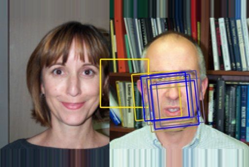
the presence of attention in the visual cortex [9, 10]. Recently, in visual neuroscience, attention has
been shown to exist not only in extrastriate areas, but also all the way down to V1 [11].
Attention as a form of routing was originally proposed by Anderson and Van Essen [12] and then
extended by Olshausen et al. [13]. Dynamic routing has been hypothesized as providing a way for
achieving shift and size invariance in the visual cortex [14, 15]. Tsotsos et al. [16] proposed a model
combining search and attention called the Selective Tuning model. Larochelle and Hinton [17] pro-
posed a way of using third-order Boltzmann Machines to combine information gathered from many
foveal glimpses. Their model chooses where to look next to find locations that are most informative
of the object class. Reichert et al. [18] proposed a hierarchical model to show that certain aspects of
covert object-based attention can be modeled by Deep Boltzmann Machines. Several other related
models attempt to learn where to look for objects [19, 20] and for video based tracking [21]. Inspired
by Olshausen et al. [13], we use 2D similarity transformations to implement the scaling, rotation,
and shift operation required for routing. Our main motivation is to enable the learning of generative
models in big images where the location of the object of interest is unknown a-priori.

2       Gaussian Restricted Boltzmann Machines
Before we describe our model, we briefly review the Gaussian Restricted Boltzmann Machine
(GRBM) [22], as it will serve as the building block for our attention-based model. GRBMs are
a type of Markov Random Field model that has a bipartite structure with real-valued visible vari-
ables v ∈ RD connected to binary stochastic hidden variables h ∈ {0, 1}H . The energy of the joint
configuration {v, h} of the Gaussian RBM is defined as follows:
                                      1 X (vi − bi )2 X                X
               EGRBM (v, h; Θ) =                       −      c j hj −    Wij vi hj ,          (1)
                                      2 i       σi2        j           ij

where Θ = {W, b, c, σ}
                     P are the model parameters. The marginal distribution over the visible vector
                  1
v is P (v; Θ) = Z(Θ)    h exp (−E(v, h; Θ)) and the corresponding conditional distributions take
the following form:
                                              X
               p(hj = 1|v) = 1/ 1 + exp(−         Wij vi − cj ) ,                              (2)
                                                            i
                                                                                 X
                         p(vi |h)   = N (vi ; µi , σi2 ), where µi = bi + σi2        Wij hj .         (3)
                                                                                 j

Observe that conditioned on the states of the hidden variables (Eq. 3), each visible unit is modeled
by a Gaussian distribution, whose mean is shifted by the weighted combination of the hidden unit
activations. Unlike directed models, an RBM’s conditional distribution over hidden nodes is factorial
and can be easily computed.
We can also add a binary RBM on top of the learned GRBM by treating the inferred h as the
“visible” layer together with a second hidden layer h2 . This results in a 2-layer Gaussian Deep
Belief Network (GDBN) [1] that is a more powerful model of v.
Specifically, in a GDBN model, p(h1 , h2 ) is modeled by the energy function of the 2nd-layer RBM,
while p(v1 |h1 ) is given by Eq. 3. Efficient inference can be performed using the greedy approach
of [1] by treating each DBN layer as a separate RBM model. GDBNs have been applied to various
tasks, including image classification, video action and speech recognition [6, 23, 24, 25].

3       The Model
Let I be a high resolution image of a scene, e.g. a 256×256 image. We want to use attention to
propagate regions of interest from I up to a canonical representation. For example, in order to learn
a model of faces, the canonical representation could be a 24×24 aligned and cropped frontal face
image. Let v ∈ RD represent this low resolution canonical image. In this work, we focus on a Deep
Belief Network1 to model v.
This is illustrated in the diagrams of Fig. 1. The left panel displays the model of Olshausen et.al. [13],
whereas the right panel shows a graphical diagram of our proposed generative model with an atten-
tional mechanism. Here, h1 and h2 represent the latent hidden variables of the DBN model, and
    1
        Other generative models can also be used with our attention framework.

                                                        2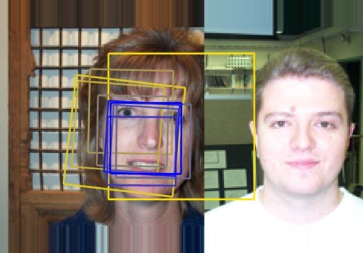
2d similarity
                                                                                    transformation

                       Olshausen et al. 93                                    Our model

Figure 1: Left: The Shifter Circuit, a well-known neuroscience model for visual attention [13]; Right: The
proposed model uses 2D similarity transformations from geometry and a Gaussian DBN to model canonical
face images. Associative memory corresponds to the DBN, object-centered frame correspond to the visible
layer and the attentional mechanism is modeled by 2D similarity transformations.

4x, 4y, 4θ, 4s (position, rotation, and scale) are the parameters of the 2D similarity transforma-
tion.
The 2D similarity transformation is used to rotate, scale, and translate the canonical image v onto the
canvas that we denote by I. Let p = [x y]T be a pixel coordinate (e.g. [0, 0] or [0, 1]) of the canonical
image v. Let {p} be the set of all coordinates of v. For example, if v is 24×24, then {p} ranges
from [0, 0] to [23, 23]. Let the “gaze” variables u ∈ R4 ≡ [4x, 4y, 4θ, 4s] be the parameter
of the Similarity transformation. In order to simplify derivations and to make transformations be
linear w.r.t. the transformation parameters, we can equivalently redefine u = [a, b, 4x, 4y],
where a = s sin(θ) − 1 and b = s cos(θ) (see [26] for details). We further define a function
w := w(p, u) → p0 as the transformation function to warp points p to p0 :
                              h 0 i h
                                x         1+a        −b        x          4x
                                                           ih     i h          i
                        p0 ,      0  =                              +           .                     (4)
                                y            b      1+a        y          4y
We use the notation I({p}) to denote the bilinear interpolation of I at coordinates {p} with anti-
aliasing. Let x(u) be the extracted low-resolution image at warped locations p0 :

                                             x(u) , I(w({p}, u)).                                     (5)
Intuitively, x(u) is a patch extracted from I according to the shift, rotation and scale parameters
of u, as shown in Fig. 1, right panel. It is this patch of data that we seek to model generatively. Note
that the dimensionality of x(u) is equal to the cardinality of {p}, where {p} denotes the set of pixel
coordinates of the canonical image v. Unlike standard generative learning tasks, the data x(u) is
not static but changes with the latent variables u. Given v and u, we model the top-down generative
process over2 x with a Gaussian distribution having a diagonal covariance matrix σ 2 I:
                                                       1 X (xi (u) − vi )2

                           p(x|v, u, I) ∝ exp −                                .                     (6)
                                                       2 i          σi2

The fact that we do not seek to model the rest of the regions/pixels of I is by design. By using 2D
similarity transformation to mimic attention, we can discard the complex background of the scene
and let the generative model focus on the object of interest. The proposed generative model takes
the following form:
                                     p(x, v, u|I) = p(x|v, u, I)p(v)p(u),                             (7)
where for p(u) we use a flat prior that is constant for all u, and p(v) is defined by a 2-layer Gaussian
Deep Belief Network. The conditional p(x|v, u, I) is given by a Gaussian distribution as in Eq. 6.
To simplify the inference procedure, p(x|v, u, I) and the GDBN model of v, p(v), will share the
same noise parameters σi .
   2
       We will often omit dependence of x on u for clarity of presentation.

                                                        3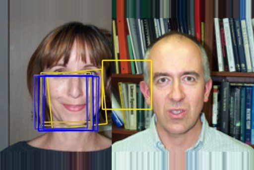
4   Inference
While the generative equations in the last section are straightforward and intuitive, inference in these
models is typically intractable due to the complicated energy landscape of the posterior. During
inference, we wish to compute the distribution over the gaze variables u and canonical object v given
the big image I. Unlike in standard RBMs and DBNs, there are no simplifying factorial assumptions
about the conditional distribution of the latent variable u. Having a 2D similarity transformation is
reminiscent of third-order Boltzmann machines with u performing top-down multiplicative gating
of the connections between v and I. It is well known that inference in these higher-order models is
rather complicated.
One way to perform inference in our model is to resort to Gibbs sampling by computing the set of
alternating conditional posteriors: The conditional distribution over the canonical image v takes the
following form:
                                                    µ + x(u)
                                p(v|u, h1 , I) = N              ; σ2 ,                            (8)
                                                          2
where µi = bi + σi2 j Wij h1j is the top-down influence of the DBN. Note that if we know the
                      P

gaze variable u and the first layer of hidden variables h1 , then v is simply defined by a Gaussian
distribution, where the mean is given by the average of the top-down influence and bottom-up in-
formation from x. The conditional distributions over h1 and h2 given v are given by the standard
DBN inference equations [1]. The conditional posterior over the gaze variables u is given by:
                              p(x|u, v)p(u)
                 p(u|x, v) =                 ,
                                  p(x|v)
                                                           1 X (xi (u) − vi )2
             log p(u|x, v) ∝ log p(x|u, v) + log p(u) =                         + const.          (9)
                                                           2 i         σi2
Using Bayes’ rule, the unnormalized log probability of p(u|x, v) is defined in Eq. 9. We stress that
this equation is atypical in that the random variable of interest u actually affects the conditioning
variable x (see Eq. 5) We can explore the gaze variables using Hamiltonian Monte Carlo (HMC)
algorithm [27, 28]. Intuitively, conditioned on the canonical object v that our model has in “mind”,
HMC searches over the entire image I to find a region x with a good match to v.
If the goal is only to find the MAP estimate of p(u|x, v), then we may want to use second-order
methods for optimizing u. This would be equivalent to the Lucas-Kanade framework in computer
vision, developed for image alignment [29]. However, HMC has the advantage of being a proper
MCMC sampler that satisfies detailed balance and fits nicely with our probabilistic framework.
The HMC algorithm first specifies the Hamiltonian over the position variables u and auxiliary
momentum variables r: H(u, r) = U (u) + K(r), where the potential function is defined by
                          2
U (u) = 21 i (xi (u)−v  i)
                             and the kinetic energy function is given by K(r) = 12 i ri2 . The dy-
           P                                                                          P
                    σi2
namics of the system is defined by:
                                      ∂u            ∂r      ∂H
                                          = r,         =−                                     (10)
                                      ∂t            ∂t       ∂u
                   ∂H       (x(u) − v) ∂x(u)
                        =                      ,                                              (11)
                   ∂u           σ2       ∂u
                   ∂x           ∂x      ∂w({p}, u) X            ∂xi      ∂w(pi , u)
                        =                            =                              .         (12)
                   ∂u       ∂w({p}, u)       ∂u          i
                                                            ∂w(p  i , u)   ∂u

Observe that Eq. 12 decomposes into sums over single coordinate positions pi = [x y]T . Let us
denote p0 i = w(pi , u) to be the coordinate pi warped by u. For the first term on the RHS of Eq. 12,

                                ∂xi
                                      = ∇I(p0 i ), (dimension 1 by 2 )                         (13)
                           ∂w(pi , u)
where ∇I(p0 i ) denotes the sampling of the gradient images of I at the warped location pi . For the
second term on the RHS of Eq. 12, we note that we can re-write Eq. 4 as:
                                                       " a #
                         h 0 i h
                            x         x −y 1 0            b           x
                                                      i            h    i
                              0   =                             +         ,                    (14)
                            y         y x 0 1            4x           y
                                                         4y

                                                   4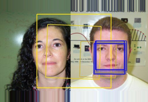
giving us
                                  ∂w(pi , u) h x        −y    1   0
                                                                    i
                                            =                        .                               (15)
                                    ∂u         y        x     0   1

HMC simulates the discretized system by performing leap-frog updates of u and r using Eq. 10.
Additional hyperparameters that need to be specified include the step size , number of leap-frog
steps, and the mass of the variables (see [28] for details).

4.1 Approximate Inference
HMC essentially performs gradient descent with momentum,
therefore it is prone to getting stuck at local optimums. This
is especially a problem for our task of finding the best trans-
formation parameters. While the posterior over u should be
unimodal near the optimum, many local minima exist away
from the global optimum. For example, in Fig. 2(a), the big
image I is enclosed by the blue box, and the canonical image
v is enclosed by the green box. The current setting of u aligns                     (a)
together the wrong eyes. However, it is hard to move the green
                                                                                       Average
box to the left due to the local optima created by the dark in-
                                                                                A
tensities of the eye. Resampling the momentum variable every
iteration in HMC does not help significantly because we are                                      B
modeling real-valued images using a Gaussian distribution as
the residual, leading to quadratic costs in the difference be-
tween x(u) and v (see Eq. 9). This makes the energy barriers
between modes extremely high.
To alleviate this problem we need to find good initializations
of u. We use a Convolutional Network (ConvNet) to per-
form efficient approximate inference, resulting in good initial               (b)
guesses. Specifically, given v, u and I, we predict the change Figure 2: (a) HMC can easily get
in u that will lead to the maximum log p(u|x, v). In other stuck at local optima. (b) Importance
words, instead of using the gradient field for updating u, we of modeling p(u|v, I). Best in color.
learn a ConvNet to output a better vector field in the space
of u. We used a fairly standard ConvNet architecture and the standard stochastic gradient descent
learning procedure.
We note that standard feedforward face detectors seek to model p(u|I), while completely ignoring
the canonical face v. In contrast, here we take v into account as well. The ConvNet is used to initial-
ize u for the HMC algorithm. This is important in a proper generative model because conditioning
on v is appealing when multiple faces are present in the scene. Fig. 2(b) is a hypothesized Euclidean
space of v, where the black manifold represents canonical faces and the blue manifold represents
cropped faces x(u). The blue manifold has a low intrinsic dimensionality of 4, spanned by u. At A
and B, the blue comes close to black manifold. This means that there are at least two modes in the
posterior over u. By conditioning on v, we can narrow the posterior to a single mode, depending on
whom we want to focus our attention. We demonstrate this exact capability in Sec. 6.3.
Fig. 3 demonstrates the iterative process of how approximate inference works in our model. Specif-
ically, based on u, the ConvNet takes a window patch around x(u) (72×72) and v (24×24) as input,
and predicts the output [4x, 4y, 4θ, 4s]. In step 2, u is updated accordingly, followed by step 3
of alternating Gibbs updates of v and h, as discussed in Sec. 4. The process is repeated. For the
details of the ConvNet see the supplementary materials.

5   Learning
While inference in our framework localizes objects of interest and is akin to object detection, it is not
the main objective. Our motivation is not to compete with state-of-the-art object detectors but rather
propose a probabilistic generative framework capable of generative modeling of objects which are
at unknown locations in big images. This is because labels are expensive to obtain and are often not
available for images in an unconstrained environment.
To learn generatively without labels we propose a simple Monte Carlo based Expectation-
Maximization algorithm. This algorithm is an unbiased estimator of the maximum likelihood objec-

                                                   5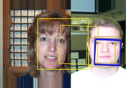
1 Gibbs step
                        ConvNet                                             ConvNet

    Step 1                        Step 2                       Step 3                 Step 4

Figure 3: Inference process: u in step 1 is randomly initialized. The average v and the extracted x(u) form
the input to a ConvNet for approximate inference, giving a new u. The new u is used to sample p(v|I, u, h).
In step 3, one step of Gibbs sampling of the GDBN is performed. Step 4 repeats the approximate inference
using the updated v and x(u).

                                           V

                                           X

                                                1        2              3        4        5          6
                                                                                               HMC
                                                         Inference steps
Figure 4: Example of an inference step. v is 24×24, x is 72×72. Approximate inference quickly finds a
good initialization for u, while HMC provides further adjustments. Intermediate inference steps on the right
are subsampled from 10 actual iterations.

tive. During the E-step, we use the Gibbs sampling algorithm developed in Sec. 4 to draw samples
from the posterior over the latent gaze variables u, the canonical variables v, and the hidden vari-
ables h1 , h2 of a Gaussian DBN model. During the M-step, we can update the weights of the
Gaussian DBN by using the posterior samples as its training data. In addition, we can update the
parameters of the ConvNet that performs approximate inference. Due to the fact that the first E-step
requires a good inference algorithm, we need to pretrain the ConvNet using labeled gaze data as
part of a bootstrap process. Obtaining training data for this initial phase is not a problem as we can
jitter/rotate/scale to create data. In Sec. 6.2, we demonstrate the ability to learn a good generative
model of face images from the CMU Multi-PIE dataset.

6    Experiments
We used two face datasets in our experiments. The first dataset is a frontal face dataset, called
the Caltech Faces from 1999, collected by Markus Weber. In this dataset, there are 450 faces of 27
unique individuals under different lighting conditions, expressions, and backgrounds. We downsam-
pled the images from their native 896 by 692 by a factor of 2. The dataset also contains manually
labeled eyes and mouth coordinates, which will serve as the gaze labels. We also used the CMU
Multi-PIE dataset [30], which contains 337 subjects, captured under 15 viewpoints and 19 illumi-
nation conditions in four recording sessions for a total of more than 750,000 images. We demon-
strate our model’s ability to perform approximate inference, to learn without labels, and to perform
identity-based attention given an image with two people.
6.1 Approximate inference
We first investigate the critical inference algorithm of p(u|v, I) on the Caltech Faces dataset. We
run 4 steps of approximate inference detailed in Sec. 4.1 and diagrammed in Fig. 3, followed by
three iterations of 20 leap-frog steps of HMC. Since we do not initially know the correct v, we
initialize v to be the average face across all subjects.
Fig. 4 shows the image of v and x during inference for a test subject. The initial gaze box is colored
yellow on the left. Subsequent gaze updates progress from yellow to blue. Once ConvNet-based
approximate inference gives a good initialization, starting from step 5, five iterations of 20 leap-frog
steps of HMC are used to sample from the the posterior.
Fig. 5 shows the quantitative results of Intersection over Union (IOU) of the ground truth face box
and the inferred face box. The results show that inference is very robust to initialization and requires

                                                     6
Accuracy of Approximate Inference                      Accuracy of Approximate Inference                             Accuracy Improvements
           1.1                                                                                                            0.3
                                                                   1                                                                      Average IOU Improvements
            1                                                                                                             0.2
                                                                  0.8
Accuracy

                                                       Accuracy

                                                                                                              Accuracy
           0.9
                                                                                                                          0.1
                                                                  0.6
           0.8
                                                                                                                           0
           0.7                                                    0.4
                    Trials with IOU > 0.5                                        Trials with IOU > 0.5
           0.6                                                    0.2                                                    −0.1
                    Average IOU                                                  Average IOU

           0.5                                                     0                                                     −0.2
              0     20      40      60      80   100                0        5               10          15                  0   20       40    60     80    100
                         Initial Pixel Offset                            # of Inference Steps                                         Initial Pixel Offset
                 (a)                                  (b)                                     (c)
Figure 5: (a) Accuracy as a function of gaze initialization (pixel offset). Blue curve is the percentage success
of at least 50% IOU. Red curve is the average IOU. (b) Accuracy as a function of the number of approximate
inference steps when initializing 50 pixels away. (c) Accuracy improvements of HMC as a function of gaze
initializations.

                                     (a) DBN trained on Caltech                              (b) DBN updated with Multi-PIE
Figure 6: Left: Samples from a 2-layer DBN trained on Caltech. Right: samples from an updated DBN after
training on CMU Multi-PIE without labels. Samples highlighted in green are similar to faces from CMU.

only a few steps of approximate inference to converge. HMC clearly improves model performance,
resulting in an IOU increase of about 5% for localization. This is impressive given that none of
the test subjects were part of the training and the background is different from backgrounds in the
training set.
                                                         We also compared our inference algorithm to
               Our method OpenCV NCC template            the template matching in the task of face de-
  IOU > 0.5       97%        97%       93%       78%     tection. We took the first 5 subjects as test
 # evaluations    O(c)     O(whs) O(whs) O(whs)          subjects and the rest as training. We can lo-
Table 1: Face localization accuracy. w: image width; calize with 97% accuracy 3(IOU > 0.5) us-
h: image height; s: image scales; c: number of inference ing our inference algorithm . In comparison,
steps used.                                              a near state-of-the-art face detection system
                                                         from OpenCV 2.4.9 obtains the same 97% ac-
curacy. It uses Haar Cascades, which is a form of AdaBoost4 . Normalized Cross Correlation [31]
obtained 93% accuracy, while Euclidean distance template matching achieved an accuracy of only
78%. However, note that our algorithm looks at a constant number of windows while the other
baselines are all based on scanning windows.
6.2               Generative learning without labels
                nats     No CMU training CMU w/o labels CMU w/ labels
                                                                     The main advantage of our
           Caltech Train    617±0.4        627±0.5        569±0.6    model is that it can learn on
           Caltech Valid    512±1.1        503±1.8        494±1.7    large images of faces without lo-
            CMU Train        96±0.8        499±0.1        594±0.5    calization label information (no
            CMU Valid        85±0.5        387±0.3        503±0.7    manual cropping required). To
               log Ẑ         454.6         687.8          694.2     demonstrate, we use both the
                                                                     Caltech and the CMU faces
Table 2: Variational lower-bound estimates on the log-density of the dataset. For the CMU faces, a
Gaussian DBNs (higher is better).
                                                                     subset of 2526 frontal faces with
ground truth labels are used. We split the Caltech dataset into a training and a validation set. For
the CMU faces, we first took 10% of the images as training cases for the ConvNet for approximate
inference. This is needed due to the completely different backgrounds of the Caltech and CMU
datasets. The remaining 90% of the CMU faces are split into a training and validation set. We first
trained a GDBN with 1024 h1 and 256 h2 hidden units on the Caltech training set. We also trained
             3
   u is randomly initialized at ± 30 pixels, scale range from 0.5 to 1.5.
             4
   OpenCV detection uses pretrained model from haarcascade_frontalface_default.xml, scaleFactor=1.1,
minNeighbors=3 and minSize=30.

                                                                                     7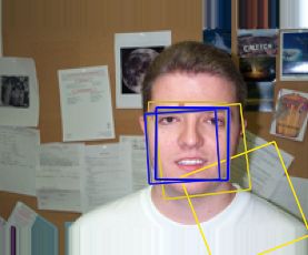
Figure 7: Left: Conditioned on different v will result in a different 4u. Note that the initial u is exactly the
same for two trials. Right: Additional examples. The only difference between the top and bottom panels is the
conditioned v. Best viewed in color.

a ConvNet for approximate inference using the Caltech training set and 10% of the CMU training
images.
Table 2 shows the estimates of the variational lower-bounds on the average log-density (higher is
better) that the GDBN models assign to the ground-truth cropped face images from the training/test
sets under different scenarios. In the left column, the model is only trained on Caltech faces. Thus it
gives very low probabilities to the CMU faces. Indeed, GDBNs achieve a variational lower-bound of
only 85 nats per test image. In the middle column, we use our approximate inference to estimate the
location of the CMU training faces and further trained the GDBN on the newly localized faces. This
gives a dramatic increase of the model performance on the CMU Validation set5 , achieving a lower-
bound of 387 nats per test image. The right column gives the best possible results if we can train
with the CMU manual localization labels. In this case, GDBNs achieve a lower-bound of 503 nats.
We used Annealed Importance Sampling (AIS) to estimate the partition function for the top-layer
RBM. Details on estimating the variational lower bound are in the supplementary materials.
Fig. 6(a) further shows samples drawn from the Caltech trained DBN, whereas Fig. 6(b) shows
samples after training with the CMU dataset using estimated u. Observe that samples in Fig. 6(b)
show a more diverse set of faces. We trained GDBNs using a greedy, layer-wise algorithm of [1].
For the top layer we use Fast Persistent Contrastive Divergence [32], which substantially improved
generative performance of GDBNs (see supplementary material for more details).
6.3 Inference with ambiguity
Our attentional mechanism can also be useful when multiple objects/faces are present in the scene.
Indeed, the posterior p(u|x, v) is conditioned on v, which means that where to attend is a func-
tion of the canonical object v the model has in “mind” (see Fig. 2(b)). To explore this, we first
synthetically generate a dataset by concatenating together two faces from the Caltech dataset. We
then train approximate inference ConvNet as in Sec. 4.1 and test on the held-out subjects. Indeed,
as predicted, Fig. 7 shows that depending on which canonical image is conditioned, the same exact
gaze initialization leads to two very different gaze shifts. Note that this phenomenon is observed
across different scales and location of the initial gaze. For example, in Fig. 7, right-bottom panel,
the initialized yellow box is mostly on the female’s face to the left, but because the conditioned
canonical face v is that of the right male, attention is shifted to the right.
7    Conclusion
In this paper we have proposed a probabilistic graphical model framework for learning generative
models using attention. Experiments on face modeling have shown that ConvNet based approximate
inference combined with HMC sampling is sufficient to explore the complicated posterior distribu-
tion. More importantly, we can generatively learn objects of interest from novel big images. Future
work will include experimenting with faces as well as other objects in a large scene. Currently the
ConvNet approximate inference is trained in a supervised manner, but reinforcement learning could
also be used instead.
Acknowledgements
The authors gratefully acknowledge the support and generosity from Samsung, Google, and ONR
grant N00014-14-1-0232.
   5
     We note that we still made use of labels coming from the 10% of CMU Multi-PIE training set in order to
pretrain our ConvNet. "w/o labels" here means that no labels for the CMU Train/Valid images are given.

                                                       8
References
 [1] G. E. Hinton, S. Osindero, and Y. W. Teh. A fast learning algorithm for deep belief nets. Neural Compu-
     tation, 18(7):1527–1554, 2006.
 [2] R. Salakhutdinov and G. Hinton. Deep Boltzmann machines. In AISTATS, 2009.
 [3] Geoffrey E. Hinton, Peter Dayan, and Michael Revow. Modeling the manifolds of images of handwritten
     digits. IEEE Transactions on Neural Networks, 8(1):65–74, 1997.
 [4] Daniel Zoran and Yair Weiss. From learning models of natural image patches to whole image restoration.
     In ICCV. IEEE, 2011.
 [5] Yoshua Bengio, Li Yao, Guillaume Alain, and Pascal Vincent. Generalized denoising auto-encoders as
     generative models. In Advances in Neural Information Processing Systems 26, 2013.
 [6] H. Lee, R. Grosse, R. Ranganath, and A. Y. Ng. Convolutional deep belief networks for scalable unsu-
     pervised learning of hierarchical representations. In ICML, pages 609–616, 2009.
 [7] Marc’Aurelio Ranzato, Joshua Susskind, Volodymyr Mnih, and Geoffrey Hinton. On Deep Generative
     Models with Applications to Recognition. In CVPR, 2011.
 [8] Yichuan Tang, Ruslan Salakhutdinov, and Geoffrey E. Hinton. Deep mixtures of factor analysers. In
     ICML. icml.cc / Omnipress, 2012.
 [9] M. I. Posner and C. D. Gilbert. Attention and primary visual cortex. Proc. of the National Academy of
     Sciences, 96(6), March 1999.
[10] E. A. Buffalo, P. Fries, R. Landman, H. Liang, and R. Desimone. A backward progression of attentional
     effects in the ventral stream. PNAS, 107(1):361–365, Jan. 2010.
[11] N Kanwisher and E Wojciulik. Visual attention: Insights from brain imaging. Nature Reviews Neuro-
     science, 1:91–100, 2000.
[12] C. H. Anderson and D. C. Van Essen. Shifter circuits: A computational strategy for dynamic aspects of
     visual processing. National Academy of Sciences, 84:6297–6301, 1987.
[13] B. A. Olshausen, C. H. Anderson, and D. C. Van Essen. A neurobiological model of visual attention and
     invariant pattern recognition based on dynamic routing of information. The Journal of neuroscience : the
     official journal of the Society for Neuroscience, 13(11):4700–4719, 1993.
[14] Laurenz Wiskott. How does our visual system achieve shift and size invariance?, 2004.
[15] S. Chikkerur, T. Serre, C. Tan, and T. Poggio. What and where: a Bayesian inference theory of attention.
     Vision Research, 50(22):2233–2247, October 2010.
[16] J. K. Tsotsos, S. M. Culhane, W. Y. K. Wai, Y. H. Lai, N. Davis, and F. Nuflo. Modeling visual-attention
     via selective tuning. Artificial Intelligence, 78(1-2):507–545, October 1995.
[17] Hugo Larochelle and Geoffrey E. Hinton. Learning to combine foveal glimpses with a third-order boltz-
     mann machine. In NIPS, pages 1243–1251. Curran Associates, Inc., 2010.
[18] D. P. Reichert, P. Seriès, and A. J. Storkey. A hierarchical generative model of recurrent object-based
     attention in the visual cortex. In ICANN (1), volume 6791, pages 18–25. Springer, 2011.
[19] B. Alexe, N. Heess, Y. W. Teh, and V. Ferrari. Searching for objects driven by context. In NIPS 2012,
     December 2012.
[20] Marc’Aurelio Ranzato. On learning where to look. arXiv, arXiv:1405.5488, 2014.
[21] M. Denil, L. Bazzani, H. Larochelle, and N. de Freitas. Learning where to attend with deep architectures
     for image tracking. Neural Computation, 28:2151–2184, 2012.
[22] G. E. Hinton and R. Salakhutdinov. Reducing the dimensionality of data with neural networks. Science,
     313:504–507, 2006.
[23] A. Krizhevsky. Learning multiple layers of features from tiny images, 2009.
[24] Graham W. Taylor, Rob Fergus, Yann LeCun, and Christoph Bregler. Convolutional learning of spatio-
     temporal features. In ECCV 2010. Springer, 2010.
[25] A. Mohamed, G. Dahl, and G. Hinton. Acoustic modeling using deep belief networks. IEEE Transactions
     on Audio, Speech, and Language Processing, 2011.
[26] Richard Szeliski. Computer Vision - Algorithms and Applications. Texts in Computer Science. Springer,
     2011.
[27] S. Duane, A. D. Kennedy, B. J Pendleton, and D. Roweth. Hybrid Monte Carlo. Physics Letters B,
     195(2):216–222, 1987.
[28] R. M. Neal. MCMC using Hamiltonian dynamics. in Handbook of Markov Chain Monte Carlo (eds S.
     Brooks, A. Gelman, G. Jones, XL Meng). Chapman and Hall/CRC Press, 2010.
[29] Simon Baker and Iain Matthews. Lucas-kanade 20 years on: A unifying framework. International Journal
     of Computer Vision, 56:221–255, 2002.
[30] Ralph Gross, Iain Matthews, Jeffrey F. Cohn, Takeo Kanade, and Simon Baker. Multi-pie. Image Vision
     Comput., 28(5):807–813, 2010.
[31] J. P. Lewis. Fast normalized cross-correlation, 1995.
[32] T. Tieleman and G. E. Hinton. Using fast weights to improve persistent contrastive divergence. In ICML,
     volume 382, page 130. ACM, 2009.
[33] R. Salakhutdinov and I. Murray. On the quantitative analysis of deep belief networks. In Proceedings of
     the Intl. Conf. on Machine Learning, volume 25, 2008.

                                                     9
You can also read