On Differences between Deterministic and Stochastic Models of Chemical Reactions: Schlögl Solved with ZI-Closure - MDPI
←
→
Page content transcription
If your browser does not render page correctly, please read the page content below
entropy
Article
On Differences between Deterministic and Stochastic
Models of Chemical Reactions: Schlögl Solved
with ZI-Closure
Michail Vlysidis and Yiannis N. Kaznessis *
 Department of Chemical Engineering and Materials Science, University of Minnesota,
 Minneapolis, MN 55455, USA; vlysi001@umn.edu
 * Correspondence: yiannis@umn.edu

 Received: 3 July 2018; Accepted: 4 September 2018; Published: 6 September 2018

 Abstract: Deterministic and stochastic models of chemical reaction kinetics can give starkly different
 results when the deterministic model exhibits more than one stable solution. For example, in the
 stochastic Schlögl model, the bimodal stationary probability distribution collapses to a unimodal
 distribution when the system size increases, even for kinetic constant values that result in two distinct
 stable solutions in the deterministic Schlögl model. Using zero-information (ZI) closure scheme,
 an algorithm for solving chemical master equations, we compute stationary probability distributions
 for varying system sizes of the Schlögl model. With ZI-closure, system sizes can be studied that
 have been previously unattainable by stochastic simulation algorithms. We observe and quantify
 paradoxical discrepancies between stochastic and deterministic models and explain this behavior by
 postulating that the entropy of non-equilibrium steady states (NESS) is maximum.

 Keywords: closure scheme; maximum entropy; non-equilibrium steady state; Schlögl

1. Background
     Chemical reaction kinetics have been canonically modeled with ordinary differential equations
since the pronouncement of the law of mass action kinetics, 150 years ago [1]. This macroscopic,
continuous-deterministic modeling formalism is appropriate at the thermodynamic limit, when the
volume of the system and the numbers of molecules of reactants all tend to very large values.
     Markov chain models can be used for chemical reactions away from the thermodynamic limit [2].
Models are then formulated in terms of discrete numbers of molecules for each of the chemical species
present at time t. The system evolves stochastically, and the all-encompassing chemical master equation
(CME) can model the probability distribution of the system being at a particular state at time t [3].
     Kurtz [4,5] explored the relationship between stochastic and deterministic models when the
macroscopic equations have a unique, asymptotically stable solution, and demonstrated that the
deterministic model is the thermodynamic limit of the stochastic one.
     However, when the ordinary differential equations admit more than one stable solutions, the two
formalisms may give starkly different results for even simple, small chemical reaction models [6–9].
The Schlögl model is such a simple model [10], described as follows [11]:

                                               k1                k3
                                           3X*
                                             )2 X + A         X*
                                                               ) B.
                                               k02               k04

     This is a one-dimensional model. The only variable is the number of molecules X. Species A and
B are present in the system with constant concentrations, arriving from separate external reservoirs.
Setting k2 = k02 [ A] and k4 = k04 [ B], the model is simplified as

Entropy 2018, 20, 678; doi:10.3390/e20090678                                  www.mdpi.com/journal/entropy
Entropy 2018, 20, 678 2 of 14
1 k k3
3X*
)2 X ) ∅.
X*
k2 k4
For a large system of volume V, the concentration x = X/V changes in time according to the law
of mass action,
dx
= −k1 x3 + k2 x2 − k3 x + k4 . (1)
dt
This cubic equation admits either a single stable solution, or two stable solutions and one unstable
one [12]. The solution depends on kinetic constant and reservoir concentration values. Herein we
retain values of all kinetic parameters constant, except k4 . The values of the constant kinetic parameters
are (k1 , k2 , k3 ) = (0.42, 70, 3150). We present results for k4 ranging from 104 to 7 × 10⁴ .
The chemical master equation for the Schlögl model has been formulated before [2,12,13]:
k2
∂
∂t p ( X; t ) = − 1)( X − 2) + k4 V p( X − 1; t)
V (X
− kV2 X ( X − 1) + k4 V p( X; t)
k1
+ V 2 ( X + 1) X ( X − 1) + k3 ( X + 1) p( X + 1; t)
k1
− V 2 X ( X − 1)( X − 2) + k3 X p( X; t). (2)
As discussed previously [14], for small system sizes the stationary probability distribution
p( X; t) is either unimodal or bimodal, depending on parameter values. Difficulties in computing
the stationary probability distribution for mesoscopic systems, which are still under the influence of
molecular fluctuations, but have molecular populations too large for stochastic simulation algorithms,
have hampered the analysis of stationary probability distributions.
Herein we solve the master equation using ZI-closure scheme [14] for large system sizes that were
previously unattainable with other methods. We keep the concentration x constant, while systematically
increasing the system size, in order to investigate the collapse of bimodality for mesoscopic and large
systems, and determine the limits of correspondence between CME and ODE models.
Please note that the systems studied in this work are not at equilibrium. The chemical potentials
of the two reservoirs in the Schlögl reaction are set to be different. There is then mass flowing from the
reservoir with high chemical potential to the reservoir with low chemical potential. The flow of mass
is at steady state, and as a result the probability distribution of X within the system is stationary.
By varying the kinetic constants, the steady state changes. We study the stationary probability
distribution of these non-equilibrium steady states (NESS). NESS is one of three types of dynamics
observed in chemical reaction systems [12]: (a) equilibrium state with fluctuations as described by
classical statistical mechanics theories, (b) time-dependent, transient processes in which the state of
systems changes with time, and (c) NESS [15].
We study the Schlögl model as a simple example of a bistable system. This model has been used
extensively to model physical and chemical systems [16–24]. There is also a plethora of biological
systems exhibiting bistability, such as the lysis and lysogeny system in phage [25]. Over the past two
decades, there has been particular interest in both synthetic and natural biological systems exhibiting
either temporal or spatial bistability [25–30]. The Schlögl model has been recognized as one of the
simplest models that can capture essential elements of bistable behavior [31]. In principle, insights
gained from studying this model can be applied to other bistable stochastic chemical reaction networks.
We also note that there a plethora of alternative, approximate numerical methods to solve
stochastic reaction systems. The goal of the current manuscript is not to provide an exhaustive review
of the literature, but we bring to the attention of the reader the following important references that
describe Fokker-Planck, Linear-Noise and moment-closure approximations [32–34].Entropy 2018, 20, 678 3 of 14
2. Zero-Information Closure Scheme
In this section, we briefly discuss the elements of the ZI-closure scheme. More details on the
method can be found in [14,35,36].
Instead of attempting to solve directly the CME, an impossible task for all but the simplest of
reaction networks, one can generate a set of ODEs that describe the time dynamics of the probability
distribution moments [37,38]. The CME for the Schlögl model can be transformed in moment equations
with the use of Z-transform of the probability distribution [38]:
∞
G (Φ, t) = ∑ Φ X p( X, t), (3)
X =0
where Φ is a new variable. Using derivatives of G w.r.t. Φ and t, the CME can be transformed into
a set of moment equations:
dµ
= Aµ + A0 µ0 + µ0 , (4)
dt
where µ is the vector of lower-order moments, µ0 is the vector of higher-order probability moments
and µ0 a constant vector representing the zero-order moment.
Herein, moments are defined as expected values of the probability distribution:
∞
X!
{Xm } = ∑ ( X − m)!
p( X, t), (5)
X =0
where { X m } is the mth factorial moment of the probability distribution.
For example, the first four moment equations for the Schlögl are calculated as:
k2
− Vk12
−k3
{X} V 0 {X}
d { X 2 } 2k4 V 4 V2 − 2k3
k
2 kV2 − 4 Vk12 −2 Vk12 { X 2 }
3 =
dt { X } 0 6 kV2 + 3k4 V −6 Vk12 − 3k3 3 kV2 − 12k4 V { X 3 }
{X4 } 0 0 24 kV2 + 4k4 V 24 kV2 − 24 Vk12 − 4k3 {X4 }
0 0 " # k4 V
0 0 {X5 }
0
+ + (6)
k1 6
−3 V 2 0 {X } 0
4 kV2 − 24 Vk12 −4 Vk12 0
For the Schlögl model, we have empirically found that at least ten moments are needed to
accurately capture the probability distribution, especially when it is bimodal [37–39].
The dependence of the lower-order vector µ = [{ X } { X 2 } { X 3 } { X 4 }] T on the higher-order one
0
µ = [{ X 5 } { X 6 }] T is evident in this equation. This is the closure scheme challenge, which we have
previously solved by developing the ZI-closure scheme [14,35,36].
For a steady state, the left-hand side of the moment equation is zero. To solve these equations,
we postulate that the probability distribution attained by the system is the one that maximizes the
entropy [40], which is given by the equation:
S = − ∑ p( X ) ln p( X ). (7)
X
Using the method of Lagrange multipliers, the probability distribution p( X ) can then be
expressed as:
Ψ
" #
X!
p( X ) = exp − ∑ λi , (8)
i =0
( X − i )!Entropy 2018, 20, 678 4 of 14
where λi is the Lagrange multiplier associated with the lower-order moment µi and Ψ represents the
size of vector µ.
The moments are related to Lagrange multipliers through Equations (5) and (8). Consequently,
an important feature of the ZI-closure scheme algorithm is that Equation (6) depends only on the
Lagrange multipliers. For a finite, explicitly defined state space, the sums in Equation (7) can be
considered explicitly. We then use a root-finding method (e.g., Newton-Raphson) to calculate the
Lagrange multipliers. The stationary probability distribution is finally directly calculated [14].
An advantage of ZI-closure over stochastic simulation algorithms is that it calculates steady state
probability distributions directly, without resorting to simulations in time. Stochastic simulations
must start with a specific initial condition in time for an ensemble of trajectories. Each trajectory can
eventually reach a steady state. Instead, ZI-closure algorithm is initiated with a specific initial guess
for the stationary probability distribution (e.g., a delta function) and numerically converges to the
steady-state p( X ).
3. Results
In this section we present results obtained with ZI-closure scheme for the stochastic Schlögl model.
3.1. Bimodality Collapse for Mesoscopic Systems
In Figure 1a, steady state probability distributions, p( x ), are plotted for a range of values of k4 .
7
Stable Deterministic Solution
Unstable Deterministic Solution
6
5
104 k4
4
3
2
1
0 50 100 150
x
(a) (b)
Figure 1. The figure shows the effect of kinetic constant k4 on the stationary probability distribution for
small systems with V = 1. (a) shows the behavior of the stochastic system. Darker areas present higher
probability. As the kinetic constant increases, the system transitions from a unimodal distribution
to a bimodal and then back to a unimodal one. (b) shows the behavior of the deterministic system.
Solid lines represent the stable deterministic solutions and the dashed-dotted line represents the
unstable solution of the ODE model. The other kinetic constants are: (k1 , k2 , k3 ) = (0.42, 70, 3150).
In accordance with the conclusion drawn by Kurtz, when the probability distribution is unimodal,
the average of X corresponds to the single stable ODE solution. This is shown in the Figure 1b,
where the ODE solution has been plotted on the x-k4 plane. We also observe that when the distribution
is bimodal, the peaks correspond to the two stable deterministic attractors (Figure 1). A main purpose
of this article is to explore deviations from this congruency, as the system size varies.
In the rest of the document, the terms “probability peak (peak)” and “attractor” will be used
interchangeably. When the intention is to draw attention to the probability distribution and focus on
the stochastic behavior the term “peak” is preferable. On the other hand, when the intention is to
compare the results of the deterministic and stochastic models, we will prefer the term “attractor”,
which pertains to both modeling formalisms.
Parenthetically, it is interesting to note that the range of k4 values where the stochastic model
exhibits bimodality does not precisely correspond to the range of k4 values where the deterministic
model exhibits bistability. The reason for this minor discrepancy is that in the ODE model (Equation (1))Entropy 2018, 20, 678 5 of 14
higher order reactions are represented in terms of X 2 and X 3 , whereas in the CME (Equation (2)),
there are X ( X − 1), ( X − 1)( X − 2), ( X + 1) X ( X − 1) and X ( X − 1)( X − 2) terms.
When the system is bistable, only one of the solutions will be reached in finite time in the ODE
model. Which one of the solutions will be reached depends on the initial conditions. In contrast,
the stochastic model is ergodic and explores the entire state space (all the possible numbers of
molecules of X) with a frequency proportional to the probability, visiting both attractors, regardless of
initial conditions.
In other words, the stochastic model identifies and distinguishes all solution attractors, whereas
the ODE model cannot. This is in accord with, among others, the study of Ge and Qian [41],
who concluded that although deterministic differential equations can define numerous attractors,
they provide no information on the relative probabilities between them. Only stochastic model
solutions can provide such insight.
What is intriguing is that as the system size increases, the stochastic Schlögl model behavior
ceases to correspond to the ODE one. The deterministic model solution is not dependent on the size of
the system and will always exhibit the same bistable behavior, for certain ranges of parameter values.
In the stochastic model, the size of the system plays a critical role. As the size increases, the bimodality
can be destroyed, at least in numerical terms, and the stationary probability distribution can become
a delta-like function, as observed previously [6,7,9,10,42–44].
This behavior is observed in Figures 2 and 3, where the stationary probability distribution is
shown as a function of the volume for two values of k4 . Both k4 values are within the range that
produces two stable solutions for Equation (1). For small volumes, the stochastic model stationary
probability distribution exhibits bimodality. The peaks then approximately correspond to the ODE
solutions (Figures 2a and 3a). We note again that this type of behavior was observed before, e.g., in [9].
As the volume increases, the model’s bimodality apparently disappears, with only one peak
remaining significant (in numerical terms, the size of the second peak is lower than the numerical,
computer accuracy). The disappearance of bimodality occurs gradually with the system size, as one of
the peaks becomes progressively smaller. Even though the less dominant peak might still exist in finite
volumes, we find that peak sizes fall below computer round-off errors. We speculate then that at the
thermodynamic limit only one peak survives. Not unexpectedly, as the volume increases, probability
distribution standard deviations decrease, resulting in a delta function centered at one of the ODE
solutions (Figures 2b and 3b). In other words for large system sizes, the stochastic model reaches only
one solution whereas the ODE model can have three solutions, two stable and one unstable.
Because of system size models previously unattainable with stochastic simulations and because of
the unexpected results, we have taken pains in ensuring the convergence and accuracy of the ZI-closure
scheme results presented herein. The reader is directed to the appendix for more information about
the accuracy of ZI-closure results. There are three ways to increase confidence in ZI-closure results:
First, in principle, for stochastic systems that satisfy the ergodic hypothesis, the CME solution does
not depend on initial conditions. In practice, we have validated this hypothesis by determining CME
solutions with the ZI-closure scheme, numerically starting with various initial probability distribution
solutions (prescribed in the initial values of the Lagrange multipliers in the numerical scheme).
Second, ZI-closure solutions of the CME are verified by the analytical expressions available for
the Schlögl model [2,43]. We note that even though the analytical solution is available, the numerical
implementation becomes impractical for large volumes because of numerical range limitations in the
calculation of the probability at X = 0 (Appendix A). For the kinetic constant of Figure 2 (k4 = 3.5 × 10⁴ )
and Figure 3 (k4 = 4 × 10⁴ ), the analytical solution fails to produce results for volume values larger
than V = 58 and V = 45, respectively.
Finally, ZI-closure solutions is verified by comparison to the probability distribution obtained
from stochastic simulation algorithm (SSA) simulations [45].Entropy 2018, 20, 678 6 of 14
Vol = 1 Vol = 10000
0.06
k4 = 3.5 104 1 k4 = 3.5 104
Probability ZI-Closure 0.8 ZI-Closure
Probability
0.04 Stable Deterministic Stable Deterministic
0.6
0.4
0.02
0.2
0 0
0 20 40 60 80 100 120 140 160 180 0 20 40 60 80 100 120 140 160 180
x x
(a) (b)
k4 = 3.5 104
1
Probability
0.5
0
10000
150
5000 100
50
0 0
Volume x
(c)
Figure 2. The probability distributions are shown for different volumes, for k4 = 3.5 × 10⁴ (c).
The system starts with bimodal distributions at small volumes (a). Bimodality collapses as the system
size increases. The stochastic model attains only one of the two deterministic solutions as the volumes
increases (b). The solid vertical lines represent the stable deterministic solutions. (c) has 220 plotted
probability distributions computed with ZI-closure.
Vol = 1 Vol = 10000
0.025
k4 = 4 104 0.8 k4 = 4 104
0.02 ZI-Closure ZI-Closure
0.6
Probability
Probability
Stable Deterministic Stable Deterministic
0.015
0.4
0.01
0.005 0.2
0 0
0 20 40 60 80 100 120 140 160 180 0 20 40 60 80 100 120 140 160 180
x x
(a) (b)
k4 = 4 104
Probability
0.6
0.4
0.2
0
10000
5000 150
100
Volume 50
0 0
x
(c)
Figure 3. Similar results to Figure 2, however here k4 = 4.0 × 10⁴ . Bimodality collapses as the system
size increases as well (a). However in this case, the stochastic model attains a different deterministic
attractor as the volumes increases (b) compared to Figure 2. The solid vertical lines represent the stable
deterministic solutions and (c) has 220 plotted probability distributions computed with ZI-closure.Entropy 2018, 20, 678 7 of 14
In light of the bimodality collapse results, it is interesting to conduct SSA simulations with
trajectories that start at one of the ODE solutions. We observe all trajectories moving to the attractor
that is attained by ZI-closure, regardless of initial conditions. Surprisingly, system trajectories quickly
transition to the stationary attractor, even if they are initiated at the second attractor (Figure 4).
This behavior is counterintuitive, especially in light of the deterministic model solutions, where the
steady state is attained that is closest to the initial conditions of a simulation.
V = 10 V = 20
125
100 k4 = 3.5 104
100
80
75
60
x
x
50
40 k4 = 4 104
25
20
0
0 20 40 60 80 100 10 20 30 40 50 60 70 80 90 100
t t
(a) (b)
Figure 4. Sample SSA trajectories for two different kinetic constants ((a): k4 = 3.5 × 10⁴ and (b):
k4 = 4 × 10⁴ ). Even though trajectories start from a different attractor, they transition to the stochastic
stationary one. As in Figure 1, x is the concentration X/V. For visual clarity, the figure presents only
a random sample of 500,000 simulated trajectories, all of which behave in a similar fashion.
A quantity that has been used to explain the collapse of bimodality in the Schlögl probability
distribution for mesoscopic systems is the passage or transition time. Mean (first) passage times can be
calculated in a single-step, one-dimensional Markov chain with a bimodal distribution. They represent
the time that is required for the system to move from one peak to the other and can be calculated from
the following formulas [2]:
c −1 x c ∞
1 1
Tac = ∑ W+ ( x ) p( x ) ∑ p(y) Tca = ∑ W− ( x ) p( x ) ∑ p ( y ), (9)
x=a y =0 x = a +1 y= x
where, Tac is the mean passage time for moving from the left peak (a) to the right (c) and Tca the
time for moving from the right to the left, at steady state. W+ ( X ) = kV2 ( X )( X − 1) + k4 V and W− ( X )
= Vk12 X ( X − 1)( X − 2) + k3 X are the transition rates.
By calculating the mean passage time for different volumes (Figure 5), it is observed that the
time moving from the right peak to the left over the time that it takes from left to right increases
exponentially. The results support previous findings [8]. Even though a second peak might exist in
higher volumes, it is significantly less important than the dominant one. Again, this implies that only
one peak may be recovered at the thermodynamic limit.
200
k4 = 4 104
150
ln (Tca/Tac)
100
50
0
0.5 1 1.5 2 2.5 3 3.5 4 4.5
V
Figure 5. The figure shows the ratio of the time required to transition from the right peak to the left one
over the time to move from the left to the right. This ratio increases exponentially with the system volume
at steady state. In this figure, results for only one kinetic constant value (k4 = 4 × 10⁴ ) are presented.Entropy 2018, 20, 678 8 of 14
3.2. Entropy of NESS Systems
ZI-closure postulates that a stochastic reaction system reaches the stationary probability distribution
that maximizes the system’s entropy.
We next study how the entropy of NESS systems changes with the volume and with k4 . We vary
V and k4 and compute the stationary distribution for each set of parameters. Each NESS has a single
entropy value.
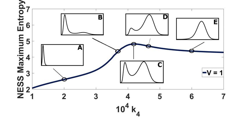
In Figure 6, the entropy of computed NESS is plotted for 600 different values of k4 at volume
V = 1. Please note that with so many points, there is the appearance of a continuous line in the graph.
At small kinetic constant values, the stationary probability distribution is unimodal (Figure 6A),
with the peak being centered at the sole stable attractor of the deterministic model, located on the
left-hand side of the state space. In this region of k4 values, the entropy of the system increases linearly
with increasing k4 .
At a certain value of k4 , the ODE will yield three solutions. The stationary probability distribution
becomes bimodal at that point, with the peak on the left attractor being dominant. The entropy of
bimodal NESS continues increasing linearly with k4 , albeit with a larger slope.
At a critical k4 value, NESS entropy reaches a maximum. At this critical value, the stationary
distribution peaks have approximately the same probability (Figure 6C).
As k4 is increased more, the probability distribution maintains its bimodal shape, but with the
right peak dominating (Figure 6D). The entropy of the system begins to decrease with k4 . Again,
at a certain value of k4 , the probability distribution becomes unimodal (Figure 6E), with the peak
located at the right hand side of the state space, resulting in another slope change.
Figure 6. NESS entropy for varying kinetic constant (k4 ) values at V = 1. Example stationary probability
distributions are depicted, as insets, to indicate the five distinct trends of NESS entropy with k4 .
The corresponding kinetic values are: k4 = 2 × 10⁴ (A), k4 = 3.7 × 10⁴ (B), k4 = 4.21 × 10⁴ (C),
k4 = 4.5 × 10⁴ (D) and k4 = 6 × 10⁴ (E).
In Figure 7, we present the NESS entropy as a function of k4 for four different system sizes,
varying the volume by 50. Again 600 NESS probability distributions are computed for different k4
values at each volume, and their entropies are plotted in this graph.
The bimodal region of the system for each volume is located between the two slope changes.
As the volume increases, the range of k4 values resulting in bimodal stationary probability distribution
decreases. This leads us to speculate that at the thermodynamic limit, the bimodal region may consist
of a single critical k4 value. At this point, the probability distribution will have two equally weighted,
distinct peaks with a total entropy of −ln (0.5).Entropy 2018, 20, 678 9 of 14
NESS Maximum Entropy
5
4
3
2 V=1
V=5
1 V = 10
V = 50
0
1 2 3 4 5 6 7
104 k4
Figure 7. The maximum entropy of different NESS probability distributions plotted against the
kinetic constant k4 , for four different volumes V. Each volume line includes more than 600 points, with
each one of them corresponding to a different NESS. With so many points there is the appearance of
a continuous line for each V.
4. Discussion
The differences between deterministic and stochastic models for chemical reaction networks have
long been the subject of numerous investigations [6–8]. Herein we also present results that highlight
such differences, focusing on the collapse of bimodality of the Schlögl model for mesoscopic and
macroscopic systems.
The size of the system is an important parameter. For small systems, the stochastic model produces
a bimodal stationary distribution with peaks near the ODE solutions. As the system size increases,
the stochastic model gradually prefers only one of the two attractors. Please note that the observed
destruction of bimodality is solely a numerical interpretation of the results. In other words, we observe
the one peak disappearing only in the numerical sense. It may well be the case that a second peak is
present but at a value lower than the allowable computer precision. We observe this behavior with
ZI-closure scheme solutions, with analytical solutions and with SSA trajectories.
The question then arises: what drives a mesoscopic system to only one of the two attractors?
This is especially puzzling, when the initial condition is the second attractor and both of these attractors
are stable solutions of the ODE model.
Numerous explanations have been provided for the discrepancies, including ones based on the
mean transition times between peaks [8]. In other studies, efforts were made to connect these differences
to the entropy production rate [41,43]. In fact, numerous efforts have attempted, and ultimately failed,
to establish whether a stability criterion for non-equilibrium steady states can exist based on the rate of
entropy production [43,46–50]. We remind the reader that when closed systems are at an equilibrium
state the stability criterion is that the entropy is maximum. There is no such established criterion for
non-equilibrium steady states.
In this study, NESS stationary probability distributions are reached when the entropy of the
system is maximum. We stress that the ZI-closure scheme postulates a maximum entropy for every
NESS and then computes the correct probability distribution, numerically matching the ones from
kinetic Monte Carlo simulations and the analytical solution. In other words, the solution of the CME
obtained by ZI-closure scheme is the probability distribution with maximum entropy. This was also
observed previously for numerous other stochastic chemical reaction systems, including stochastic
dimerization, stochastic Michaelis-Menten and stochastic cycle reaction networks [14].
Please note that the total entropy of the system and the two reservoirs increases with time.
Given a non-zero difference between the chemical potentials of the two reservoirs, there is mass transfer
from the high to the low chemical potential reservoir. This is overall an irreversible process with
positive entropy production. Yet, within the system of interest, a stationary probability distribution
is attained, which implies that the entropy of the system contained within volume V is constant.
Additionally, for open, isothermal, isochoric systems, the relevant equilibrium thermodynamicEntropy 2018, 20, 678 10 of 14
property is the Helmholtz free energy. Herein the defined Schlögl model is void of enthalpic constraints.
Thus a minimum Helmholtz free energy is equivalent to a maximum entropy.
5. Summary
We present solutions of the CME for Schlögl model systems. The results cover a wide range of
system sizes, previously unattainable with traditional methods (e.g., SSA, analytical solution). This is
possible now with the employment of ZI-closure scheme. As reported previously, for mesoscopic
systems, the exhibited bimodality collapses and only one of the attractors becomes dominant with
probability 1.
It is revealed that the range of kinetic constant values where bimodality survives, at least in
numerical terms, diminishes in larger systems. Presumably, there is a single value of k4 where
bimodality apparently survives at the thermodynamic limit. This is only speculative because, although
the ZI-closure scheme affords the investigation of system sizes that remained inaccessible in previous
studies, it is also still limited to finite volumes.
The ZI-closure scheme postulates a maximum entropy for non-equilibrium steady states in
order to numerically close the moment equations and compute the stationary probability distribution.
We wonder whether one can argue that since the probability obtained is the correct one, it follows that
the entropy of this NESS is maximum. In other words, at a stable NESS the system will attain values
for the number of molecules of X that result in the probability distribution with a maximum entropy.
We will continue investigating whether this criterion holds generally for NESS systems.
Author Contributions: M.V. and Y.N.K. designed the study and wrote the manuscript. M.V. conducted the
simulations. Conceptualization, M.V. and Y.N.K.; Formal analysis, M.V.; Funding acquisition, Y.N.K.; Investigation,
M.V.; Methodology, M.V. and Y.N.K.; Project administration, Y.N.K.; Resources, Y.N.K.; Visualization, M.V.;
Writing—original draft, M.V. and Y.N.K.
Funding: This work was supported by the National Institutes of Health [Grant No. GM111358]; National Science
Foundation [Grant No. CBET-1412283]; Extreme Science and Engineering Discovery Environment (XSEDE)
[National Science Foundation Grant No. ACI-10535753]; Minnesota Supercomputing Institute (MSI); and the
University of Minnesota Digital Technology Center.
Acknowledgments: This paper was written in part while YNK was a Visiting Scholar at the Isaac Newton Institute
of Mathematical Sciences at the University of Cambridge.
Conflicts of Interest: The authors declare no conflict of interest.
Appendix A. ZI-Closure Accuracy
The most popular method to solve stochastic reaction networks is SSA [45]. Even though SSA is
accurate, it is computationally expensive. As a result, SSA is often impractical for parametric analysis.
For example, for the Schlögl model for the kinetic parameters reported earlier and volume V = 3,
SSA needs more than 1500 CPU hours to reach steady state for a simulation with 105 trajectories.
In comparison, ZI-closure scheme for the same system needs only 2 CPU seconds. We have previously
presented comparisons between ZI-closure and SSA for several chemical reaction networks, including
Schlögl [35,51].
ZI-closure scheme is effectively faster because it directly calculates the steady state distribution
without calculating the transient behavior of the system. Additionally, the CPU time required by
ZI-closure scheme scales linearly with volume (Figure A1).
Another way to calculate steady state distributions for the Schlögl reaction network is through
the analytical solution [43]:
X −1 k2 ∞
p( X ) V ( n )( n − 1) + k 4 V
p (0)
= ∏ k1
, p (0) = 1 − ∑ p(k) (A1)
n =0 V 2 ( n + 1 ) n ( n − 1 ) + k 3 ( n + 1 ) k =0
where p( X ) is the stationary probability at the state space point X. p(0) is the probability at state
space point X = 0. This equation can be easily derived from CME if the probability flux in theEntropy 2018, 20, 678 11 of 14
forward direction is set equal to the probability flux in the backwards direction at each X at steady
state (detailed balance condition).
1000
ZI closure
Fitted line
800
CPU seconds
600
400
200
0
0 2000 4000 6000 8000 10000
Volume
Figure A1. CPU time required to run ZI-closure scheme for different volumes. The computational
running time of ZI-closure scheme scales linearly with system’s size. In this system k4 = 4 × 10⁴ .
The analytical expression fails to produce results for large volume values, without approximations
that may impact the accuracy. This is because the probability p(0) goes to zero very fast as the system
size increases.
We investigate volume sizes that reach in the thousands. The largest number Matlab can handlex is
1.7977 × 10308 , so results quickly get out of the numerical precision range of modern computers. To our
knowledge, there is no way to compute the solution using the analytical expression for large volumes,
given the kinetic constant values we employ. For example, for kinetic constant value k4 = 4.0 × 10⁴ ,
volume V = 44 is the last one the analytical solution produces results (Table A1).
Table A1. Representative values are shown (second row) of the stationary probability distribution at
X = 0 (p(0)) at different volumes (first row). The table also includes the ratio of the maximum value of
the stationary probability distribution over p(0). The values are obtained for k4 = 4.0 × 10⁴ .
Volume 1 10 20 30 40 44
p (0) 1.89 × 10⁻⁷ 4.14 × 10−70 4.17 × 10−140 4.18 × 10−210 4.18 × 10−280 4.19 × 10−308
maximum p( X )
p (0)
1.14 × 10⁵ 1.54 × 1067 1.09 × 10137 8.91 × 10206 7.72 × 10276 7.36 × 10304
Here also lies the significance of our approach. We use a probabilistic modeling formalism to study
systems with sizes that span a vast range, practically tending to the thermodynamic limit and can thus
investigate the transition between stochastic and deterministic dynamics in chemical reaction systems.
Importantly, ZI-closure scheme is as accurate as the analytical solution, as observed in Figure A2.
Figure A2 presents the effect of the volume size on the accuracy of ZI-closure scheme for multiple
kinetic constants. For every kinetic constant, the probability distribution at Volume V = 1 is bimodal.
The accuracy of the method is not affected as the system size increases (Figure A2).Entropy 2018, 20, 678 12 of 14
0.025
Hellinger distance
k1 = 0.42 | k2 = 70
k3 = 3.15 103 | k4 = 4 104
0.015
0.005
0
5 10 15 20 25 30 35 40
Volume
(a)
0.025 0.025
Hellinger distance
Hellinger distance
k1 = 0.39 k2 = 72
0.015 0.015
0.005 0.005
0 0
5 10 15 20 25 30 35 40 5 10 15 20 25 30 35 40
Volume Volume
(b) (c)
0.025 0.025
Hellinger distance
Hellinger distance
k3 = 3.10 103 k4 = 3.5 104
0.015 0.015
0.005 0.005
0 0
5 10 15 20 25 30 35 40 5 10 15 20 25 30 35 40
Volume Volume
(d) (e)
Figure A2. Difference between probability distributions calculated with analytical solution and
ZI-closure. The kinetic constants of (a) are shown in each caption. For (b)–(e), each plot has only one
different kinetic constant compared to (a). The values of the kinetic constants that are different for each
figure can be found on the top right corner. The plots represent solutions for a variety of volumes.
The accuracy of ZI-closure scheme is not affected by system size. For this comparison, the Hellinger
distance was used [52].
References
1. Voit, E.O.; Martens, H.A.; Omholt, S.W. 150 Years of the Mass Action Law. PLoS Comput. Biol. 2015, 11,
e1004012. [CrossRef] [PubMed]
2. Gillespie, D.T. Markov Processes, an Introduction for Physical Scientists; Academic Press Inc.: San Diego, CA,
USA, 1992.
3. McQuarrie, D. Stochastic approach to chemical kinetics. J. Appl. Probab. 1967, 4, 413–478. [CrossRef]
4. Kurtz, T.G. Limit theorems and diffusion approximations for density dependent Markov chains. Math. Prog.
Stud. 1976, 5, 67–78.
5. Kurtz, T.G. Strong approximation theorems for density dependent Markov chains. Stoch. Process. Appl. 1978,
6, 223–240. [CrossRef]
6. Malek Mansour, M.; Van Den Broeck, C.; Nicolis, G.; Turner, J.W. Asymptotic properties of Markovian master
equations. Ann. Phys. 1981, 131, 283–313. [CrossRef]
7. Leung, H.K. Metastable states in a nonlinear stochastic model. Phys. Rev. A 1984, 30, 2609. [CrossRef]
8. Vellela, M.; Qian, H. A quasistationary analysis of a stochastic chemical reaction: Keizer’s paradox. Bull. Math.
Biol. 2007, 69, 1727–1746. [CrossRef] [PubMed]
9. Ebeling, W.; Schimansky-Geier, L. Stochastic dynamics of a bistable reaction system. Physica A 1979, 98,
587–600. [CrossRef]
10. Van Kampen, N.G. Stochastic Processes in Physics and Chemistry; Elsevier: Amsterdam, The Netherlands, 2004.
11. Schlögl, F. On thermodynamics near a steady state. Z. Phys. 1971, 248, 446–458. [CrossRef]Entropy 2018, 20, 678 13 of 14
12. Nicolis, G.; Turner, J.W. Effects of fluctuations on bifurcation phenomena. Ann. N. Y. Acad. Sci. 1979, 316,
251–262. [CrossRef]
13. Matheson, I.; Walls, D.F.; Gardiner, C.W. Stochastic models of first-order nonequilibrium phase transitions in
chemical reactions. J. Stat. Phys. 1975, 12, 21–34. [CrossRef]
14. Smadbeck, P.; Kaznessis, Y.N. A closure scheme for chemical master equations. Proc. Natl. Acad. Sci. USA
2013, 110, 14261–14265. [CrossRef] [PubMed]
15. Ge, H.; Qian, H. Physical origins of entropy production, free energy dissipation, and their mathematical
representations. Phys. Rev. E 2010, 81, 051133. [CrossRef] [PubMed]
16. Ross, J.; Fernandez Villaverde, A. Thermodynamics and Fluctuations Far From Equilibrium. Entropy 2010,
12, 2199–2243. [CrossRef]
17. Sakaguchi, H. Creation and Reproduction of Model Cells with Semipermeable Membrane. J. R. Soc. Jpn.
2009, 78, 014801. [CrossRef]
18. Suchorski, Y.; Wrobel, R.; Becker, S. CO Oxidation on a CeOx /Pt(111) Inverse Model Catalyst Surface:
Catalytic Promotion and Tuning of Kinetic Phase Diagrams. J. Phys. Chem. C 2008, 112, 20012–20017.
[CrossRef]
19. Ross, J. Thermodynamics and Fluctuations Far from Equilibrium; Springer Series in Chemical Physics; Springer:
New York, NY, USA, 2008.
20. Zhu, P. Associated relaxation time and intensity correlation function of a bistable system driven by
cross-correlation additive and multiplicative coloured noise sources. Eur. Phys. J. B 2007, 55, 447–452.
[CrossRef]
21. Gaspard, P. Hamiltonian dynamics, nanosystems, and nonequilibrium statistical mechanics. Physica A 2006,
369, 201–246. [CrossRef]
22. Leda, M.; Kawczynski, A. On the variety of traveling fronts in one-variable multistable reaction-diffusion
systems. J. Phys. Chem. A 2006, 110, 7882–7887. [CrossRef] [PubMed]
23. Berdau, M.; Yelenin, G.G.; Karpowicz, A.; Ehsasi, M.; Christmann, K.; Block, J.H. Macroscopic and
mesoscopic characterization of a bistable reaction system:CO oxidation on Pt(111) surface. J. Chem. Phys.
1999, 110, 11551–11573. [CrossRef]
24. Guidi, G.M.; Goldbeter, A. Bistability without hysteresis in chemical reaction systems. J. Phys. Chem. A 1997,
101, 9367–9376. [CrossRef]
25. Ptashne, M. A Genetic Switch: Phage Lambda Revisited; Cold Spring Harbor Laboratory Press: New York, NY,
USA, 2004.
26. Gardner, T.S.; Cantor, C.R.; Collins, J.J. Construction of a genetic toggle switch in Escherichia coli. Nature 2000,
403, 339–342. [CrossRef] [PubMed]
27. Wang, Y.C.; Ferguson, E.L. Spatial bistability of Dpp-receptor interactions during Drosophila dorsal-ventral
patterning. Nature 2005, 434, 229–234. [CrossRef] [PubMed]
28. Angeli, D.; Ferrell, J.E., Jr.; Sontag, D. Detection of multistability, bifurcations, and hysteresis in a large
class of biological positive-feedback systems. Proc. Natl. Acad. Sci. USA 2004, 101, 1822–1827. [CrossRef]
[PubMed]
29. Artyomov, M.N.; Das, J.; Kardar, M.; Chakraborty, A.K. Purely stochastic binary decisions in cell signaling
models without underlying deterministic bistabilities. Proc. Natl. Acad. Sci. USA 2007, 104, 18958–18963.
[CrossRef] [PubMed]
30. Hasty, J.; McMillen, D.; Isaacs, F.; Collins, J.J. Computational studies of gene regulatory networks: In numero
molecular biology. Nat. Rev. Genet. 2001, 2, 268–279. [CrossRef] [PubMed]
31. Wilhelm, T. The smallest chemical reaction system with bistability. BMC Syst. Biol. 2009, 3, 90. [CrossRef]
[PubMed]
32. Schnoerr, D.; Sanguinetti, G.; Grima, R. Approximation and inference methods for stochastic biochemical
kinetics—A tutorial review. J. Phys. A 2007, 50, 093001. [CrossRef]
33. Grima, R. A study of the accuracy of moment-closure approximations for stochastic chemical kinetics.
J. Chem. Phys. 2012, 136, 154105. [CrossRef] [PubMed]
34. Grima, R.; Thomas, P.; Straube, A.V. How accurate are the nonlinear chemical Fokker-Planck and chemical
Langevin equations? J. Chem. Phys. 2011, 135, 084103. [CrossRef] [PubMed]
35. Constantino, P.H.; Vlysidis, M.; Smadbeck, P.; Kaznessis, Y.N. Modeling stochasticity in biochemical reaction
networks. J. Phys. D Appl. Phys. 2016, 49, 093001. [CrossRef]Entropy 2018, 20, 678 14 of 14
36. Constantino, P.H.; Kaznessis, Y.N. Maximum entropy prediction of non-equilibrium stationary distributions
for stochastic reaction networks with oscillatory dynamics. Chem. Eng. Sci. 2017, 171, 139–148. [CrossRef]
37. Sotiropoulos, V.; Kaznessis, Y.N. Analytical derivation of moment equations in stochastic chemical kinetics.
Chem. Eng. Sci. 2011, 66, 268–277. [CrossRef] [PubMed]
38. Smadbeck, P.; Kaznessis, Y.N. Efficient moment matrix generation for arbitrary chemical networks. Chem. Eng.
Sci. 2012, 84, 612–618. [CrossRef] [PubMed]
39. Andreychenko, A.; Bortolussi, L.; Grima, R.; Thomas, P.; Wolf, V. Distribution Approximations for the
Chemical Master Equation: Comparison of the Method of Moments and the System Size Expansion.
In Modeling Cellular Systems; Springer International Publishing AG: Cham, Switzerland, 2017; pp. 39–66.
40. Kapur, J.N. Maximum-Entropy Models in Science and Engineering; New Age International Publishers:
New Delhi, India, 1989.
41. Ge, H.; Qian, H. Thermodynamic Limit of a Nonequilibrium Steady State: Maxwell-Type Construction for
a Bistable Biochemical System. Phys. Rev. Lett. 2009, 103, 148103. [CrossRef] [PubMed]
42. Ge, H.; Qian, H. Non-equilibrium phase transition in mesoscopic biochemical systems: from stochastic to
nonlinear dynamics and beyond. J. R. Soc. Interface 2011, 8, 107–116. [CrossRef] [PubMed]
43. Vellela, M.; Qian, H. Stochastic dynamics and non-equilibrium thermodynamics of a bistable chemical
system: The Schlögl model revisited. J. R. Soc. Interface 2009, 6, 925–940. [CrossRef] [PubMed]
44. Duncan, A.; Liao, S.; Vejchodský, T.; Erban, R.; Grima, R. Noise-induced multistability in chemical systems:
Discrete versus continuum modeling. Phys. Rev. E Stat. Nonlinear Soft Matter Phys. 2015, 91, 042111.
[CrossRef] [PubMed]
45. Gillespie, D.T. A general method for numerically simulating the stochastic time evolution of coupled
chemical reactions. J. Comput. Phys. 1976, 22, 403–434. [CrossRef]
46. Prigogine, I. Moderation et Transformations Irreversibles des Systemes Ouverts. Bull. Cl. Sci. Acad. R. Belg.
1945, 31, 600–606.
47. Keizer, J.; Fox, R.F. Qualms regarding the range of validity of the glansdorff-prigogine criterion for stability
of non-equilibrium States. Proc. Natl. Acad. Sci. USA 1974, 71, 192–196. [CrossRef] [PubMed]
48. Glansdorff, P.; Nicolis, G.; Prigogine, I. The thermodynamic stability theory of non-equilibrium States.
Proc. Natl. Acad. Sci. USA 1974, 71, 197–199. [CrossRef] [PubMed]
49. Callen, H.B. Principle of Minimum Entropy Production. Phys. Rev. 1957, 105, 360. [CrossRef]
50. Jaynes, E.T. The minimum entropy production principle. Annu. Rev. Phys. Chem. 1980, 31, 579–601.
[CrossRef]
51. Smadbeck, P.; Kaznessis, Y.N. On a theory of stability for nonlinear stochastic chemical reaction networks.
J. Chem. Phys. 2015, 142, 184101. [CrossRef] [PubMed]
52. Van der Vaart, A.W. Asymptotic Statistics; Cambridge Series in Statistical and Probabilistic Mathematics;
Cambridge University Press: Cambridge, UK, 1998.
c 2018 by the authors. Licensee MDPI, Basel, Switzerland. This article is an open access
article distributed under the terms and conditions of the Creative Commons Attribution
(CC BY) license (http://creativecommons.org/licenses/by/4.0/).You can also read