Using Bayesian growth models to predict grape yield - OENO One
←
→
Page content transcription
If your browser does not render page correctly, please read the page content below
Received: 20 December 2019 y Accepted: 12 May 2020 y Published: 12 July 2020
DOI:10.20870/oeno-one.2020.54.3.2972

Using Bayesian growth models to predict grape yield

Rory Ellis1,*, Elena Moltchanova1, Daniel Gerhard1, Mike Trought2 and LinLin Yang2
1Department of Mathematics and Statistics, Erskine Building, University of Canterbury, Private Bag 4800,
Christchurch 8140, New Zealand
2Plant & Food Research 85 Budge Street, Blenheim, 7201, New Zealand

*Corresponding author: rory.ellis@pg.canterbury.ac.nz

     ABSTRACT

Background and aims: Seasonal differences in vine yield need to be managed to ensure appropriate fruit
composition at harvest. Differences in yield are the result of changes in vine management (e.g., the number of nodes
retained after harvest) and weather conditions (in particular, temperature) at key vine development stages. Early
yield prediction enables growers to manage vines to achieve target yields and prepare the required infrastructure for
the harvest.
Methods and results: Bunch mass data was collected during the 2016/17, 2017/18 and 2018/19 seasons from a
commercial vineyard on the Wairau Plains, Marlborough, New Zealand (41o2’23”S; 173o51’15”E). A Bayesian
growth model, assuming a double sigmoidal curve, was used to predict the yield at the end of each season. The
accuracy of the prediction was investigated using the Monte-Carlo simulation for yield prediction at various growth
stages assuming different prior information.
Conclusion: The results show that the model is sensitive to prior assumption and that having a non-informative
prior may be more beneficial than having an informative prior based on one unusual year.
    KEYWORDS
Bayesian modelling, yield modelling, grapes, yield variability

OENO One 2020, 54, 2, 443-453                                  © 2020 International Viticulture and Enology Society - IVES 443
Rory Ellis et al.

                    INTRODUCTION                                   reflects the various stages of berry ripening well
                                                                   (Coombe and McCarthy, 2000), as illustrated in
Seasonal differences in vine yield need to be                      Figure 1. Phenologically, three stages are
managed to ensure appropriate fruit composition                    involved (Coombe, 1992). The first phase
at harvest. Excessive yields can slow fruit                        involves fruit set, when the grape inflorescences
development and result in infrastructure                           turn into grape berries; a period of rapid grape
problems (e.g., inadequate tank space) at harvest.                 berry growth can be observed as cell division
Weather conditions at flowering can cause                          occurs (Parker, 2012). The second stage involves
significant differences in the percentage of                       a lag phase, during which the berry growth slows
flowers setting berries, hence affecting bunch                     and seed fresh mass reaches a maximum. The
mass (Trought, 2005). The ability to predict                       end of this stage (veraison) is followed by
harvest bunch mass shortly after flowering is an                   ripening (Trought, 2005), as sugars and water
essential tool for predicting vineyard grape yield.                accumulate inside the grape berries, coinciding
Grape berries exhibit a double sigmoid growth                      with a second period of rapid growth until,
curve (Coombe, 1976). The initial phase (Phase                     ultimately, the final yield is reached. The model
I) is predominantly the result of cell division and                described above can be implemented in various
expansion, which is followed by a slowing down
                                                                   ways. Here, the use of a Bayesian analytic
in growth (fresh mass) phase (Phase II), in which
                                                                   framework is proposed. Bayesian inference is
the seed matures. This slow growth ends at
                                                                   becoming more popular as it is flexible in terms
veraison, with the onset of another period of
                                                                   of model formulation, allows for easy
berry growth, cell enlargement and metabolic
                                                                   incorporation of expert opinion via prior
changes (e.g., sugar accumulation and reduction
                                                                   distributions, and, being based on Bayes’
in acidity (Phase III) (Tello and Forneck, 2018).
                                                                   formula, can be easily updated continuously. The
Sigmoid curves are often used to model various                     latter aspect is especially useful, enabling
aspects of biological growth (Archontoulis and                     incorporation of additional information into the
Miguez, 2015). The double sigmoidal curve,                         model to produce predictions, which not only
which combines two individual sigmoidal                            reflect the initial conditions, but also
curves, is often used to model crop growth.                        management decisions and natural factors
Salisbury and Ross (2000) (cited by Parra-                         experienced during the growing season. The
Coronado et al. (2016)) stated that fruits, such as                Bayesian framework is also good at handling
raspberries, grapes, blackberries, olives and                      missing data. This means that predictions can be
stone fruit, exhibit double sigmoidal growth
behaviour. Galassi et al. (2000) produced curves
for peach diameter and mass for cultivars in
Ferrara and Rome in Italy. Fernandes et al..
(2017) compared various specifications of single
and double logistic and Gompertz curves to
determine which produced the highest adjusted-
R2values, concluding that the double sigmoidal
curve (rather than the single sigmoids) was the
optimal one. Parra-Coronado et al. (2016)
specified a mathematical model for pineapple
mass which takes into account altitude, as well
as Growing Degree Days.
While Tarara et al. (2009) used a single sigmoid
curve to monitor the response of grape mass per
shoot and fruit to vegetative mass per shoot with
respect to Growing Degree Days over five
growing seasons, Coombe (1976) provided an
intuitive rationale behind the use of the double
sigmoidal curve for modelling the development                      FIGURE 1. The parameterisation of the double
of fleshy fruits, including grapes. The proposed                   sigmoidal growth curve, and the three main
curve incorporates periods of rapid growth                         phases of phenological growth exhibited by
intersected by a period of minimal growth and                      grapes during the growing season.

 444 © 2020 International Viticulture and Enology Society - IVES                            OENO One 2020, 54, 2, 443-453
made without requiring all of the information         bagged and taken to the laboratory for weighing.
sources to be present at any particular time point.   There were a total of one, five, and 63 missing
Should particular kinds of information not be         data points for the seasons 2016/17, 2017/18,
available, the Bayesian model is simply able to       and 2018/19 respectively.
integrate these missing components, updating
itself instead using the information which is         2.1 Bayesian Inference
provided (Gelman et al., 2014, Chapter 18).           Before describing the details of the model, we
When placing modelling within a dynamic               would like to quickly review the basics of
context it is imperative to consider the Value of     Bayesian Inference. Consider the data y and the
Information (VoI) aspect. Intuitively, the more       likelihood g(y) and the prior distribution for the
data that is available, and the later into the        parameter of interest g(θ), which describes our
season it has been collected, the more accurate       understanding of the probable parameter values
the predictions will be for the end of the growing    before the data are observed. The prior
season. The choice between making a decision          distribution incorporates the prior information
early on based on the information available or        available to the researcher and may be based on
                                                      the general understanding of the phenomenon or
waiting for better information while losing some
                                                      on prior experience and expert opinion. When no
opportunities is the subject of economic theory,
                                                      information is available, the prior distributions
including the real options theory (Mun, 2002).
                                                      tend to be very wide and are often called vague.
While placing the motivation of updating the
                                                      Because the choice of prior may be deemed
Bayesian model with data within strict economic       somewhat subjective, a sensitivity analysis is
theoretical context is beyond the scope of this       often performed to determine to what extent it
paper, we examine how adding further time             affects the modelling result. The! posterior
points to the data will affect the accuracy of the    distribution for the parameter may be obtained
estimation.                                           from the Bayes Theorem as follows:
We hereafter illustrate how the Bayesian
                                                                                         !

framework is applied in order to fit a double
                                                                                       ! !! ! !
                                                                   ! !! !

sigmoid growth model to the grape bunch mass
                                                                               !
                                                                                 ! ! ! ! ! !" ! ! ! ! ! !

data collected from a commercial vineyard in          Because the above derivation can rarely be done
New Zealand Marlborough region (41o2’23”S;            analytically, computationally intensive Markov
173o51’15”E) over three growing seasons. While        Chain Monte Carlo (MCMC) methods are used
doing so, the sensitivity of the model to prior       to produce samples from the posterior
information is examined, using both the               distributions, for which summary statistics (such
observed and simulated data, alongside the Value      as posterior mean and posterior 95 % credible
of Information (VoI) aspect of the dynamic            intervals) can then be obtained.
modelling. We conclude by summarising our
observations and listing the most promising           If the data y can be divided into two batches, y1
directions for further work in this area.             and y2, the equation above can be rewritten as

     MATERIALS AND METHODS                             ! ! !! ! !! ! ! !! ! !! ! ! ! ! ! !! ! ! !! ! ! ! ! ! !! ! ! ! !! !

Data on grape bunch masses for the 2016/17,           The posterior distribution of θ after observing the
2017/18, and 2018/19 seasons were collected           first batch y1 thus becomes the prior distribution
from a commercial vineyard on the Wairau              for the experiment involving y 2 , leading to
Plains (41 o 2’23”S; 173 o 51’15”E). For the          sequential updating.
2016/17 and 2017/18 growing seasons, fifteen
replicate plots were established in a single          A posterior predictive distribution for a new
vineyard row. Each plot consisted of four vines       (future) observation given the data y can then be
planted 1.8 m apart. A shoot with two bunches         obtained as
was randomly selected from each plot on
approximately a weekly basis, starting at
                                                                         ! !! !         ! ! ! ! ! ! !" !

flowering and continuing until shortly before the
                                                                                    !

commercial harvest. In the 2018/19 the number         Again, numeric methods are customarily used to
of plots was increased to 30 and sampling             obtain a sample from such a distribution, which
continued as before. Bunches were individually        can then be summarised via sample statistics

OENO One 2020, 54, 2, 443-453                         © 2020 International Viticulture and Enology Society - IVES 445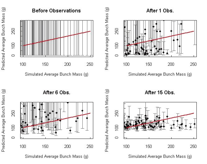
Rory Ellis et al.

such as mean and quantiles. We now turn to the                                              β0 ~ N(μβ0, τβ0)             (5)
double-sigmoidal growth model.
                                                                                            β1 ~ TN(μβ1, τ1, β0)         (6)
2.2 Double sigmoidal growth model
                                                                                            γ0 ~ TN(μγ0, τγ0, 0)         (7)
Let Yi describe the bunch mass observed at time
                                                                                            γ1 ~ TN(μγ1, τγ1, 0)         (8)
xi , i = 1...n, where n is the total number of
observations. In order to guarantee a non-                                                  τ ~ Gamma(aτ, bτ)            (9)
negative response and control for
heteroscedasticity apparent from Figures 1a, 1b,                                            Where TN(μ, τ, L) denote a normal distribution
and 1c, it is common to assume that the                                                     with mean μ and precision τ left-truncated at L.
logarithm of mass has a Gaussian distribution:                                              In order to have a priori independent parameters,
                                                                                            the model can be reparametrized in terms of Δα
                                                                                            = α1 – α0 and Δβ = β1 - β0, and the priors in Eq.
                                                                                            (4) and Eq. (6) recast as follows:
                           log(Yi) ~ N(µi, !)                          (1)

where τ is the precision or inverse variance, and                                           Δα ~ N(μΔα, τΔα, 0)          (10)
the mean expected log-mass     μi can be modelled
via the double logistic curve as follows:                                                   Δβ ~ N(μΔβ, τΔβ, 0)          (11)
                         !

                                                                                            The analysis consisted of two parts. In the first
                                                         !

                                                                                            part, for each growing season, the model was
                                              !!                   !!
 µi = f(xi, "0, "1, #0, #1, $0, $1) =                    +                    + !!   (2)
                                        !!! !!! !! !!!       !!! !!! !! !!!

where α0 and α1 describe the first and second                                               fitted to the grape bunch data available after the
asymptotes respectively, β0 and β1 are the                                                  first,
                                                                                                ( second, and up to the final (fifteenth)
inflection points, and γ 0 and γ 1 are the slope                                            observation time, assuming independent
parameters. Figure 1 illustrates the role of these                                          residuals over time, due to the destructive
parameters further. In order to analyse the model                                           measuring procedure. This was done in order to
within the Bayesian framework, we need to                                                   investigate the trade-off between an earlier
provide prior distributions for these parameters.                                           prediction and prediction accuracy, as well as to
It should be noted that we expect both slopes γ0                                            look at the growth curves fitted after one season.
and γ1 to be positive. We also do not expect the                                            In the second part, four different sets of priors
second asymptote to be less than the first; i.e., α1                                        were taken into account when analysing the
≥ α0. Note that when α1 = α0, the second term in                                            bunch mass data for the 2018/19 growing season
Equation 2 disappears and the double sigmoidal                                              in order to examine the effects of incorporating
curve collapses to a single sigmoidal curve. In                                             historical data into the modelling process. The
order to reflect these restrictions, the following                                          weakly informative priors were based on the
priors are assumed:                                                                         general expectations of the shape of the grape
                                                                                            growth curve and had high variance, and thus
α0 ~ N(μα0, τα0)                                         (3)                                small precision. The more informative prior
                                                                                            distributions were obtained by using the means
α1 ~ TN(μα1, τα1, α0)                                    (4)                                and variances of the posterior sample’s

  TABLE 1. Prior distributions used for modelling the growth of grape bunches in the 2018/19 season.
The vague prior is based on general expectations, while the parameters of the 2017, 2018, and 2017 + 2018
  priors are based on parametric approximations of the posterior distributions resulting from combining
  vague prior with the 2017 and 2018 seasons, and a combination of the two years of bunch mass data.
  Coefficient              Vague Prior                                    2017 Prior              2018 Prior            2017+2018 Prior
       !0           N(4.09,0.11)                             N(4.40,32.61)                 N(4.58, 155.24)         N(4.31, 100.77)
       "!           TN(0.69,4,0)                             TN(0.76,13.28,0)              TN(0.74,121.99,0)       TN(2.01,27.62,0)
       #0           N(200,0.02)                              N(186.89,0.93)                N(171.26,2.97)          N(181.25,1.75)
       "#           TN(49,0.11,0)                            TN(58.48,0.05,0)              TN(53.38,0.28,0)        TN(58.61,0.05,0)
        $0          TN(0.3,44.44,0)                          TN(0.09,28591.51,0)           TN(0.20,104.75,0)       TN(0.07,94918.84,0)
        $1          TN(0.3,44.44,0)                          TN(0.12,182.66,0)             TN(0.27,90.17,0)        TN(5.19*10-5,39484085,0)
        %           Gamma(4,1)                               Gamma(208.72,31.55)           Gamma(207.62,22.22)     Gamma(202.81,26.61)

 446 © 2020 International Viticulture and Enology Society - IVES                                                     OENO One 2020, 54, 2, 443-453
parametric approximation of the posterior                                     The posterior estimated mean growth curves for
distributions from the analysis of the 2017/18                                the grape bunches in the three seasons examined
bunches, the 2016/17 bunches, and by combining                                are shown in Figure 2. While all the models
the two. This was done by taking the informed                                 show a reasonable fit, there are a couple of
priors from the 2017/18 season’s bunches and                                  aspects worth noting. A clear phase II and double
informing these on the 2016/17 grape bunches.                                 sigmoid curve is apparent in the 2017/18 season
The three sets of priors are listed in Table 1.                               between days 25 and 50 (15th January to 8th
A Metropolis-Hasting sampler was written in R                                 February 2018) and to a lesser extent in 2018/19.
(Team (2015)). In each case, 105 iterations were                              This was not observed in 2016/17, for which the
run after a 2 × 10⁴ burn-in and the convergence                               resulting growth appears to be a simple sigmoid
was visually assessed.                                                        curve. Some of these differences may be
                                                                              explained by the seasonal differences in average
2.3 Simulation studies
In order to examine the effect of prior
assumptions on yield prediction, as well as to
investigate the value of information in the
context of yield prediction, 100 data sets were
simulated based on the parameters drawn from
the posterior distribution, produced after fitting
the model to the 2018/19 season’s bunch mass
data. The simulated data consisted of the mass of
15 grape bunches being measured at 15 time
points throughout the growing season. The
model described in Equations (1)-(11) was then
fitted with the four different priors described in
Table 2. The estimated posterior average bunch
mass at day 273 (the harvest day for the      ! year
2019) was then evaluated after each of the
14 measurement time points. In addition,   (12) the
                                            !

mean absolute error (MAE) was defined as !
                                                     (12)
                                       !"#
     !"# ! ! ! ! ! ! !"# ! !!"#                     (12)

Where
                                  !!                   !!
 ! !!! ! !"#! ! !"# ! !                      !
                            !!! !!! !"#!!!       !!! !!! !"#!!!

Y sim is the simulated data set and is the
simulated average bunch mass on day 273.
Similarly, the mean percentage error (MPE) was
evaluated as
                           ! !!!!!"#
               MPE = log                     (13)
                                !!"#

                      RESULTS
Individual bunch masses with the running
(geometric) mean are shown in Figure 2.
Interesting differences between the seasons are                               FIGURE 2. Individual observations and average
apparent. A clear Phase II is apparent in the                                 bunch masses (g) (solid black line) of grape
2017/18 season between days 25 and 50 (15th                                   bunches over the 2016/17, 2017/18 and 2018/19
January to 8th February 2018), which was not                                  growing seasons.
                                                                              The black dotted lines in each plot represent the posterior
observed in 2016/17. This reflects the lower                                  estimated mean growth curve for each season,
average temperature over the flowering period in                              with the surrounding grey ribbons representing the 10 %
2016/17 when compared to 2017/18, resulting in                                and 90 % estimation bounds. 2a. 2016/17 Growing season,
a longer flowering duration.                                                  2b. 2017/18 Growing season, 2c. 2018/19 Growing season
                                                                          !

                                                                      !
                                                                  !

OENO One 2020, 54, 2, 443-453                                                 © 2020 International Viticulture and Enology Society - IVES 447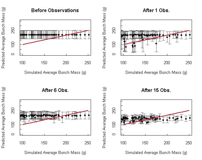
Rory Ellis et al.

FIGURE 3. The posterior mean absolute error
for the models with the vague prior,
along with the 2017, 2018, and 2017+18 priors,                     FIGURE 4. Posterior mean bunch mass curves
fitted to the grape bunch masses from the                          with bounds for the double sigmoidal model
2018/19 season after different amount of                           fitted to the data for the 2018/19 growing season
observations have been made available.                             with the vague priors, along with priors
                                                                   informing using the 2016/17 data, the 2017/18
                                                                   data, and combining them together in different
                                                                   orders (2016/17 to 2017/18 and vice versa).
temperature during flowering, and in rainfall                      The 5 % and 95 % estimation bounds are
from flowering to véraison. The average daily                      included for each set of priors.
temperature, calculated using the model
described in Trought (2005), in 2016/17 was
17.9 oC, while those in 2017/18 and 2018/19                        prediction errors for the model with vague priors
were 18.8 and 18.6 o C respectively. Lower                         are quite poor and erratic, although they do
temperatures result in a longer flowering                          improve markedly once five or more data points
duration and greater asynchronous berry                            are added (23rd January 2019).
development. The rainfall from flowering to
véraison was significantly higher in 2017/18                       Figure 4 shows the posterior mean curves and
(135 mm) than in 2016/17 and 2018/19 (49 and                       associated 95 % credible bounds, which were
41 mm respectively).                                               estimated after fitting the model to the entire
Rainfall during fruit ripening resulted in the                     2018/19 bunch mass data with the vague, the
onset of Botrytis cinerea leading to a sharp                       2017, the 2018, and the 2017 + 2018 priors
deterioration of bunch mass in 2017/18                             respectively. The results show that there is some
(Figure 2b). The data for the last observational                   apparent sensitivity to the choice of priors at
time point were therefore not included in the                      different points in the growing season. For
model, because the sharp decrease in bunch mass                    example, for the results from the incorporation of
would have affected the harvest mass estimates                     two years of priors, the estimation bounds are
produced from the Bayesian model for that                          somewhat larger than those from the other three
particular year; here, the standard double                         sets of priors. However, this switches to having
sigmoidal growth curve struggles to                                lower estimations for the bunch masses at the
accommodate the sharp rise in the middle of the                    end of the growing season.
season.
                                                                   Figure 5 compares the posterior estimates for the
The posterior estimates for the average bunch
                                                                   final bunch masses of the 2018/19 bunch mass
mass were also obtained after adding the data as
it became available consecutively to the model                     data, using each of the three informed sets of
along with the various sets of priors. The                         priors (2017, 2018, and 2017 + 2018). When
resulting mean absolute errors are shown in                        estimates are made using two years of data, they
Figure 3. The value of information is evident                      become more consistent earlier in the growing
here, along with the importance of having                          season, after about half of the data has been
informed priors, particularly at the starting of the               included in the Bayesian model. However, the
growing season. This is seen where the                             means of these estimates appear to be lower than

 448 © 2020 International Viticulture and Enology Society - IVES                            OENO One 2020, 54, 2, 443-453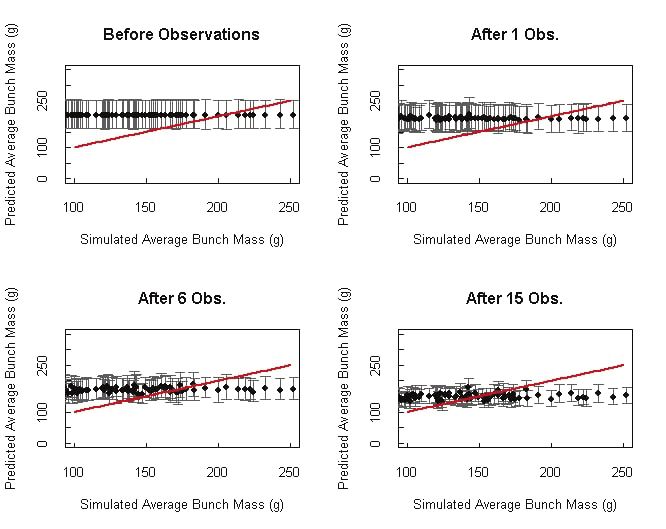
the actual final yield, as well as the estimates were evaluated a priori and after each of the
made from the other two models (2017, 2018). 14 observation time points. The results are
shown in Figures 6, 7, 8 and 9. The informative
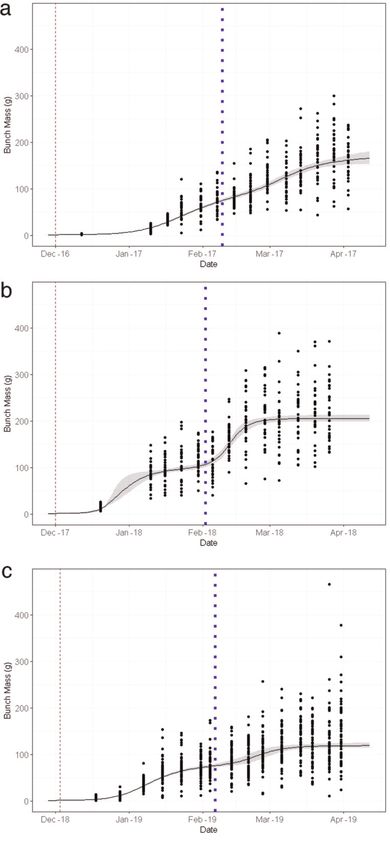
3.1 Simulation studies priors naturally have narrower credible intervals
For each of the 100 simulated datasets, the to begin with. As the season progresses and more
posterior mean bunch masses at harvest (273rd observations are collected, the intervals become
day) and the associated 95 % credible interval narrower and the predictions for the average
FIGURE 5. The predicted final bunch masses FIGURE 6. Posterior mean masses at harvest
for the 2018/19 growing season, compared (273rd day) and the associated 95 % CIs
over the 3 sets of informed priors. The 5 % for the 100 simulated datasets modelled
and 95 % estimation bounds are included for using the vague prior a priori and after the 1st
each set of priors. (18th December), 6th (31st January)
The black horizontal line represents the observed average and 15th (31st March) observation time points
final yield for the 2018/19 growing season. respectively.
FIGURE 7. Posterior mean masses at harvest FIGURE 8. Posterior mean masses at harvest
(273rd day) and the associated 95 % CIs for the (273rd day) and the associated 95 % CIs for the
100 simulated datasets modelled using the 2017 100 simulated datasets modelled using the 2018
prior a priori and after the 1st, 6th and 15th prior a priori and after the 1st, 6th and 15th
observation time points respectively. observation time points respectively.
The red line indicates equivalence. The red line indicates equivalence.
OENO One 2020, 54, 2, 443-453 © 2020 International Viticulture and Enology Society - IVES 449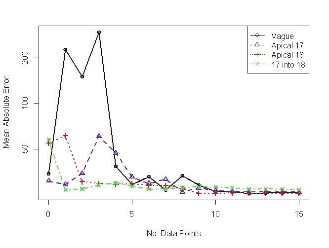
Rory Ellis et al.

                                                                   FIGURE 10. Mean absolute error for the bunch
                                                                   mass at harvest averaged over the 100 simulated
                                                                   datasets for the vague, 2017, 2018, and 2017 +
FIGURE 9. Posterior mean masses at harvest                         2018 priors respectively.
(273rd day) and the associated 95 % CIs for the
100 simulated datasets modelled using the 2017
+ 2018 prior a priori and after the 1st, 6th and
15th observation time points respectively.
The red line indicates equivalence.

bunch mass at harvest become individually
dependent on the dataset and closer to the black
line, indicating a perfect guess. It is worth noting
that the prior based on the 2017/18 growing
seasons, which was very different from the
2016/17 one, is overly conservative and is not
swayed by the data, resulting in relatively poor
predictions, even at the end of the season. The
model based on priors informed from both of
these years of data suffers even more from this,                   FIGURE 11. Mean percentage error for the mass
as the increased precision on the asymptote                        bunch at harvest averaged over the 100 simulated
parameters (α0 and Δα) keeps the means of the                      datasets for the vague, 2017, 2018, and 2017 +
posterior estimates more fixed and with tighter                    2018 priors respectively.
bounds. The model with priors informed using
two seasons of bunch mass data tended to
overestimate the bunch masses with less data,
                                                                                  DISCUSSION
and underestimate with all the data.
                                                                   Bayesian methods are capable of systematically
The resulting mean absolute error, averaged over                   incorporating prior knowledge. This feature is
the 100 datasets, is shown in Figure 10. Here, the                 especially relevant to viticulture and to grape
vague prior only starts to perform just as well as                 growth modelling, since there is substantial,
the other priors once approximately 14 of the 15                   often vineyard-specific, expert knowledge
days of data have been included, which is not                      available. The ability of the Bayesian framework
suitable given the desire to produce a model                       to seamlessly update model estimates as new
which can produce reliable estimates early in the                  data comes in is especially useful given the
growing season. However, the results shown in                      dynamic nature of the phenomenon being
Figures 10 and 11 suggest a high consistency                       modelled. Starting out with a yield estimate
throughout the growing season when using the                       based on historical data, and perhaps a general
other three priors.                                                weather forecast for the coming season, and

 450 © 2020 International Viticulture and Enology Society - IVES                            OENO One 2020, 54, 2, 443-453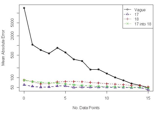
FIGURE 12. Temperature anomalies for the                FIGURE 13. Temperature anomalies for the
2016/17, 2017/18 and 2018/19 growing seasons,           2016/17, 2017/18 and 2018/19 growing seasons,
relative to the average daily temperatures              relative to the average daily temperatures
over the last 10 years.                                 over the last 10 years.

revising that estimate as new information               As a way of emphasising this, we took into
becomes available is a goal well-worth                  consideration climate information for the region
achieving.                                              in which the data was collected. Meteorological
                                                        data was sourced from the National Institute of
The model examined in this study considers the          Water and Atmospheric Research at the
bunch mass to be a function of time only. This is       Marlborough Research station 1.1 km south west
clearly an oversimplification, since plant growth       of the trial site (49 o21’51’S; 173 o 47’ 56”E).
in general, and grape growth in particular, is          Figure 12 demonstrates the temperature
known to be affected by temperature, usually            anomalies for the three growing seasons relative
expressed as growing degree days (Coombe,               to the last 10 years. The accumulated
1986). Wang and Engel (1998) introduced a               temperature experienced in the 2016/17 growing
function describing the relationship between the        season was lower than in the other seasons.
daily temperature and the daily growth date and         Above-average temperatures were noted in the
applied it to wheat growth, whereas, for                2017/18 season over the flowering period (as
example, Parker et al. (2011) and Parker (2012)         indicated by the slope of the deviation from the
extended these ideas to model phenological              long-term mean), while the other two seasons
stages of grape development. Therefore, our             were close to the long-term average over
model may be improved by replacing days with            flowering. Further heatwaves were experienced
the growth rate expressed as a function of              in both the 2017/18 and 2018/19 seasons at
growing degree days. Climate variables other            certain times in the period between flowering
                                                        and véraison (Salinger et al., 2019; Salinger et
than temperature, such as the amount of solar
                                                        al., 2020). The dates of flowering and véraison
radiation, may also influence grape growth and
                                                        were estimated using the Grapevine Flowering
development (Dokoozlian and Kliewer, 1996;              Véraison (GFV) (Parker et al., 2011). This
Bergqvist et al., 2001; Fernandes de Oliveira and       appeared to have more of a direct impact on the
Nieddu, 2016). Additional variations may arise          yield for the 2017/18 seasons, shown by the
due to characteristics of the land, such as soil and    increase in the average bunch mass
topography (Trought and Bramley, 2011;                  measurements. Figure 13 shows the accumulated
Bramley et al., 2011), as well as management            rainfall for the three growing seasons. It can be
practices. When available, this information can         seen that the 2017/18 growing season
be incorporated into the framework by                   experienced higher amounts of rainfall during
hierarchically modelling the growth curves              the course of the growing season. The 2018/19
parameters. Thus, for example, the inflection           season is typified by extended periods of no
points β0 and β1 can be construed as functions of       rainfall in the second half of the season. This
climate and spatial covariates.                         may explain the very limited amount of growth

OENO One 2020, 54, 2, 443-453                          © 2020 International Viticulture and Enology Society - IVES 451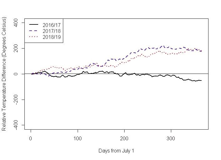
Rory Ellis et al.

in the bunch masses seen after the period of                       to the model resulted in poor results, only
véraison in this particular case.                                  becoming similar to the results seen from models
                                                                   using more informed priors once half of the
It can be seen in Figure 2a that the 6-parameter                   growing season data was incorporated into the
double sigmoidal curve was not a good fit for the                  Bayesian model. This led to the conclusion that
grape growth observed in the 2016/17 season.                       some information about the parameterisation of
Archontoulis and Miguez (2015) have reviewed                       the double sigmoidal model is influential in
a wide variety of nonlinear regression models                      producing useful results.
used in agricultural research and they have made
comparisons between various specifications of                      Acknowledgements: We would like to thank the
sigmoid functions. Of particular interest to us are                Marlborough Research Centre Trust for the use
the Richards model (Richards,1959), the                            of their vineyard.
Gompertz model (Gompertz, 1825) and the
Weibull curve (Weibull, 1951), all of which we                                     REFERENCES
intend to compare with our current
                                                                   Archontoulis S.V. and Miguez F.E., 2015. Nonlinear
implementation of the double sigmoidal model.                      regression models and applications in agricultural
It is also worth noting another more recent model                  research. Agronomy Journal 107(2), 786-798.
developed by Yin et al. (2003), which involves                     https://doi.org/10.2134/agronj2012.0506
incorporating the maximum growth rate of the
                                                                   Bergqvist J., Dokoozlian N. and Ebisuda N., 2001.
fruit to help calculate fruit mass.
                                                                   Sunlight exposure and temperature effects on berry
The current model assumed conditionally                            growth and composition of cabernet sauvignon and
independent priors and was estimated via the                       grenache in the central San Joaquin valley of
                                                                   California. American Journal of Enology and
standard Metropolis-Hasting sampler (Gelman et
                                                                   Viticulture 52(1), 1-7.
al., 2014). Taking joint prior specifications into
account will increase the flexibility of the model,                Bramley R.G., Trought M.C.T. and Praat J.-P., 2011.
allowing a wider range of expert opinion                           Vineyard variability in Marlborough, New Zealand:
formulations to be adapted, and may also                           characterising variation in vineyard performance and
                                                                   options for the implementation of precision
improve the efficiency of the algorithm.
                                                                   viticulture. Australian Journal of Grape and Wine
Finally, applying the resulting range of                           Research 17(1), 72-78. https://doi.org/10.1111/j.1755
parametrisations to a wider spatio-temporal set                    -0238.2010.00119.x
of data will improve our understanding of the                      Coombe B., 1976. The development of fleshy fruits.
modelling framework, and ultimately produce a                      Annual Review of Plant Physiology 27(1), 207-228.
better tool for early grape yield prediction.                      https://doi.org/10.1146/annurev.pp.27.060176.001231
                                                                   Coombe B., 1986. Influence of temperature on
                    CONCLUSION                                     composition and quality of grapes. Symposium on
                                                                   Grapevine Canopy and Vigor Management, XXII
In this study, we illustrated the use of a Bayesian
                                                                   IHC 206, pp. 23-36.
framework for fitting a standard double
sigmoidal growth curve to the Sauvignon blanc                      Coombe B., 1992. Research on development and
grape bunch mass data collected over the                           ripening of the grape berry. American Journal of
2016/17 2017/18 and 2018/19 growing seasons                        Enology and Viticulture 43(1), 101-110.
in Marlborough, New Zealand. We also                               Coombe B.G. and McCarthy M., 2000. Dynamics of
performed a simulation study to investigate both                   grape berry growth and physiology of ripening.
the sensitivity of the model to prior assumptions                  Australian Journal of Grape and Wine Research 6(2),
and the value of information. The latter refers to                 131-135. https://doi.org/10.1111/j.1755-0238.2000.
the role of additional consecutive observations                    tb00171.x
throughout the season in improving the accuracy                    Dokoozlian N. and Kliewer W., 1996. Influence of
of the estimation of the grape bunch mass at                       light on grape berry growth and composition varies
harvest.                                                           during fruit development. Journal of the American
                                                                   Society for Horticultural Science 121(5), 869-874.
The results from this analysis show that the                       https://doi.org/10.21273/JASHS.121.5.869
model is sensitive to prior assumptions made for                   Fernandes de Oliveira A. and Nieddu G., 2016. Vine
the parameters of the double sigmoidal model.                      growth and physiological performance of two red
From an early yield prediction perspective, the                    grape cultivars under natural and reduced UV solar
incorporation of non-informative (vague) priors                    radiation. Australian journal of grape and wine

 452 © 2020 International Viticulture and Enology Society - IVES                              OENO One 2020, 54, 2, 443-453
research 22(1), 105-114. https://doi.org/10.1111/ R.O., South P.M., Sutton P.J., Teixeira E., Thomsen
ajgw.12179 M.S. and Trought M.C.T. , 2020. Unparalleled
Fernandes T.J., Pereira A.A. and Muniz J.A., 2017. coupled ocean-atmosphere summer heatwaves in the
Double sigmoidal models describing the growth of New Zealand region: Drivers, mechanisms and
coffee berries. Ciencia Rural 47(8). https://doi.org/ impacts. Climate Change (in press). https://doi.org/
10.1590/0103-8478cr20160646 10.1007/s10584-020-02730-5
Galassi A., Cappellini P. and Miotto G., 2000. A Salinger M.J., Renwick J., Behrens E., Mullan A.B.,
descriptive model for peach fruit growth. Advances in Diamond H.J., Sirguey P., Smith R.O., Trought
Horticultural Science 19-22. M.C.T., Alexander L.V., Cullen N.J., Fitzharris B.F.,
Hepburn, C.D., Parker A.K. and Sutton P.J., 2019.
Gelman A., Carlin J. B., Stern H. S., Dunson D. B.,
The unprecedented coupled ocean-atmosphere
Vehtari A. and Rubin D. B., 2014. Bayesian Data
summer heatwave in the New Zealand region
Analysis, Third Edition (CRC Press, Taylor and
2017/18; drivers, mechanisms and impacts.
Francis: Boca Raton). https://doi.org/10.1201/b16018
Environmental Research Letters 14, 044023.
Gompertz B., 1825. Xxiv. On the nature of the https://doi.org/10.10.1088/1748-9326/ab012a.
function expressive of the law of human mortality, https://doi.org/10.1088/1748-9326/ab012a
and on a new mode of determining the value of life
contingencies. In a letter to Francis Baily, Esq. FRS Salisbury F.B. and Ross C., 2000. Fisiología de las
andc. Philosophical transactions of the Royal Society Plantas 3. Desarrollo de las plantas y fisiología
of London 115, 513-583. https://doi.org/10. ambiental (Spain, Paraninfo S.A.: Thompson
1098/rstl.1825.0026 Editores).
Mun J., 2002. Real options analysis: Tools and Tarara J.M., Blom P.E., Shafii B., Price W.J. and
techniques for valuing strategic investments and Olmstead M.A., 2009. Modeling seasonal dynamics
decisions. Volume 137 - John Wiley and Sons. of canopy and fruit growth in grapevine for
application in trellis tension monitoring. HortScience
Parker A., De Cortázar-Atauri I.G., van Leeuwen, C. 44(2), 334-340. https://doi.org/10.21273/HORTSCI
and Chuine I., 2011. General phenological model to .44.2.334
characterise the timing of flowering and veraison of
Vitis vinifera l.. Australian Journal of Grape and Trought M.C.T., 2005. Fruitset - possible
Wine Research 17(2), 206-216. https://doi.org/ implications on wine quality. Garis K. d., Dundon,C.,
10.1111/j.1755-0238.2011.00140.x Johnstone R. and Partridge S., ed. Transforming
flowers to fruit; Mildura, Australia. Australian
Parker A.K., 2012. Modelling phenology and
maturation of the grapevine Vitis vinifera L.: varietal Society of Viticulture and Oenology, 32-36.
differences and the role of leaf area to fruit mass ratio Trought M.C.T. and Bramley R.G., 2011. Vineyard
manipulations. PhD thesis, Lincoln University. variability in Marlborough, New Zealand:
Parra-Coronado A., Fischer G. and Camacho- characterising spatial and temporal changes in fruit
Tamayo J.H., 2016. Growth model of the pineapple composition and juice quality in the vineyard.
guava fruit as a function of thermal time and altitude. Australian Journal of Grape and Wine Research
Ingeniería e Investigación 36(3), 6-14. https://doi.org 17(1), 79-89. https://doi.org/10.1111/j.1755-
/10.15446/ing.investig.v36n3.52336 0238.2010.00120.x
R Core Team, 2013. A language and environment for Wang E. and Engel T., 1998. Simulation of
statistical computing. R Foundation for Statistical phenological development of wheat crops.
Computing, Vienna, Austria. URL http://www.R- Agricultural systems 58(1), 1-24. https://doi.org/
project.org/. 10.1016/S0308-521X(98)00028-6
Richards F., 1959. A flexible growth function for Weibull W., 1951. A statistical distribution function
empirical use. Journal of experimental Botany 10(2), of wide applicability. Journal of Applied Mechanics-
290-301. https://doi.org/10.1093/jxb/10.2.290 Transactions of the ASME 19(2), 293-297.
Salinger M.J., J Diamond H.J., Behrens E., Yin X., Goudriaan J., Lantinga E. A., Vos J. and
Fernandez D., Fitzharris B.B., Herold N., Spiertz H. J., 2003. A flexible sigmoid function of
Johnstone P., Kerckhoffs H., Mullan A.B., Parker determinate growth. Annals of Botany 91(3), 361-
A.K., Renwick J., Schofield, C., Siano A., Smith 371. https://doi.org/10.1093/aob/mcg029
OENO One 2020, 54, 2, 443-453 © 2020 International Viticulture and Enology Society - IVES 453You can also read